光混頻產生之連續波兆赫輻射同調性之研究

全文

(1)國立光. 電. 交工. 碩. 士. 通. 程論. 大. 研. 學. 究. 所. 文. 光混頻產生之兆輻射同調性之研究. Coherence Properties of Continuous Wave THz Radiation Generated by Photomixing on Substrates of different carrier lifetimes. 研究生：江秉其指導教授：潘犀靈. 中華民. 國九十三年. 教授. 八月.

(2) 光混頻產生之兆赫輻射同調性之研究. Coherence Properties of Continuous Wave THz Radiation Generated by Photomixing on Substrates of different carrier lifetimes 研究生：江秉其. Student: Ping-Chi Chiang 指導教. 授：潘犀靈教授. Advisor: Prof. Ci-Ling Pan. 國立交通大學光電工程研究所碩士論文 A Dissertation Submitted to Institute of Electro-Optical Engineering College of Electrical Engineering and Computer Science National Chiao Tung University In partial Fulfillment of the Requirements For the Degree of Master of Engineering In Electro-Optical Engineering July 2004 Hsinchu, Taiwan, Republic of China. 中華民. 國九十三年. 八月.

(3)

(4) 光混頻產生之連續波兆赫輻射同調性之研究研究生：江秉其. 指導老師：潘犀靈. 教授. 國立交通大學光電工程研究所. 摘要. 我們架設了一套輕便(系統大小為 50X50cm2)、便宜且輸出波長可調的連續波光源系統，來產生兆赫輻射。為了配合偵測器，我們使用 Martin-Puplett 干涉儀來量測。本論文主要利用不同載子生命期的光導天線(半絕綠砷化鎵及低溫成長砷化鎵)來產生連續波兆赫輻射，並量測其同調長度、分析。經過我們的實驗及計算推論，來得到光導天線之載子生命期和所輻射之連續波兆赫輻射的同調長度間的關連性，進而來最佳化我們連續波兆赫輻射的出輸。跟據計算，CW THz 的線寬約為 84.68MHz，而相對的同調長度為 350 公分以上，而實驗所量測同調長度為 120 公分以上，相對的線寬約為 300MHz。對於此差異，我們給予合理的解釋。. I.

(5) Coherence Properties of Continuous Wave THz Radiation Generated by Photomixing on Substrates of different carrier lifetimes Student: Ping-Chi Chiang. Advisor: Prof. Ci-Ling Pan. Institute of Electro-Optical Engineering College of Electrical Engineering and Computer Science National Chiao Tung University. Abstract We establish a small, inexpensive and movable CW THz light source to generate CW THz. In order to detect the CW THz radiation, we use Martin-Puplett interferometer with bolometer to measure it. In this thesis, we mainly use photoconductive antennas with different carrier lifetime (Semi-Insulating GaAs and Low-Temperature grown GaAs) to generate CW THz field, measure and analysis the difference of coherence length. According to our experiment and calculation, we want to find the relation between the carrier lifetime of the photoconductive antenna and the coherence length of the emitted CW THz radiation. According to our calculation , the linewidth of the CW THz radiation was about 84.68MHz, the corresponding coherence length was above 350cm. Compare with our measured coherence length of above 120cm, the corresponding linewidth was about 300MHz. we will give the reasonable answer about the difference between calculation and experiment. II.

(6) Acknowledgement 誌謝短暫的研究生涯，也是到謝幕的時候了，說起來不長不短，但這兩年中的磨練，一定會是我將來的寶藏。這些日子裡所碰到的問題實在很多，要不是有大伙的幫助，現在可能還陷在五里迷霧中，沒辦法解決。感謝潘犀靈老師這兩年的指導，指出我實驗的盲點及大方向劉子安學長實驗方面的幫助及理論方面的討論，使我在迷霧中找到一點亮光王怡超學長天線元件的製成程及為我們注入活力希望陳晉瑋學長使我有充沛的體力及銳利的口條李晁逵學長在觀念及功課方面給予幫助實驗室同伴龍進、學智、之揚、奕帆、沛霖在閒暇時聊天，困惑時互相支援學弟小冷(照仁)、小高(禎佑)、羅誠、CC(冠文)、宗翰、陳弘倫、澎湖仔(沁融)，在我苦悶、繁忙時，給予適時的幫助感謝女友瓊媛這兩年的悉心照顧、體諒，在我無助時陪伴、鼓勵我感謝我的父母、兄弟和其他家人的支持，使我生活無虞，能夠專心研究謝謝你們，僅以這本論文獻給每位幫助過我的人！！. 江秉其 2004 年 8 月于風城交大. III.

(7) Content Chinese abstract. Ⅰ. English abstract. Ⅱ. Acknowledgment. Ⅲ. Content. Ⅳ. ChapterⅠIntroduction 1.1 Background and motivation. 1. 1.2 Method of generating THz radiation. 2. 1.2.1 optical rectification. 3. 1.2.2 Photoconductive switch (current surge model). 4. 1.3 Terahertz radiation detection methods. 6. 1.3.1 Bolometer. 6. 1.3.1 Photoconductive antenna detection. 7. 1.4 Motivation and Objectives. 8. 1.5 Organization of this thesis. 9. ChapterⅡBasic theory of THz wave 2.1 THz wave generated by photoconductive. 10. antennas (current surge model) 2.2 Photomixing. 18. IV.

(8) 2.3 Coherence and Martin-puplett interferometer 2.3.1 Carrier lifetime and Coherence length 2.4Martin-Puplett polarization interferometer. 21 21 25. Chapter.Ⅲ experiment setup and result 3.1 Dual-wavelength laser diodes system. 30. 3.1.1 Laser diodes performance. 30. 3.1.2 Dual-wavelength laser diodes (LD) system. 34. 3.2 Photoconductive Antennas. 35. 3.3 Martin-Puplett Polarizing interferometer. 36. 3.3.1 Pulse THz interference result. 39. 3.3.2 CW THz interference result. 41. Chapter Ⅳ Conclusion. 45. Appendix Saturation behavior of Large-aperture Reference. 46 53. V.

(9) ChapterⅠIntroduction 1.1Background and motivation In recent years, the importance of ''terahertz light'' has increased significantly. Abbreviated THz (Existing in the region between light and radio waves), is a unit of electromagnetic (EM) wave frequency equal to one trillion hertz (1012 Hz). The terahertz is used as an indicator of the frequency of infrared (IR), visible, and ultraviolet (UV) radiation. An EM wave having a frequency of 1 THz has a wavelength of 0.3 millimeters (mm), or 300 micrometers (μm). Wireless transmissions and computer clock speeds are at frequencies far below 1 THz.. Fig.1-1 The spectrum range of electromagnetic waves [ from http://www-ece.rice.edu/]. The terahertz is not commonly used in computer and wireless technology, although it is possible that a microprocessor with a clock speed of 1 THz 1.

(10) might someday be developed. At present, the terahertz is of interest primarily to physicists and astronomers [3-8]. Research into the utilization of THz light in imaging technology and new spectroscopic technology is underway around the world [10-11]. THz light can be applied for measurements not only in the semiconductor field, but also in medical diagnoses and materials inspection. There is great potential for its application in a number of other fields as well.[3-8] Although THz frequencies are potentially very interesting, it took the development of a new technique to generate them to push them into the limelight. Traditionally, THz frequencies were generated by "heat sources" and detected with liquid-helium cooled bolometers, essentially heat detectors. In order to generate THz radiation, femto-second pulse lasers are the usual light source, such as a Ti-sapphire laser, which is expensive and large size. This laser is not available in usual laboratories and limited the THz applications. So, a compact, inexpensive and the continuous THz source is desirable. Expect the light source of CW THz, we still want to realize the relation between our THz emitters (photoconductive antennas) and the coherence length of the CW THz. Therefore, we can pick up the right emitter to generate the CW THz with longer coherence length.. 1.2 Methods of generating THz radiation During the rapid development of picosecond and femtosecond laser ，. sources in the early 1980 , there are various ways used to generate and 2.

(11) detect ultrashort-pulsed millimeter and submillimeter wave[9]. In our laboratory, we use some kinds of methods to generate and detect THz radiation, such as optical rectification、Resonant THz generation in semiconductor(such as semi-insulating GaAs and low-temperature grown GaAs) with a femtosecond pulse laser and a pair of continuous-wave (CW) laser. Followers are some methods of generation terahertz (THz) radiation.. 1.2.1Optical rectification Optical rectification is a second-order characteristic of nonlinear effect. In the electro-optic medium, the low frequency electric field is produced under intense optical illumination.Optical rectification in a non-absorbing medium is a process in which a laserpulse creates a time-dependent polarization that radiates an electric field which, in the far r. r. field, can be written according to E (t ) ∝ ∂∂t P , where the polarization P 2. 2. follows the pulse intensity envelope.. 3.

(12) Fig.1-3 Non-resonant optical rectification with a femtosecond laser pulse. It is called rectification because the rapid oscillations of the electric field of the laserpulse are "rectified" and only the envelope of the oscillations remains. In the far-field, this than changes into a pulsehape roughly sketched in the figure.Since the medium is nonabsorbing, the polarization instantanously follows the pulse envelope implying that there is practically no limit on the speed at which the polarization can be switched on and off. The polarization radiates an electrical transient which typically consists of one or one-and-a-half oscillation of the electric field and therefore has a broadband THz frequency bandwidth. Bandwidths as large as 30 THz have been obtained using this generation mechanism.. 1.2.2 Photoconductive switch (current surge model). The mechanism of generation THz radiation from the biased photoconductive switch is generally based on the current surge model. [12]In this method, if the frequency of the laser is higher than the energy needed to excite electron-hole pairs, THz generation mechanism can occur. THz electromagnetic field is radiated from a transient current which is generated on the surface of a photoconductor. Ultrashort optical pulses generate carriers instantaneously and the carriers are accelerated by the local electric field. The resultant transient current, or current surge, produces an electric field on the surface of the photoconductor and this surface field can be regarded as the source of the THz radiation. And the surface field, at the sametime, partly cancels the bias field applied to the 4.

(13) photoconductor, which is called the near-field screening effect. Fig. 1-4 shows the experimental setup for this method. Fig. 1-4 Resonant THz generation in GaAs with a femtosecond laser pulse.. We suppose to put two electrodes on the top of GaAs wafers which have different emitter structures on it, and we put a voltage across these two electrodes. When we illuminate the region between the two electrodes with a femtosecond laserpulse, the GaAs wafer suddenly becomes conducting where, before excitation, it behaved as an isolator. Under the influence of the applied electric field, a current begins to flow, which shows signs of saturation after approximately 0.5 picoseconds. Such a time-dependent current can also radiate and electrical transient, but with a higher efficiency than with non-resonant optical rectification. The frequency contents of this transient are determined by the transient behavior of the current and typically and roughly have a 3 dB bandwidth. 5.

(14) of 1 THz. This is less than what you would expect, based on the assumption that the frequency contents are determined by the laser pulse duration and that's because it isn't. It's determined by the current which can have a risetime slower that the laser pulse duration.. 1.3 Terahertz radiation detection methods. Traditionally, THz frequencies were generated by "heat sources" and detected with liquid-helium cooled bolometers, essentially heat detectors. Follower we will introduce three kinds of method to detect THz radiation, such as bolometer, photoconductive antenna detection and electro-optic sampling (e-o sampling).. 1.3.1 Bolometer. Bolometric detectors have been used for far-infrared (FIR), submillimeter- (submm) and millimeter-wave (mm) astronomy for the past 40 years. A hot electron bolometer is a device, of which the resistance responds to the change of the electron's temperature when it absorbs incident radiation. A traditional bolometer consists of a heat-sensitive detection element mounted inside a heat sink and 6.

(15) physically supported by a thermally conductive physical supporter. The most common systems are helium-cooled Si, Germanium and InSb bolometer. It can measure the power of nW grade, but it losses all the information of phase and frequency. The usual method to get the power of THz radiation is to use Martin-Puplett interferometer, we will introduce the details later.. 1.3.2 Photoconductive antenna detection. Since early 80’s, photoconductive (PC) sampling has been widely used to detect THz radiation[1]. Although its high signal to noise ratio, its speed is limited by the resonant character of the antenna structure and the finite carrier lifetime of the photocarriers[2]. Typically, the laser source is divided into two beams (pump and probe beam). When the pump beam illuminates the emitter, THz radiation is generated, then, THz and the synchronous probe beam illuminate the PC-antenna. THz radiation introduce the transient current and probe beam accelerate. 1.3.3 Electro-Optic sampling. 7.

(16) Recently, since Electro-Optic sampling has high bandwidth and is easy to implement, technique of Electro-Optic sampling became an alternative to PC detection.[9] Here, the Zinc-blende crystal was used to measure THz radiation based on the Pockels effect.[9] When we vary the temporal delay between pump and probe beam , the synchronous probe beam will probe the transient change of refractive index result from THz changing the refractive index. There is a trade-off in this method , thickness plays an important role in it, thick crystal will introduce longer interaction length but reduce the frequency response.. 1.4 Objective. Due to the advantages of CW THz system, we want to build a continuous-wave THz system including CW THz source and the detection system. Otherwise, we try to understand the relationship between carry lifetime of the photoconductive antennas and the coherence length of CW THz radiation emitted from the photoconductive antenna. First of all, we use two laser diodes to be the beating source and to illuminate the THz emitter (photoconductive antenna) to generate CW THz. In order to measure the coherence length of the CW THz, we need to use Martin-Puplett interferometer and bolometer for detection. We also want to understand the mechanism of the saturation effect of the Large-Aperture photoconductive antenna 8.

(17) 1.5 Organization of this thesis. There are four chapters in this thesis. We introduce the general conception of THz wave in Chap.1,then we give the basic theory of generation THz and the relationship between carry lifefime of the photoconductive antenna and coherence length of CW THz wave in Chap.2. At Chap.3 we give the experiment setup, results and analyses. Finally, we make some conclusions and the future work.. 9.

(18) ChapterⅡ Basic theory of THz wave In this chapter, we will introduce the basic theory of generation CW THz using photoconductive antenna as the emitter. We also introduce the coherent characteristics of CW THz radiation and the detection system (Martin-Puplett polarization interferometer).. 2.1THz wave generated by photoconductive antennas (current surge model). Photodetectors generally consist of a semiconductor material which has a bandgap energy such that it is sensitive to light in a certain wavelength range.When the photoconductive antenna is illuminated by optical source, where the photon energy is greater than the bandgap of the semiconductor (substrate of the photoconductive antenna). The photon of light can cause the generation of an electron-hole pair which under an applied electric field causes a current to flow. And the expression can be described from the current-surge model.. Initially [12], the radiating source is defined as time-varying v. parameters, including charge density ρ (x, y, z, t ) , current density J (x, y, z, t ) , r. v. electric field E (x, y, z, t ) , and magnetic flux B(x, y, z, t ) . And then, it is necessary to construct Maxwell’s equation before deducing current-surge model. Maxwell’s equation: 10.

(19) v v ∂B ∇× E = − ∂t v ρ ∇•E =. ε. v v v ∂D ∇× H = J + ∂t v ∇•B = 0. (Faraday’s Low). (2.1). (Gauss’ Low). (2.2). (Ampere’s Low). (2.3) (2.4). From (2.1) and v v B = ∇× A. (2.5). we get: v v v v ⎛ ∂A ⎞ ∂B ∂ ∇× E = − = − (∇ × A) = ∇ × ⎜⎜ − ⎟⎟ ∂t ∂t ⎝ ∂t ⎠ v ⎛ v ∂A ⎞ ⎟⎟ = 0 ⇒ ∇ × ⎜⎜ E + ∂ t ⎠ ⎝. (2.6). And then, some non-vector value, V, is induced in the equation. From (2.6), set v v ∂A − ∇V = E + ∂t v And then, ∇ × (− ∇A) = 0. (2.7) (2.8). From (2.7), v v ∂A E = −∇V − ∂t. (2.9). Next, the two inhomogeneous wave equations written in terms of A and V could also be deduced from the inhomogeneous Maxwell equations: From (2.3). 11.

(20) v v v ∂D ∇× H = J + ∂t v v ∇× B v ∂E ⇒ = J +ε ∂t µ v v B v v As H = and D = εE. (2.10). µ. Substitute (2.5) and (2.9) into (2.10), we have: v v v ⎡v ⎛v ∂E ⎞ ∂⎛ ∂A ⎞⎤ ⎟ = µ ⎢ J + ε ⎜⎜ − ∇V − ⎟⎟⎥ ∇ × (∇ × A) = µ ⎜⎜ J + ε ∂t ⎟⎠ ∂t ⎝ ∂t ⎠⎦ ⎝ ⎣ v v v v ∂2 A ⎛ ∂V ⎞ 2 ∇(∇ • A) − ∇ A = µJ − ∇⎜ µε ⎟ − µε 2 ∂t ⎠ ∂t ⎝ v 2 v v v ∂ A ∂V ⎞ ⎛ ⇒ ∇ 2 A − µε 2 = − µJ + ∇⎜ ∇ • A + µε ⎟ ∂t ⎠ ∂t ⎝. (2.11). (2.12). From (2.2), v ∇•D = ρ. v v ⎡ ⎛ ∂A ⎞⎤ ⎟⎥ = ρ ⇒ ∇ • (εE ) = −∇ • ⎢ε ⎜⎜ ∇V + ∂t ⎟⎠⎦ ⎣ ⎝ v ∂ ρ ⇒ ∇ 2V + (∇ • A) = − ∂t ε v. Set ∇ • A + εµ. ∂V =0 ∂t. (2.13). (Lorentz gauge). (2.14). So that, (2.12) becomes as v v v ∂2 A ∇ A − µε 2 = − µJ ∂t v ∂V From (2.14), ∇ • A = − µε ∂t 2. (2.15). As a result, (2.13) can be written as ∇ 2V − µε. ρ ∂ 2V = − ε ∂t 2. (2.16). Finally, the two inhomogeneous wave equations expressed in (2.15) and (2.16) are demonstrated. The two equations are used to determine a functional, time dependent form of the radiated electric field in the far 12.

(21) field. From (2.3), the continuity equation of the free carriers is obtained. r r r ∂ρ ⎛ r ∂D ⎞ ⎟ =∇• J + =0 ∇ • ∇ × H = ∇ • ⎜⎜ J + ⎟ ∂ t t ∂ ⎠ ⎝. (. ). (2.17). Actually, the current density in the bias photoconductor is strictly a transverse current (parallel to the surface of the photoconductor and perpendicular to the direction of propagation), so that r ∇• J = 0. (2.18). Equation (2.17) and (2.18) imply that the charge density dose not vary in time and not contribute to the time-dependent radiated electric field. As a result, from (2.9) the electric field is v ∂ v E rad (t ) = − A(t ) ∂t. (2.19). The solution to the wave equation (2.15) and hence for the vector v. potential A leads to the expression for the time-dependent radiated v. v. v. electric field E rad = (r , t ) at a displacement r from the center of the photoconductor: v v ⎛v r − r′ ⎞ ⎟ ⎜ J s ⎜ r ′, t − ⎟ v c 1 ∂ v ⎠da ′ ⎝ ( ) E rad r , t = − ∫ v v 2 r − r′ 4πε 0 c ∂t. (2.20). Where ε 0 is the permittivity of free space, c is the speed of light in v. vacuum, J s is the surface current in the photoconductor evaluated at the retarded time, and da ′ is the increment of surface area at a displacement v r ′ from the center of the emitter. Integration is taken over the optically. illuminated area of the photoconductor. In the far field, 13.

(22) v v v ⎛ nˆ ⋅ r ′ ⎞ r − r ′ = r ⎜1 − ⎟≈r r ⎠ ⎝. (2.21). At the same time, the gap between the electrodes of the photoconductor is assumed to be uniformly illuminated by the laser. v. Therefore, the surface current J s can be assumed to be constant at all points on the surface of the emitter. And then, the radiated electric field can be written as v v E rad (r , t ) = −. 1. (. A. 4πε 0 c 2 x 2 + y 2 + z 2. ). 1/ 2. d v ⎛ r⎞ J s ⎜t − ⎟ dt ⎝ c ⎠. (2.22). Where A is the illuminated area of the emitter. It is considered that z the radiation emitted (and detect) on axis (i.e. x=y=0), and let t → t − ⎛⎜ ⎞⎟ . ⎝c⎠. Thus, v v E rad (r , t ) ≅ −. Ad v J s (t ) 4πε 0 c 2 z dt 1. (2.23). An expression for the surface current If we want to know the radiation power of the antenna, we can use a simpler equivalent circuit of the antenna shown in figure 2-1.. Z Vb G(t). C. (a) Fig. 2-1. (b). The structure of antenna (a), and the equivalent circuit (b). 14.

(23) The equivalent circuit equation can be written as: C. dv (t ) Vb − v = − G (t )v dt Z. (2.24). where G(t) is the conductance, C is the capacitance, Z is the radiation impedance. Solve the equation (2.24), we can get: P=. P1 P2 R e η1λ1η 2 λ2 ( ) 2 2 2 hc [1 + (Ωτ ) ][1 + (ΩRC ) 2 ]. (2.25). where l1 and l2 are the wavelength of the two pump lasers, P1 and P2 are the respective pump powers, h1 and h2 are the external quantum efficiencies, W is the difference frequency, t is the photocarrier lifetime, R is the resistance of the THz load circuit, C is the photomixer capacitance, and e, h, and c are well-known physical constants. Using this CW photomixing equation, we can estimate THz power for the case of shaped pulses. Due to the high peak power of femtosecond pulses, THz intensity generated by the femtosecond pulses can easily exceed that generated by two single mode CW lasers. Another advantage is that the two frequency parts that are to be photomixed are inherently coherent, so that we can bypass the difficulty of phase-locking two ultranarrow band CW lasers. The current surge model is widely accepted as a model describing the process of THz radiation generation in biased photoconductors.[1] In this method, the surface current density Js(t) of the photoconductive emitter is related to the local applied field by Ohm’s law:. J s (t ) = σ s (t )[ Ebias + Esurf (t )] 15. (2.26).

(24) Here, σ s (t ) is the time-dependent surface conductivity, Ebias and Esurf (t ) are the static bias field applied to the emitter and the waveform of generated THz radiation field observed on the surface of the emitter, respectively. From the boundary condition of Maxwell’s equations,. Esurf (t ) is related to Js(t) as Esurf (t ) = − where. η0 1+ ε. J s (t ). (2.27). η0 is the impedance of vacuum and ε is the dielectric constant. of the emitter medium. Combine (2.26) and (2.27), an expression for. Esurf (t ) is obtained as. Esurf (t ) = −. σ s (t )η0 Ebias σ s (t )η0 + (1 + ε ). According to the relation between. (2.28). σ s (t ) and the carrier density N(t),. we can rewrite the surface field after illumination of the pump pulse is expressed as (assuming that decay of the carrier density due to recombination or trapping is slow and can be neglected in the time window of interest). Esurf (t ) = −. F Ebias F + Fsat. (2.29). where ∞. F = ∫ I (t )dt −∞. 16. (2.30).

(25) is the pump fluence and the saturation fluence ,Fsat(t), is defined as. Fsat =. hν (1 + ε ) eµη0 (1 − R ). (2.31). Where R is the reflectance of the emitter and I(t) is the pump intensity. The electric field of the focused THz pulse, E focus (t ) , has been shown to be proportional to the time derivative of the surface. By assuming the pump light to be Gaussian as. I (t ) =. F. 2. exp( δ−tt 2 ). πδt. (2.32). It can be shown that the focused field is proportional to the normalized focused field, E% focus (t ). F −t 2 exp[ 2 ] δt Fsat E% focus (t ) = F t Φ ( ) + 1]2 [ Fsat δ t. (2.33). and Φ ( x ) is defined by. Φ ( x) ≡. 1. π ∫. x. −∞. exp[− s 2 ]ds. (2.34). Finally, the expression for the normalized surface field is obtained as. Esurf (t ) / Ebias. F t Φ( ) = − Fsat δ t F t [ Φ ( ) + 1] Fsat δ t. 17. (2.35).

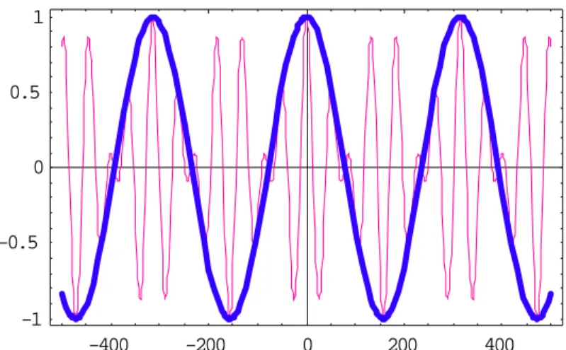
(26) 2.2 Photomixing The basic technique of generation CW THz wave is through photomixing which produces optical intensity beats at THz frequencies by mixing two single-mode lasers or mode beating within a single laser. The combination of two waves with slightly different frequencies is equivalent to a wave which envelope is modulated by the difference frequency. The intensity-modulated beam will excite the electron-hole pairs in PC antennas then accelerated by the bias voltage applied to the PC antennas. The generated THz frequency is as the same as the optical beating frequency. When two electric fields with slightly different frequencies propagate collinearly into biased PC antennas, beating signal will be radiated. Set two parallel, scalar electric fields as: E1 (t ) = E10 Cos ( w1t + φ1 ) E2 (t ) = E20 Cos ( w2 t + φ2 ). (2.36). Where E10, E20, w1, w2, f1 and f2 are the amplitudes, angular frequencies and constant phases of wave 1 and wave 2, respectively. And the total electric filed is the superposition of the two waves: E (t ) = E1 (t ) + E 2 (t ) = E1Cos ( w1t + φ1 ) + E2 Cos ( w2 t + φ 2 ). (2.37). From the simulated curves of figure 2-2, we can see that the total electric field has the waveform with a slowly various envelope and a fast carrier frequency inside.. 18.

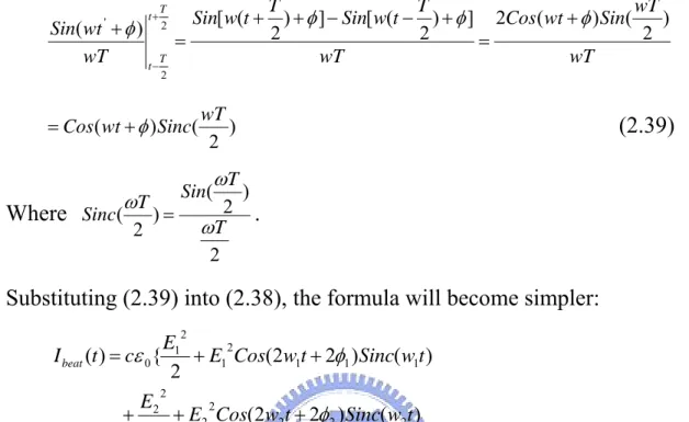
(27) 1. 0.5. 0. -0.5. -1 -400. -200. 0. 200. 400. Fig. 2-2 The simulated curves of two wave with slightly different frequencies. The thin curve is the sum of the two waves. The thick curve is the plot of the wave with frequency of (w1- w2)/2 Because the PC antenna has photocarrier lifetime about 1 ps, so it can’t response the faster frequencies. The beating intensity needs to be time averaged: t+. T. I beat (t ) = cε 0 < E 2 (t ' ) >T = cε 0 ∫ T2( E1 (t ' ) + E2 (t ' )) 2 dt ' t−. = cε. =. cε 0 T. T 2 0 T t− 2. ∫. T 2 T t− 2. ∫. t+. t+. {E1. 2. [ E1 Cos 2 ( w1t ' + φ1 ) + E 2 Cos 2 ( w2 t ' + φ2 ) + 2 E1 E2 Cos ( w1t ' + φ1 )Cos ( w2 t ' + φ2 )]dt '. 2. 2. 2. ' 1 + Cos2( w1t ' + φ1 ) 2 1 + Cos 2( w2 t + φ2 ) + E2 2 2. + E1 E2Cos[(w1t ' + φ1 ) + ( w2t ' + φ2 ))] + E1 E2 Cos[(w1t ' + φ1 ) + ( w2t ' + φ2 ))]}dt ' =. t+. T 2. t+. T 2. cε 0 Sin2( w1t + φ1 ) Sin2( w2t + φ2 ) 2 T 2 T {E1 [ + ] + E2 [ + ] T 2 2w1 2 2w2 T T t− t− '. '. 2. 2. T t+ 2. t+. T. Sin[(w1 + w2 )t ' + (φ1 + φ2 )] Sin[(w1 − w2 )t ' + (φ1 − φ2 )] 2 + E1 E2 + E1 E2 } w1 + w2 w − w T T 1 2 t− t− 2. 2. (2.38) Where c is the speed of light in vacuum, ε 0 is the permittivity of free 19.

(28) space, T is the detector response time. We know that t+. T T wT Sin[ w(t + ) + φ ] − Sin[ w(t − ) + φ ] 2Cos ( wt + φ ) Sin( ) 2 2 2 = = wT wT. T 2. Sin( wt + φ ) T wT t− '. 2. = Cos ( wt + φ ) Sinc(. Where Sinc(. ωT 2. )=. wT ) 2. Sin(. ωT. 2 ωT 2. (2.39) ). .. Substituting (2.39) into (2.38), the formula will become simpler: I beat (t ) = cε 0 {. 2. E1 2 + E1 Cos(2w1t + 2φ1 ) Sinc( w1t ) 2. 2. +. E2 2 + E2 Cos(2w2t + 2φ2 ) Sinc( w2t ) 2. (2.40). ( w + w2 )T + E1 E2Cos[(w1 + w2 )t + (φ1 + φ2 )]Sinc[ 1 ] 2 ( w − w2 )T + E1 E2Cos[(w1 − w2 )t + (φ1 − φ2 )]Sinc[ 1 ]} 2. The Sinc-function Sinc(x) plots in figure 2-3. As x values increase, y values will decrease rapidly. 1 0.8 0.6 0.4 0.2 0 -0.2 0. Fig. 2-3. 5. 10. 15. 20. The plot of Sinc-function.. 20. 25.

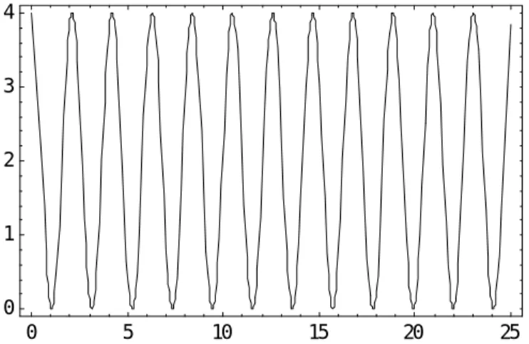
(29) When x values larger then p (3.1415), the y values are small enough to ignore it. The laser frequency is about 1015 Hz, but the fast detector response time T is just about 10-12 s. We can ignore these faster terms in equation (2.40), so the equation can be written as: cε 0 E1 cε 0 E2 ( w − w2 )T ] + + cε 0 E1 E2Cos[(w1 − w2 )t + (φ1 − φ2 )]Sinc[ 1 2 2 2 2. I beat (t ) =. 2. = I1 + I 2 + 2 I1 I 2 Cos[Ωt + φ ]. (2.41). The first two terms are the average intensities of wave 1 and wave 2, respectively. W is the difference of angular frequency between two waves. f is the phase difference of the two waves (figure 2-4). 4. 3. 2. 1. 0 0. Fig. 2-4. 5. 10. 15. 20. 25. The beating intensity with an angular frequency of W. In the simulation, we set I1 equals I2.. 2.3 Coherence and Martin-puplett interferometor. 2.3.1 Carry lifetime and Coherence length. In this thesis, we want to realize the relationship between carry 21.

(30) lifetime of photoconductive antenna’s substrate and the coherence length of CW THz wave. First, we assume that the spectrum of the light sources are Gaussian shape. Assume that the line width of the LD (source) are the. Ii (ω ) =. same,δw.. 1 e 2 δw. − ( w − wi )2. δ w2. Then, we can get the Fourier transform of Ei(ω). We only need the envelope decay term, so the Ei(t) become the last formula of equation (2.32).. 1 E1 ( w) = e δw. − ( w− w1 )2 2δ w2. ⇒ E1 (t ) = e. 1 − t (2 iw1 + tδ w2 ) 2. (2.42). E2 ( w ) = e. − ( w− w2 )2 2δ w 2. ⇒ E2 (t ) = δ we. 1 − t ( 2 iw2 +tδ w2 ) 2. Finally, follow the formula below, we can get the intensity beating signal of the CW source.. I (t ) = ( E1 (t ) + E2 (t ))( E1 (t ) + E2 (t ))∗ =e. t ( − i ( w1 + w2 )−tδ w2 ). * (e. +e. iw1t. iw2t 2. ). (2.43). and the signal in frequency domain I(ω), ∞. I ( w) = F [ I (t )] =. 1 2π. ∫. I (t )eiwt dt. −∞. we put equation (2.33) into (2.34),. 22. (2.44).

(31) I ( w) =. e. −w. 2 + ( w1− w 2 )2 2 δ w2. * (2e. w2 + 2 ( w 1− w 2 )2 4 δ w2. +e 2 *δ w. ( w + w 1− w 2 )2 4 δ w2. +e. ( w − w 1+ w 2 )2 4 δ w2. ). (2.45). From the rate equation of carrier in the substrate of the photoconductive antennas. dn(t ) I beat (t )(1 − R ) n(t ) = − τc dt hν. rate equation. (2.46). R is the reflectivity of the sample. From eq (2.23), we know that radiated THz field is proportional to the derivation of photocurrent with respect to the time. v v Erad ( r , t ) ≅ −. Ad v J (t ) 4πε 0 c 2 z dt 1. (2.23). J (t ) = n(t )q µ E. and. (2.47). Then we take the Fourier transform of the recombination of (2.46), (2.23) and (2.47). I ( w) Erad ( w ) ∝ Re{ } 1 1+ 2 2 wτ. (2.48). Finally, we find the THz field like this formula. ETHz ( w) ∝. e. − w2 + ( w 1− w 2 )2 2 δ w2. (2e. w2 + 2( w1− w 2)2 4δ w 2. ( w + w1− w 2 )2 4 δ w2. +e 1 2δ w(1 + 2 2 ) wτ. +e. ( w − w1+ w 2 )2 2 δ w2. ). We plot ETHz(w) with different carrier lifetime (1ps,10ps,100ps). 23. (2.49).

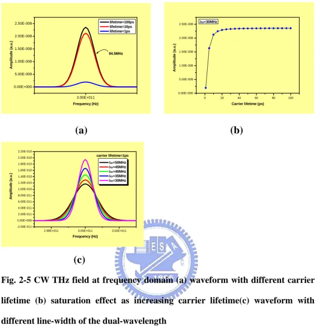
(32) lifetime=100ps lifetime=10ps lifetime=1ps. 2.50E-008. 2.50E-008. 2.00E-008. Amplitude (a.u.). Amplitude (a.u.). 2.00E-008. δω=30MHz. 1.50E-008 84.5MHz 1.00E-008. 1.50E-008. 1.00E-008. 5.00E-009 5.00E-009. 0.00E+000 0.00E+000. 3.00E+011. 0. Frequency (Hz). 20. 40. 60. 80. 100. Carrier lifetime (ps). (a). (b). 2.20E-010. carrier lifetime=1ps. 2.00E-010. δω=50MHz δω=45MHz δω=40MHz δω=35MHz δω=30MHz. 1.80E-010. Amplitude (a.u.). 1.60E-010 1.40E-010 1.20E-010 1.00E-010 8.00E-011 6.00E-011 4.00E-011 2.00E-011 0.00E+000 -2.00E-011 2.98E+011. 3.00E+011. 3.02E+011. Frequency (Hz). (c) Fig. 2-5 CW THz field at frequency domain (a) waveform with different carrier lifetime (b) saturation effect as increasing carrier lifetime(c) waveform with different line-width of the dual-wavelength. Simulation with different carrier lifetime (1, 10 and 100 picosecond), 14. the central frequency of the dual-wavelength system were 3.606*10 and 14. 3.603*10 Hz, the corresponding wavelength were about 830nm, and the line width of each laser diode was δw=30MHz. We find that the central frequency of the simulated CW THz radiation field was 0.3 THz, which was equal to the frequency difference of the dual-wavelength system. Form Fig.2-5(a), we find that the line-width of the radiation with different carrier lifetime were about 84.68MHz, the corresponding 24.

(33) coherence length was above 350cm. As we increase the carrier lifetime of the PC antenna, the calculated amplitude of CW THz radiation waveform increases, but shows the saturation effect. We plot the peak amplitude of the CW THz radiation with carrier lifetime in Fig.2-5(b). It shows much clearer that the peak amplitude of the CW THz radiation saturated when the carrier lifetime is longer than 10picosecond. It also demonstrates that the substrate of the PC antenna with carrier lifetime below 10picosecond performed as the LT-GaAs PC antenna. We changed the linewidth of the dual-wavelength system and the THz waveform was shown in Fig.2-5(c). The linewidth of the dual-wavelength system was from 30 to 50MHz, and the peak amplitude of the THz radiation was decreasing. From these mathematical analyses, we conclude that the carrier lifetime doesn’t relate to the line-width of the CW THz field, it means that carrier lifetime and the coherence length of the CW THz wave are almost independent.. 2.4 Martin-Puplett polarization interferometer The design of most interferometers used for infrared spectrometry today is based on the two-beam interferometer originally designed by Michelson in 1891. For the electromagnetic field of THz frequency range, Martin-Puplett polarization interferometer is the most usual ones, which is based on a concept originally produced by Martin and Puplett in 1969. Historically, the Martin-Puplett1 polarizing interferometer has been the spectrometer of choice at submillimetre wavelengths2 since it offers several advantages over a classical Michelson interferometer which are of 25.

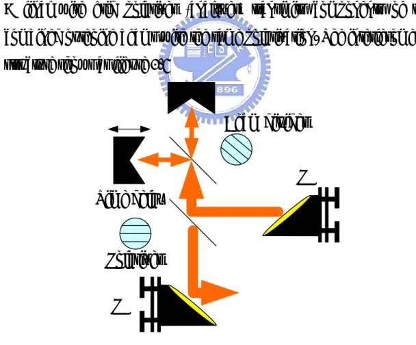
(34) particular importance in astronomical spectroscopy. For example, the modulation efficiency of a polarizing beamsplitter is both high and uniform over a wide spectral range. Martin-puplett interferometer mainly measures the Degree of Coherence function γ(τ ), the following we will describe the details. The interferometer consisted of a wire grid polarizing beam-splitter rotated 45± relative to the polarization of the incident light wave. The reflected and transmitted light waves are of equal intensity and orthogonally polarized. Retro-reflectors in each arm rotate the polarization of the incident light 180±. The orthogonal transmitted and reflected light waves are recombined at the beamsplitter. A final wire grid polarizer (analyzer) transmits components of the combined outgoing beams with the same polarization. The interferometer structure shows as figure 2-5. Beam divider. PM. Time delay. Polarizer PM. Fig. 2-6 The setup structure of Martin-puplett interferometer. 26.

(35) The total field at the detector is composed of the two beams :. v v v Ed (t ,τ ) = E (t ) + E (t − τ ). (2.50). and. v nε 0 c v E (t ) * E * (t ) 2 v nε c v I (ω ) ≡ 0 E (ω ) * E * (ω ) 2. I (t ) ≡. (2.51). from ep (2.40) and ep (2.41), we computer the intensity at the detector. v cε 0 v Ed (t ,τ ) * Ed * (t ,τ ) 2 v v cε = I (t ) + I (t − τ ) + 2 0 Re{E (t ) * E * (t − τ )} 2 I d (t ,τ ) =. (2.52). The function I(t) stands for the intensity of one of the beams arriving at the detector while the opposite path of the interferometer is blocked. For short laser pulses (sub-nanosecond), the detector automatically integrates the entire energy (per area) of the pulse since the detector cannot keep up with the detailed temporal variations of the pulse envelope. When the integration of (2.42) over time yields. ∞. ∞. ∞. ∞ v v* cε 0 ∫−∞ I d (t ,τ )dt = −∞∫ I (t )dt + −∞∫ I (t − τ )dt + 2 2 Re −∞∫ E (t ) * E (t − τ )dt. (2.53) Then, we take some mathematical tricks on eq (2.43), such as autocorrelation theorem and Parseval’s theorem. So eq (2.43) becomes. 27.

(36) ∞. ∫I. ∞. d. −∞. ∞. (t ,τ )dt = 2 ∫ I (ω )dt + 2 Re ∫ I (ω )e−iωτ dω −∞. −∞. ∞. Re ∫ I (ω )e−iωτ dω. ∞. = 2 ∫ I (ω )dω *[1 +. −∞ ∞. (2.54). ]. ∫ I (ω )dω. −∞. −∞. It is convenient to define the Degree of Coherence function. γ (τ ) , so eq. (2.44) becomes. ∞. ∫I. −∞. ∞. d. (t ,τ )dt = [2 ∫ I (ω )dt ][1 + Re γ (τ )] −∞. ∞. γ (τ ) ≡. (2.55). ∫ I (ω )e. −∞. − iωτ. dω (2.56). ∞. ∫ I (ω )dω. −∞. (2.55) describes the accumulated energy arriving to the detector after the Martin-puplett interferometer, and the entirely contained in the function. τ dependence (path delay) is. γ (τ ) .. Finally, we consider the continuous light source case (CW laser source). I ave ≡ ⟨ I (t )⟩ t =. 1 T. T 2. ∫ I (t )dt. continuous source. (2.57). −T 2. The duration T must be large enough to average over any fluctuations present in the light source. So (2.56) can be rewritten. 28.

(37) ⟨ I d (t ,τ )⟩ t = 2⟨ I (t )⟩ t [1 + Re γ (τ )]. continuous source (2.58). The degree of coherence function. γ (τ ) is responsible for. oscillations in intensity at the detector as the mirror in one of the arms is moved. The real part of. γ (τ ) is analogous to cosωτ in (2-41).. For. large delays, the oscillations tend to vanish as different frequencies individually interfere. We define the coherence time to be the function of necessary amount of delay to cause. γ (τ ) and means the. γ (τ ) to quit oscillating, so the usual. definition for the coherence time is. τc ≡. ∞. 2. ∫ γ (τ ). −∞. 2. ∞. dτ = ∫ γ (τ ) dτ. (2.59). 0. and we can find the coherence length which is the distance that light travels duration the coherence time.. lc ≡ c *τ c. (2.60). 29.

(38) Chapter.Ⅲ experiment setup and result 3.1 Dual-wavelength laser diodes system. 3.1.1 Laser diodes performance Our CW THz source are formed by two independent circular laser diodes (bluesky research PS025-00) with maximum output power 40mW and o. wavelength at 830nm. Our normal operation current is 110mA at 20 C with the output power 40mW. The L-I curve of the laser diodes are showing in Fig.3-1 and Fig.3-2. 40 35. LD1 PS025-00 Ith=31.62mA. 30. Power (mW). 25 20 15 10 5 0 0. 20. 40. 60. 80. Current (mA). Fig.3-1 L-I curve of laser diode 1 (LD1), Ith=31.62mA. 30. 100. 120.

(39) 35 30. LD2 PS025-00 ITH=32.04mA. Power (mW). 25 20 15 10 5 0 -5 0. 20. 40. 60. 80. 100. 120. Current (mA). Fig.3-2 L-I curve of laser diode 2 (LD2), Ith=32.04mA. The linewidth of LD1 and LD2 measured by Fabry-Perot interferometer are showing in Fig.3-3 and Fig.3-4, where their linewidth are 50 and 44MHz, respectively.. LD1 linewidth is about 29.3MHz FSR=2GHz. Amplitude (a.u.). 4. 2. 0. -0.015. -0.010. -0.005. 0.000. Scan time (s). Fig.3-3 Linewidth of LD1 measured by Fabry-Perot 31. 0.005. 0.010.

(40) 6. Amplitude (a.u.). LD2 linewidth is about 31.11MHz FSR=2GHz. 4. 2. 0. -0.015. -0.010. -0.005. 0.000. 0.005. 0.010. Scan time (s). Fig.3-4 Linewidth of LD2 measured by Fabry-Perot. In our experiment, we can get CW THz radiation with different central frequency by turning the wavelength of each LD. Therefore, by controlling the operation current and temperature, we can turn the wavelength difference between the two laser diodes. The accuracy of the o. LD driver and the Temperature controller are 0.1mA and 0.1 C. 836.04. LD1 ? T=19 C 0.00395nm/mA. 836.18. 836.16. LD1 I=106.6mA ? 0.0525nm/ C. Wavelength (nm). Wavelength (nm). 836.02. 836.00. 835.98. 836.14. 836.12. 836.10. 836.08 835.96. 836.06 85. 90. 95. 100. 105. 110. 19.0. 19.5. ?. 20.0. 20.5. 21.0. T( C). Current (mA). (a) Temperature control. (b) Current control. Fig.3-5 LD1 wavelength shift (a) controlling current at 19 32. o. C.

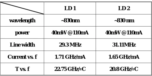
(41) (b) controlling the temperature at operation current=106.6mA. 835.48. LD2 ? T=19 C 0.00381nm/mA. 835.46. 835.58. LD2 I=108.6mA ? 0.048nm/ C. Wavelength (nm). Wavelength (nm). 835.56 835.44. 835.42. 835.40. 835.54. 835.52. 835.50. 835.38. 835.48. 85. 90. 95. 100. 105. 110. 19.0. 19.5. ?. 20.0. 20.5. 21.0. T( C). Current (mA). (a) Temperature control. (b) Current control. Fig.3-6 LD2 wavelength shift (a) controlling current at 19. o. C. (b) controlling the temperature at operation current=108.6mA. Form Fig.3-5 and Fig.3-6, the wavelength shift caused by changing current are 0.00395nm/mA and 0.00381 nm/mA, respectively; the shift o. o. caused by shifting temperature are 0.0525nm/ C and 0.048/ C , respectively. Table 3-1 show the summary of the two LD. 33.

(42) LD 1. LD 2. wavelength. ~830nm. ~830 nm. power. 40mW @110mA. 40mW @110mA. Line width. 29.3 MHz. 31.11MHz. Current vs. f. 1.71 GHz/mA. 1.65 GHz/mA. T vs. f. 22.75 GHz/∞C. 20.8 GHz/∞C. Table 3-1 The characteristics of the two laser diodes. 3.1.2 Dual-wavelength laser diodes (LD) system Our dual-wavelength light source system is presented in Fig.3-7. It is composed by two frequency-independent laser diodes (bluesky research PS025-00) and some proper optics. The polarization of the LD is S polarization. The 40X objective lens are used to focus the spot size of the two LD, when light passed through the isolator, the polarization of the incident light will be rotated to 45 °C to prevent the optical feedback from other optics, when the light passed through the half-wave plate, the polarization will be changed from linear polarization to elliptical polarization.. 34.

(43) λ /2. PBS. LD1. isolator. PBS. λ /2. λ /2 isolator. LD2. (a). (b). Fig.3-7 Dual-wavelength system (a) diagram of the system (b) the actual system. 3.2 Photoconductive Antennas Due to our purpose, we need to have two kinds of antennas (Low-Temperature grown GaAs and Semi-Insulating GaAs) with different carrier lifetime and the same structure. Carrier lifetime of Low-Temperature grown GaAs and Semi-Insulating GaAs are few and hundreds of pico-seconds and the structure are bow-tie structure.. θ. 1mm / θ = 90o. (a). (b). 35.

(44) Intensity (a.u.). 1. 0.1 0.0. 0.2. 0.4. 0.6. 0.8. Frequency (THz). (c). (d). Fig.3-8 (a) the actual structure of the antenna (b) the diagram of the antennas (c) frequency response of SI GaAs antenna (d) frequency response of SI GaAs antenna. 3.3 Martin-Puplett Polarizing interferometer In order to get the power spectrum of the CW THz radiation, we set up a Martin-Puplett interferometer, the whole setup is in Fig.3-9 (a). When the CW light source illuminates the photoconductive antenna, we use the method showing in Fig.3-9, the radiation from the bow-tie antennas is linearly polarized in the bow-tie direction, and its polarization is oriented so as to pass through the wire-grid polarizers at the input port of a Martin-Puplett interferometer. The interferometer consisted of two °. wire-grid polarizers with 45 C polarization with respect to each other in order to divide the THz radiation into two parts, one of which was reflected by a fixed mirror and the other is reflected by a scanning mirror.. 36.

(45) The interferometer signal at the output port is measured with a Silicon hot-electron bolometer cooled to 4.2 K. The laser beam is chopped at 187Hz and the modulated signal voltage from the bolometer is detected with a lock-in amplifier. Beam divider. Antenna Si-lens. Time delay PM. Polarizer PM. Bolometer. Fig.3-8 (a) diagram of Martin-Puplett interferometer. 37. Lock-in Amplifier.

(46) Fig.3-8(b)the actual setup of the Martin-Puplett interferometer. BS. 10 X Objective lens. Screen. Antenna. Fig.3-9 the method to check laser beam illuminating the gap of antenna. Before using the CW laser to excite the CW THz radiation, we use the femto-second pulse laser illuminating the antenna to calibrate the Martin-Puplett interferometer and the contact between Si-lens and the photoconductive antenna. The contact plays an important role in this 38.

(47) experiment. Next, we show the power spectrums of three kinds of antennas (LT-GaAs、SI- GaAs bow-tie and SI- GaAs lateral offset dipole) illuminated by femo-second and measured by bolometer.. 3.3.1 Pulse THz interference result. According to our purpose, we need to check the contact between antenna and si-lens. We use femto-second pulse laser optimize the condition. 0.006 0.004. Amplitude (a.u.). 0.002 0.000 -0.002 -0.004 -0.006 -0.008 -0.010 -0.012. SI-GaAs bow-tie step 0.01mm point 200 timeconst 300ms. -0.014 0. 2. 4. 6. 8. 10. 12. time delay (ps). (a) Power spectrum of SI GaAs. 39. 14.

(48) Frequency (Hz). Angle(deg). 0. 2. 4. 6. 8. 4. 6. 8. 0 -2000 -4000 -6000 -8000. 1E-3. 0.293THz. Amplitude. 1E-4. 1E-5. 1E-6 0. 2. Frequency (Hz). (b) FFT of (a) Fig.3-10 material :SI GaAs, structure :bow-tie(a)power spectrum (b)FFT of (a) For LT GaAs bow-tie photoconductive antenna, we get the small signal. 0.00005. Amplitude (a.u.). 0.00000. -0.00005. -0.00010. -0.00015. LT GaAs bow-tie step 0.01mm point 200 timeconst 300ms. -0.00020. -0.00025 0. 2. 4. 6. 8. 10. 12. Timedelay (ps). (a) Power spectrum of LT GaAs. 40. 14.

(49) Frequency (Hz) Angle(deg). 0. 2. 4. 6. 8. 4. 6. 8. 0 -2000 -4000 -6000. 1E-5. Amplitude. 0.35THz. 1E-6. 1E-7. 0. 2. Frequency (THz). (b) Fig.3-11 material : LT GaAs, structure :bow-tie(a)power spectrum (b)FFT of (a). For SI GaAs photoconductive antennas, the dark current is about ten μ m and we apply bias at 18V, and the photo-current is about 1.4mA. The dark current on LT-GaAs is about 0.5μA, bias at 30V, the photo-current arrives 0.3mA. The pulse interference signal of SI GaAs is over a hundred times than that of LT GaAs, this may results from the different prescriptions of the ohmic contact of the antennas. From Fig.3-10 and 3-11, we can find that the THz radiation signal of SI-GaAs is larger than that of LT-GaAS. This result can also be get from Fig.2-5. Emitter with longer carrier lifetime will have larger amplitude of its signal.. 3.3.2 CW THz interference result We can change the wavelength difference by tuning the temperature and operation current. The wavelength difference 0.66nm is chosen, corresponding to 0.258THz. 41.

(50) 0. δλ=0.66nm. power (dBm). -10. -20. -30. -40. -50. 828. 830. 832. 834. 836. 838. 840. wavelength (nm). Fig.3-12 The spectrum of the LD. Amplitude (a.u.). 0.00012. 0.00008. 0.00004. 0.00000. -0.00004. -0.00008 0. 50. 100. 150. Time delay (ps). (a). 42. 200. 250.

(51) Frequency (Hz) 0. 2. Angle(deg). 500 0 -500 -1000 0.00004. 0.2587THz. Amplitude. 0.00003. 0.00002. 0.00001. 0.00000 0. 2. Frequency (THz). (b) Fig.3-13(a) for SI GaAs photoconductive antenna. According to Kuo’s thesis, we can realize that the coherence length of the CW THz radiation was about more than 100cm, the corresponding line-width of the CW THz radiation was about 250MHz.The total length of the delay stage is 30cm. We scan about 20cm, corresponding to total delay 40cm. We divide the measurement into several parts for cooling the antenna. The CW THz interferometer is shown in Fig.3-13(a) for SI GaAs photoconductive antenna. The contact of the antenna and the Si-lens plays an important role for this measurement, and the tilt of the Si-lens also affects our measurement. From the measurement result and the comparison with our calculation, the coherence length of the CW THz radiation does not relate to the carrier lifetime of the substrate of the PC antenna. SI-GaAs photoconductive antenna has carrier lifetime of tens of picoseconds, 43.

(52) however, it can perform as well as the LT-GaAs PC antenna, and its signal is larger than that of LT-GaAs PC antenna.. 44.

(53) Chapter Ⅳ Conclusion We have built the CW THz source and the CW THz detection system – Martin-Puplett interferometer. Using the dual-wavelength system as the CW THz source. According to our mathematical calculation in ChapterⅡand our experiment result, we make some statements that the coherence length of the CW THz generated by photoconductive antennas doesn’t have apparent relation with the carrier lifetime of the emitters (photoconductive antennas). And as we increase the carrier lifetime of the PC antenna, the calculated amplitude of CW THz radiation waveform increases, but shows the saturation effect shown in Fig.2-5. We plot the peak amplitude of the CW THz radiation with carrier lifetime in Fig.2-5(b). It shows much clearer that the peak amplitude of the CW THz radiation saturated when the carrier lifetime is longer than 10picosecond. It also demonstrates that the substrate of the PC antenna with carrier lifetime below 10picosecond performed as the LT-GaAs PC antenna. We changed the linewidth of the dual-wavelength system and the THz waveform was shown in Fig.2-5(c). The linewidth of the dual-wavelength system was from 30 to 50MHz, and the peak amplitude of the THz radiation was decreasing.. 45.

(54) Appendix Saturation behavior of Large-aperture In order to understand the saturation behavior of intense THz radiation emitted by a large-aperture photoconductive antenna was studied by observing the waveforms to the generated THz pulse using the electro-optic sampling method. We use two kinds of different material to probe into the saturation effect. The samples are GaAs:As+ and SI GaAs, and it’s gap are 5μm. In this experiment, we generated intense THz radiation from a large-aperture GaAs photoconductive antenna and observed the waveforms of the field of focused THz radiation using the EO sampling method. BS. Mirror. Delay scan. Polarizer. Chopper. PM3. PM4. Attenuator. Antenna. Pellicle BS. Mirror ZnTe PM1. PM2. QWP Wollaston. Prism Detector. PM1~4: Parabolic Mirror. Fig.A-1 Electro-optic sampling system structure. 46.

(55) 1. Amplitude(a.u.). Amplitude(a.u.). Pump Fluence 2 2 µJ/cm 2 9.2µJ/cm 2 18 µJ/cm 2 30 µJ/cm 2 44 µJ/cm 2 58 µJ/cm. 0. 0. -1. 0. 20. Pump Fluence 2 2 µJ/cm 2 9.2µJ/cm 2 18 µJ/cm 2 30 µJ/cm 2 44 µJ/cm 2 58 µJ/cm. 1. 0. 5. 0.01. 15. 20. 0.01. 1E-3. Amplitude (A.U.). Amplitude(A.U.). 10. Time delay(ps). Time delay(ps). 1E-4. 1E-3. 1E-4. 1E-5. 0.0. 0.5. 1.0. 1.5. 2.0. 2.5. 0.0. Frequency (THz). 0.5. 1.0. 1.5. 2.0. 2.5. Frequency (THz). (a) GaAs:As+. (b) SI GaAs. Fig.A-2 (a) GaAs:As+ and (b) SI GaAs are the THz waveform measured by EO sampling and it’s FFT. Fig.A-2shows the typical waveform of focused THz radiation measured by the EO sampling, obtained at several pump fluence. The FFT of the THz waveform also shows in this Figure, the spectrum extends from dc component to above 2.5THz. we can find a dip around 1.7THz is due to water vapor absorption.. By increasing the pump pulse fluence, saturation of the peak THz field, shift of the peak appearance time and narrowing of the THz pulse were observed.. 47.

(56) 52µJ/cm linear fit. 400. Peak THz Amplitude(a.u.). Peak THz Amplitude(a.u.). 450. 2. 350 300 250 200 150 100 50. 600 500 450 400 350 300 250 200 150 100 50 0. 50. 100. 150. 200. 250. 2. 58µJ/cm linear fit. 550. 300. 0. 50 100 150 200 250 300 350 400 450 500 550. Bias Field(kV/cm). Bias Field(kV/cm). (a) GaAs:As+. (b) SI GaAs. Fig.A-3 (a) and (b) are bias field dependence of peak THz field. Fig.A-3 shows the peak field of THz pulses is plotted as a function of the bias field and the peak field is proportional to the bias field within the range of bias field.. 2.0. Amplitude(a.u.). 1.6 1.4 1.2 1.0 0.8 0.6 0.4 0.2. 2.0 Pump Fluence 2 2 µJ/cm 2 9.2µJ/cm 2 18 µJ/cm 2 30 µJ/cm 2 44 µJ/cm 2 58 µJ/cm. 1.8. Amplitude(a.u.). Pump Fluence 2 2 µJ/cm 2 9.2µJ/cm 2 18 µJ/cm 2 30 µJ/cm 2 44 µJ/cm 2 58 µJ/cm. 1.8. 0.0. 1.6 1.4 1.2 1.0 0.8 0.6 0.4 0.2 0.0. -0.2 -0.7 0.0 0.7 1.4 2.1 2.8 3.5 4.2 4.9 5.6 6.3 7.0. -0.2 -1. Time(ps). 0. 1. 2. 3. 4. 5. 6. 7. Time(ps). (a) GaAs:As+. (b) SI GaAs. Fig.A-4 (a) and (b) are waveforms of THz radiation around the peak at several pump fluence values. 48.

(57) Peak THz Amplitude(µV). 350 300 250 200 150 100 +. As -GaAs. 50. SI-GaAs. 0 -50 -20. 0. 20. 40. 60. 80. 100 120 140 160 180 2. Laser Fluence(µJ/cm ). Fig.A-5 Pump fluence dependence of peak THz amplitude at bias field equaling 0.6KV/cm. From Fig.A-5 The peak THz field showed clear saturation behavior as a function of pump fluence of GaAs:As+ and SI GaAs. The thermal carrier scattering effect on GaAs:As+ is less than that on SI-GaAs.. 0.72. 0.69 0.68. 0.75 0.10. 0.74 0.05. 0.73 0.72. 0.00. Peak Shift(ps). 0.05. Pulse Width(ps). 0.70. 0.15. Peak Shift(ps). Pulse Width(ps). 0.76 0.10. 0.71. 0.00. 0.67. 0.71 0. 10. 20. 30. 40. 50. 60. 0. 10. 20. 30. 40. 50. 60. 2. Pump Fluence(µJ/cm ). 2. Pump Fluence(µJ/cm ). (a) GaAs:As+. (b) SI GaAs. Fig.A-6Experimentally observed pulse width and shift of peak appearance time are plotted as a function of pump fluence for (a) GaAs:As+ and (b)SI GaAs.. 49.

(58) From Fig.A-6, the shift of peak appearance time shows almost linear dependence on the pump fluence. On the other hand, pulse width shows almost a saturation behavior before 50μJ/cm2.. After 50μJ/cm2, the. pulse width increase with the pump fluence. From (2.35)and (2.33) in chapterⅡ, we can make some simulation of the saturation of the large-aperture photoconductive antennas. We can choose the normalized pump fluence, F/Fsat, to find the pump fluence dependence of the normalized surface field.. S u rf a c e f i el d. 0.8 0.6 0.4 0.2 0 -4. -2 0 2 t Normalized time A E δt. 4. Fig.A-7 Simulated normalized surface field at three values of pump fluence. 50.

(59) peak shift. THz field. 1 0.8 0.6 0.4 0.2 0 -4. -2 0 2 t Normalized time A E δt. 4. Fig.A-8 Simulated waveforms of normalized focused THz radiation at three values of normal pump fluence. It is clearly seen from Fig.A-8 that the value of the peak THz field saturates as a function of the pump fluence, and the peak shift temporally to the negative direction, and the pulse width is narrowed by increasing the pump fluence. 1.6 0.5. 1.4. 0.3 0.2. Peak shift/δt. Pulse width/δt. 0.4. 0.1. 1.2 0.0. 2. 4. 6. 8. 10. Normalized pump fluence,F/Fsat. Fig.A-9 Stimulated Pump fluence dependence of the Pulse width and shift of the peak position of the focused THz field 51.

(60) Fig.A-9 shows the theoretical result, we can find that there is no saturation effect in the pulse width narrowing, and the peak shift shows almost linear toward normalized pump fluence.. 52.

(61) Reference [1]. Q. Wu and X.-C. Zhang, IEEE J. Sel. Top. Quantum Electron. 2,693,1996.. [2] S.-G. Park, M. R. Melloch and A. M. Weiner, “Comparison of terahertz waveforms measured by electro-optic and photoconductive sampling,” Appl. Phys. Lett., vol.73, no.22, pp.3184-3186,1998. [3]. Bradley Ferguson, and Xi-Cheng Zhang, “Materials for terahertz science and technology,” Nature, Vol. 1, pp. 26-33, 2002.. [4]. M Usami, T Iwamoto, R Fukasawa et al, “Development of a THz spectroscopic imaging system,” Phys. Med. Biol., Vol. 47, pp. 3749–3753, 2002. [5] P Y Han and X-C Zhang, “Free-space coherent broadband terahertz time-domain spectroscopy” Meas. Sci. Technol., Vol. 12, pp. 1747-1756, 2001 [6]. Masahiko Tani1, Michael Herrmann and Kiyomi Sakai, “Generation and detection of terahertz pulsed radiation with photoconductive antennas and its application to imaging,” Meas. Sci. Technol., Vol. 13, pp. 1739-1745, 2002. [7]. Daniel M. Mittleman, Rune H. Jacobsen, and Martin C. Nuss, “T-Ray Imaging,” IEEE J. Selected Topics in Quantum Electronics, Vol. 2, No. 3, pp. 679-692, 1996. [8]. AG Davies, EH Linfield and M B Johnston, “The development of terahertz sources and their applications,” Phys. Med. Biol., Vol. 47, pp. 3679–3689, 2002 53.

(62) [9] Sang-Gyu Park, M. R. Melloch, and A. M. Weiner, “Comparison photoconductive sampling,” Appl. Phys. Lett., Vol.73,pp. 3184-3186,1998. [10] D. Grischkowsky, S. Keiding, M. van Exter, and Ch. Fattinger, J. Opt.Soc. Am. B, Vol. 7, pp,2006,1990. [11] I. Brener, D. Dykaar, A. Frommer, L. N. Pfeiffer, J. Lopata, J. Wynn, K. West, and M. C. Nuss, Opt. Lett. Vol. 21, pp. 1924, 1996. [12] Justin T. Darrow, Xi-Cheng, David H. Austion, Fellow, IEEE, and Jeffrey. D.. Morse,. “Saturation. properties. of. large-aperture. photoconducting antennas,” IEEE J. Quantum electron., Vol.28, no.6, pp.1607-1616,1992. [13] P. K. Benicewicz, J. P. Roberts, and A. J. Taylor, “Scaling of terahertz radiation from large-aperture biased photoconductors, ” J. Opt. Soc. Am. B, Vol.11, no. 12, pp. 2533-2546,1994. [14] Rü deger Kő hler, Alessandro Tredicucci, Fabio Beltram,Harvey E. Beere, Edmund H. Linfield, A. Giles Davies,David A. Ritchie, Rita C. Iotti & Fausto Rossi, “Terahertz semiconductor heterostructure laser,” Nature, Vol. 417, pp. 156-159, 2002. [15] Ping GU, Masahiko Tani, Masaharu Hyodo, Kiyomi Sakai, and Takehiro Hidaka, “Generation of cw-Terahertz Radiation Using a Two-Longitudinal-Mode Laser Diode,” Jpn. J. Appl. Phys., Vol. 37, Part2, no. 8B, pp. L976-L978, 1998. [16]. Masahiko. Tani,. Shuji. Matsuura,. Kiyomi. Sakai. et. al,. “Multiple-Frequency Generation of Sub-Terahertz Radiation by Multimode LD Excitation of Photoconductive Antenna,” IEEE Microwave and Guided Wave Lett., Vol. 7, pp. 282-284, 1997. [17]. D. H. Martin, and E. Puplett, “Polarised interferometric 54.

(63) spectrometry for the millimetre and submilimetre spectrum,” Infrared Physics, Vol. 10, pp. 105-109, 1969. [18]. Masahiko Tani, Shuji Matsuura, Kiyomi Sakai, and Shin-ichi Nakashima, “Emission characteristics of photoconductive antennas based on low-temperature-grown GaAs and semi-insulating GaAs,” Appl Opt, Vol. 36, pp. 7853-7859, 1997.. [19]. Dongfeng Liu and Jiayin Qin, “Carrier dynamics of terahertz emission from low-temperature-grown GaAs, ”Appl Opt, Vol. 42, no. 18, pp. 3678-3683,2003.. [20] Toshiaki Hattor, Keiji Tukamoto, and Hiroki Nakatsuka, “Time-Resolved Study of Intense Terahertz Pulses Generated by a Large-Aperture Photoconductive Antenna, ” Jpn. J. Appl. Phys., Vol. 40, pp. 4907-4912,2001. [21] Ajay Nahata, David H. Auston, and Tony F. Heinz, “Coherent detection of freely propagating terahertz radiation by electro-optic sampling, ” Appl. Phys. Lett., Vol. 68, pp. 150-153,1995. [22] Ajay Nahata, James T. Yardley, and Tony F. Heinz, “Free-space electro-optic detection of continuous-wave terahertz radiation,” Appl. Phys. Lett., Vol. 75, no.17, pp. 2524-2526,1999. [23]. Sang-Gyu Park, Michael R. Melloch, and Andrew M. Weiner, “Analysis of Terahertz Waveforms Measured by Photoconductive and Electrooptic Sampling,” IEEE J. Quantum Electronics, Vol. 35, no. 5, pp.810-819, 1999.. [24]. Shunsuke. Kono,. Masahiko. Tani,. and. Kiyomi. Sakai,. “Ultrabroadband photoconductive detection: Comparison with free-space electro-optic sampling,” Appl. Phys. Lett., Vol. 79, no. 7, pp. 898-900, 2001. [25]. Paul C. M. Planken, Han-Kwang , Huib J. Bakker et al, “Measurement and calculation of the orientation dependence of the 55.

(64) terahertz pulse detection in ZnTe,” J. Opt. Soc. Am. B, Vol. 18, no.3, pp.313-317, 2001. [26] K. A. McIntosh, E. R. Brown, K. B. Nichols et al, “Terahertz photomixing with diode lasers in low-temperature-grown GaAs,” Appl. Phys. Lett., Vol. 67, no. 26, pp. 3844-3846, 1995.. 56.

(65)