國立交通大學
電子工程學系 電子研究所
碩士論文
在時變多路徑通道之低複雜度載波間互擾
效應消除於正交分頻多工系統
A Low-Complexity ICI Cancellation Scheme For
OFDM In Time-Varying Multipath Channel
研究生:劉仲康
指導教授:桑梓賢 教授
在時變多路徑通道之低複雜度載波間互擾
效應消除於正交分頻多工系統
A Low-Complexity ICI Cancellation Scheme For OFDM
In Time-Varying Multipath Channel
研 究 生:劉仲康 Student:Chung-Kang Liu
指導教授:桑梓賢 Advisor:Tzu-Hsien Sang
國 立 交 通 大 學
電子工程學系 電子研究所
碩 士 論 文
A ThesisSubmitted to Department of Electronics Engineering & Institute of Electronics College of Electrical Engineering and Computer Engineering
National Chiao Tung University in partial Fulfillment of the Requirements
for the Degree of Master
in
Electronics Engineering January 2007
Hsinchu, Taiwan, Republic of China
在時變多路徑通道之低複雜度載波間互擾效應消除
於正交分頻多工系統
研究生: 劉仲康
指導教授: 桑梓賢 博士
國立交通大學
電子工程學系 電子研究所碩士班
摘要
本篇論文應用在正交分頻多工(OFDM)系統於時變頻率選擇衰變通
道. 隨著符號長度的增加,OFDM 可抵抗對於多重路徑干擾的效應。然而在
行動通訊的應用上,時變通道破壞了子載波間的正交性,造成載波間的互
相干擾(ICI)因而降低系統效能。在本篇論文中,利用線性模型去近似時
變通道。基於這個假設,我們解出線性的通道參數進而重建通道矩陣,目
的去消除載波間的互相干擾。模擬結果顯示所提出的方法可有效抑制因時
變通道所造成的 ICI 效應以及降低錯誤率在高雜訊比仍高居不下的現象。
A Low-Complexity ICI Cancellation Scheme For OFDM In
Time-Varying Multipath Channel
研 究 生:劉仲康 student:Chung-Kang Liu
指導教授:桑梓賢 Advisors:Tzu-Hsien Sang
Department of Electronics Engineering & Institute of Electronics
National Chiao Tung University
ABSTRACT
This thesis considers an orthogonal frequency division multiplexing (OFDM)
system over frequency selective time-varying fading channels. As the symbol
duration increases, OFDM is robust to channel multipath dispersion. However,
for mobile applications, channel variations within an OFDM block period
destroy the orthogonality between subcarriers; the effect, known as Intercarrier
Interference (ICI), will degrade the system performance. In this thesis, a linear
model is assumed for the channel variation because of its simplicity. Based on
the assumption, the proposed method solves the linear channel parameters of
each path and creates a channel matrix which can be used for ICI cancellation.
The simulation results show that the proposed method can effectively suppress
the ICI effects induced by the time variant channels and reduce the error floor of
bit error rate (BER).
誌謝
兩年半的研究所生活也到了尾聲, 首先感謝我的指導教授桑梓賢博士,
對於我的研究方向給予很多的建議及指導, 讓我可以順利完成這篇論文. 同
時也感謝欣徳學長在這兩年之中的協助, 一些經驗的傳承給予我很大的收
穫.當然也要感謝實驗室的同學們,在有問題時可以與你們討論找出自己的盲
點, 很高興認識你.
最後,感謝我的父母,無怨無悔的給予我生活上的精神上的支持,以及我
女朋友謝小明在我在苦惱的時候也在旁鼓勵我,總之感謝各位.
Contents
中文摘要………...I
ABSTRACT………...II
誌謝……..……….…..III
CONTENT……….…..Ⅳ
LIST OF TABLES………...………Ⅳ
LIST OF FIGURES..………...…… V
Chapter1 Introduction ... 1 1.1 Motivation ... 1 1.2 Literature survey ... 1 1.3 Thesis organization... 2Chapter 2 OFDM Communication Systems in Wireless Channels... 3
2.1 System model ... 3
2.2 Inter-carrier interference in OFDM systems induced by Doppler effect... 5
Chapter 3 ICI Mitigation in Doppler Spread Channel ... 8
3.1 Pilot-based channel estimation... 8
3.2 The proposed method... 10
3.3 Computation complexity analysis ... 15
Chapter4 Simulations and Discussions... 17
4.1 Simulation result... 17
4.2 Conclusion ... 24
LIST OF TABLES
Table 1 Computational complexity analysis ... 16
Table 2 Simulation parameters... 17
Table 3 Overhead, complexity and performance of the various schemes ... 23
LIST OF FIGURES
Fig. 1 System model... 3Fig. 2 Normalized symbol energy distribution... 6
Fig. 3 Comb-type pilot arrangement ... 8
Fig. 4 Block diagram of the estimation of the channel matrix ... 12
Fig. 5 Transmitted data format 1 ... 12
Fig. 6 Transmitted data format 2... 13
Fig. 7 Banded channel matrix with color region corresponding to ICI concentration .... 14
Fig. 8 Block diagram of the proposed ICI-reduction method ... 15
Fig. 9 Generation of the tap weight processes... 18
Fig. 10 BER performance of ICI reduction algorithm with f Td s =0.04... 19
Fig. 11 The comparison of partial ICI reduction method ... 19
Fig. 12 BER performance of ICI reduction algorithm with f Td s =0.1... 20
Fig. 13 BER performance of ICI reduction algorithm with f Td s =0.2... 21
Fig. 14 BER performance of proposed method with f Td s =0.04 and various CFO ... 21
Fig. 15 BER performance of proposed method with f Td s =0.04 and various timing offset ... 22
Chapter1
Introduction
1.1 Motivation
OFDM is a widely used and considered a promising technique for high speed data transmission in digital audio broadcasting (DAB) systems, digital video broadcasting (DVB)systems, and for wireless broadband access standard such as IEEE Std. 802.16 (WiMAX). OFDM is robust to channel multipath dispersion and results in a decrease in the complexity of equalizers for high delay spread. However, using conventional channel equalization without ICI compensation results in an error floor in mobile OFDM systems [1]. Channel estimation schemes for mobile OFDM systems, in contrast to stationary channel where solely the frequency selectivity has to be estimated, also have to estimate the time variation of the mobile channel. In the thesis, a new ICI reduction method is proposed, which reduces the error floor caused by the channel variation.
1.2 Literature survey
To mitigate the ICI caused by channel variation, many approaches have been proposed, e.g., polynomial cancellation coding [2], self-cancellation scheme [3], DFT-based channel estimator [4], minimum mean-squared error (MMSE) with successive detection [5]. The
scheme in [5] have good performance but requires ≥O N
( )
3 computational complexity,where denoted the FFT size. When N becomes very large, the complexity will be
impractical. In [6], the complexity of MMSE is reduced by deriving an optimal low-rank estimator with singular-value decomposition (SVD). The channel estimation techniques for
OFDM systems based on pilot arrangement are investigated in [7]. Several Doppler spectra are analyzed and compared in [8]. Some methods need the information of the Doppler frequency. A novel pilot-based estimation scheme is proposed in [9], which develops a simple Doppler frequency estimation scheme. When the OFDM symbol duration is less than 10% of the channel coherence time, [10] also argues that variation of the channel can be assumed in a linear fashion. In [11] it is concluded that if the symbol duration is less than 1% of the channel coherence time, the channel can be assumed constant during one symbol interval. In [12] it is proposed that utilize the combination of Viterbi-type Maximum Likelihood (ML) equalizer and Bessel model in pilot-aided channel estimation to mitigate ICI effect. In [13] and [14], the channel variation is respectively modeled as a basis expansion using discrete prolate spheroidal sequences (DPS) and first order Taylor approximation. In the thesis, we apply the linear model for channel variation and one-tap equalizer with ICI reduction. The proposed method has low complexity and outperforms [4] which has comparable performance to that of MMSE channel estimation method wile costs much less computation. Moreover, for practical mobile applications, the linear model is good enough for channel variation and higher order approximations are not necessary [12] [13] [14].
1.3 Thesis organization
This thesis is organized as follows: In Chapter 2, the system model over time-varying channel is described, including the ICI effect induced by channel variations. In Chapter 3, after the conventional channel estimations introduced, the new ICI reduction method is proposed. Then, the analysis of the computational complexity is shown. In Chapter 4, the simulation results are described and some conclusions are drawn at the end.
Chapter 2
OFDM Communication Systems in Wireless Channels
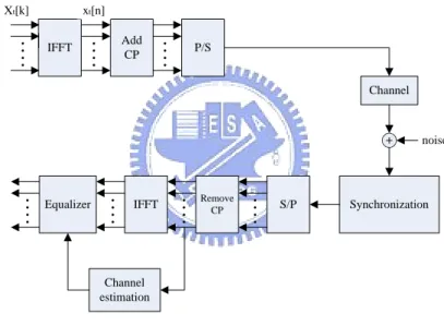
2.1 System model
Consider an OFDM system with N subcarriers signaling through a time-varying frequency-selective Rayleigh fading channel. The whole system in base band model is illustrated in Fig.1. Synchronization S/P Remove CP IFFT Equalizer noise Channel Channel estimation Add CP IFFT P/S Xt[k] xt[n]
Fig. 1 System model
The data are modulated in blocks by means of a discrete Fourier transform (DFT),given by
[ ]
[ ]
1 0 2 exp 0 , 1 (2.1) N t t k kn x n X k j n k N N π − = ⎛ ⎞ = ⋅ ⎜− ⎟ ≤ ≤ − ⎝ ⎠∑
where the subscript t represents the OFDM frame. A cyclic prefix (CP) is inserted into
the transmitted signal to prevent the intersymbol interference (ISI) between successive OFDM frames. After parallel to serial conversion, the signals are transmitted trough a frequency selective time-varying fading channel. At the receiver side, the received time-domain signal can be expressed as [15]
th
[ ]
1[ ]
, 0 0 1 (2.2) L t t n l t N t l r n h x n l n n n N − = ⎡ ⎤ =∑
⋅ ⎣ − ⎦+ ≤ ≤ −where represents the channel impulse response (CIR) of the path during OFDM
frame, L represents the length of the frequency-selective fading channel,
, t n l h lth tth
[ ]
t n n representsthe additive white Gaussian noise (AWGN) with zero mean and variance
[ ]
2 2t
E n n⎡⎢⎣ ⎤ =⎥⎦ σ , and
N
i represents the modulo-N operation. The fading channel coefficients are
modeled as zero mean complex Gaussian random variables. According to Wide Sense Stationary Uncorrelated Scattering (WSSUS) assumption, the fading coefficients in different delay paths are statistically independent. In the time domain, the fading
coefficients are correlated and have a Doppler power spectrum density modeled as in
Jakes [16], given by , t n l h , t n l h 2 1 ( ) 1 (2.3) otherwise 0 d d d f F f D f F F π ⎧ ⎪ ≤ ⎛ ⎞ ⎪ =⎨ −⎜ ⎟ ⎝ ⎠ ⎪ ⎪ ⎩
where Fd is the Doppler bandwidth. Hence hn lt, has an autocorrelation function given by
(
)
(
)
, , 0 E hn lt hm lt J 2π n m F Td s (2.4) ∗ ⎡ ⋅ ⎤= − ⎣ ⎦where J0
( )
i is the first kind Bessel function of zero order and T is OFDM sample sduration.. Then substitute equation (2.1) into (2.2):
[ ]
1 1[ ]
,(
)
[ ]
0 0 2 1 exp 0 1 (2.5) L N t t t n l t l k k n l r n X k h j n n n N N N π − − = = ⎛ − ⎞ = ⋅ ⎜ ⎟+ ≤ ≤ − ⎝ ⎠∑∑
[ ]
{ }
[ ]
[ ]
1 1 1[ ]
,(
)
[ ]
0 0 0 2 1 exp 0 1 (2.6) t n t N L N t t n l n l k t t Y m DFT r n k n l mn X k h j w n n N N N Y m π − − − = = = = ⎛ ⎡⎣ − + ⎤⎦⎞ = ⋅ ⎜⎜ ⎟⎟+ ≤ ≤ − ⎝ ⎠∑∑∑
Where Y m represent the received signal at the t
[ ]
subcarrier of the OFDM frameand
th
k tth
[ ]
t
w n is i.i.d complex AWGN noise due to the orthonormal transformation of the
original noise n nt
[ ]
. It also can be written in a concise matrix form as
Yt =H Xt⋅ t+Wt (2.7)
where Yt and Wt are vectors of sizeN× , and the channel matrix H1 t is given by
(
)
1 1 , , , 0 0 2 1 , exp (2.8) N L t t t p q N N p q n l n l q p n ql H H h j N N π − − × = = ⎛ ⎡⎣ − − ⎤⎦⎞ ⎡ ⎤ =⎣ ⎦ = ⎜⎜ ⎟⎟ ⎝ ⎠∑∑
t H2.2 Inter-carrier interference in OFDM systems induced by the Doppler effect
OFDM is robust against frequency selective fading due to the increase of the symbol duration. With the introduction of the CP, the problem of the ISI in single-carrier systems can be greatly reduced. However, in mobile radio environment, multipath channels are usually time-varying. Channel variations within an OFDM block destroy the orthogonality among the subcarriers, resulting in ICI and performance degradation. Since the transmitted symbol duration is N times longer than that in a single-carrier system, the increase in the symbol duration makes the system more sensitive to the time variation of the channel. If ICI is modeled as an additive white Gaussian process and not adequately compensated, the
ICI will lead to an error floor. Doppler frequency is used to indicate the rate of the
channel variation, which is proportional to vehicle velocity and carrier frequency
d
F
v f , c
c (2.9) d v f F c ⋅ =
Therefore, the ICI induced by time-varying channel is determined by Doppler frequency
and the OFDM symbol duration . In order to analyze the symbol energy distribution
and ICI on one subcarrier, equation (2.6) can be modified as following form
d F T
[ ]
[ ]
1[ ]
[ ]
, , 0, 0 1 (2.10) N t t t m m t m n t t n n m Y m H X m H X m w n m N − = ≠ = +∑
+ ≤ ≤ −The first term in (2.10) is the desired signal, the second term represents the ICI from the other subcarriers, and finally the third term is the additive noise. Hence, the energy of
[ ]
t
X n leaked to the mth subcarrier can be expressed as
[ ]
(
) (
)
(
)
2 * , , , , 1 1 1 1 * , ', ' 2 0 0 ' 0 ' 0 1 0 2 , , 0 ' 0 2 exp ' ' ' (2.11 ) 2 ' t t t m n m n t s m n m n N L N L t t s k l k l k m l k l N N s s d k m n k n P P E H X n E E H H E E h h j l k l k n k k m N N E T J F k k N N P π π − − − − = = = = − = = ⎡ ⎤ ⎡ ⎤ = ⎢ ⎥= ⎣ ⎦ ⎣ ⎦ ⎛ ⎞ ⎡ ⎤ ⎡ ⎤ = ⎣ ⎦ ⎜− ⎣ − − + + − ⎦⎟ ⎝ ⎠ ⎛ ⎞ = ⎜ − ⎟ ⎝ ⎠∑∑∑∑
∑
(
)(
)
1 2 exp j k' k n m Pl N π − ⎛ ⎞ − − − = ⎜ ⎟ ⎝ ⎠∑
where Es =E X n[ t[ ]
2] and l= − n mThe energy of X n distributed to subcarrier t
[ ]
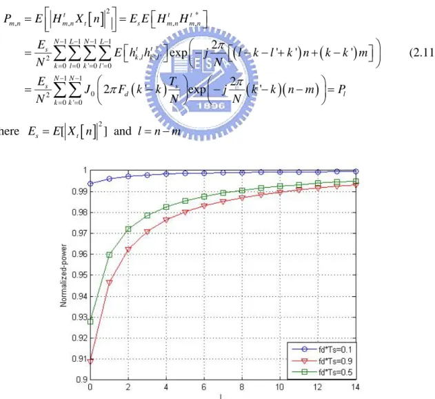
n v− to n v+ can be expressed as(
)
(
)
1 1 0 2 0 ' 0 2 ' 2 ' exp( ) (2.12) v N N v s s v l d l v k k l v k k l E T P J F k k j N N N π π − − =− = = =− − ⎛ ⎞ Φ = = ⎜ − ⎟ − ⎝ ⎠∑
∑∑
∑
The normalized symbol energy distributionΦv Es is depicted in Fig. 2. It indicates that most of the subcarrier’s energy is spread over itself and its nearby subcarriers when f Td s < , 1 and more than 99% of the subcarrier’s energy is distributed on itself and its two nearby
subcarriers when . Therefore, the ICI on one subcarrier mostly comes from only
few neighborhood subcarriers. 0.1
d s
f T =
Chapter 3
ICI Mitigation in Doppler Spread Channel
3.1 Pilot-based channel estimation
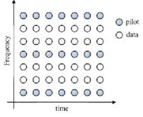
Pilot-based approaches are widely used to estimate channel properties and correct the received signal [14]. Usually, a comb-type pilot subcarriers arrangement is adopted, as depicted in Fig. 3. For each transmitted symbol, pilot signals are uniformly distributed within an OFDM symbol, while null and data tones are assigned to other subcarriers.
Fig. 3 Comb-type pilot arrangement
Without using any knowledge of statistics of the channels, the estimate of the channel at pilot subcarriers based on least square (LS) estimation is given by
[ ]
[ ]
[ ]
ˆ [ ] (3.1) p p p p Y m H m P m N Y m Y m N = ⎡ ⎤ = ⎢ ⎥ ⎢ ⎥ ⎣ ⎦ m=0,1, 2 ,Np−1whereNis the number of subcarriers, Npis the number of pilot subcarriers andP m is the
[ ]
interpolation technique in order to obtain the channel information at null and data subcarriers. Before further discussion, assume that the number of pilots is large enough such that aliasing of channel impulse response will not occur. The channel estimation at the
p
N m l
N + -th subcarrier using linear interpolation is given by [17]
(
)
(
(
)
)
ˆ ˆ ˆ 1 ˆ 1 1 (3.2) p p p p p p p p p N N N N N H m l H m H m H m l N N l N N N N N ⎛ ⎞ ⎡ ⎤ ⎡ ⎤ ⎡ ⎤ ⎡ ⎤ + = +⎜ + − ⎟ ≤ ≤ − ⎢ ⎥ ⎢ ⎥ ⎜ ⎢ ⎥ ⎢ ⎥⎟ ⎢ ⎥ ⎢ ⎥ ⎢ ⎥ ⎢ ⎥ ⎣ ⎦ ⎣ ⎦ ⎝ ⎣ ⎦ ⎣ ⎦⎠The second-order interpolation performs better than the linear interpolation method, where channel estimates at the data subcarriers are obtained by weighted linear combination of the three adjacent pilot estimates, given by [7]
(
)
(
)
(
)
(
)(
)
(
)
1 0 1 1 0 1 ˆ ˆ 1 ˆ ˆ 1 1 2 1 1 , = 1 2 p p p p p p p N N N N H m l c H m c H m c H m N N N N c l where c N c α α α α α α α − − ⎡ ⎤ ⎡ ⎤ ⎡ ⎤ ⎡ ⎤ + = − + + + ⎢ ⎥ ⎢ ⎥ ⎢ ⎥ ⎢ ⎥ ⎢ ⎥ ⎢ ⎥ ⎢ ⎥ ⎢ ⎥ ⎣ ⎦ ⎣ ⎦ ⎣ ⎦ ⎣ ⎦ ⎧ − = ⎪ ⎪⎪ = − − + ⎨ ⎪ + ⎪ = ⎪⎩ (3.3)The low-pass interpolation method is performed by inserting zeros into the LS estimates at pilot subcarriers and then applying a low-pass finite-length impulse response (FIR) filter, which allows the original data to pass through unchanged and interpolates such that the mean-square error (MSE) between the interpolated points and their ideal values is minimized. The time domain interpolation [4] is a high-resolution interpolation based on zero-padding and DFT/IDFT. First, it converts Hˆp
[ ]
m to time domain by IDFT :[ ]
1[ ]
0 2 exp( ) 0,1, 1 (3.4) p N p p p k p kn G n H m j n N N π − = =∑
= −Then, based on the basic multi-rate signal processing properties, the -sample time
domain sequence
p
N
[ ]
p
p
N−N zeros samples at the “high frequency” region around Np 2, given by
[ ]
[ ]
0 2 0 (3 2 2 p p p p N N G q q N N G q q N ≤ ≤ = < ≤ − .5) 1 2 2 p p p N N G q N N q N ⎧ ⎪ ⎪ ⎪ ⎨ ⎪ ⎡ ⎤ ⎪ − + − < ≤ − ⎢ ⎥ ⎪ ⎣ ⎦ ⎩Finally, the estimate of the channel at all frequencies is obtained by:
[ ]
1[ ]
0 2 exp( ) 0 1 (3.6) N N n nk H k G n j k N N π − = =∑
− ≤ ≤ −The performance among the comb-type estimation techniques usually ranks from the best to the worst as follows: low-pass, time-domain, second-order, and linear.
3.2 The proposed method
First we will recapitulate why the LS estimator presented in the previous section is not adequate at combating ICI. The LS estimator with 1-D interpolation compensates for the frequency-selectivity fading channel, assuming that the channel is stationary during one
symbol interval. Usually, if f T is les than 0.01, the channel can be assumed constant d
during one symbol interval. But the equalizer considers the ICI as an additive Gaussian random process, the performance of equalizer degrades significantly due to ICI for larger channel variation, as for f Td ≥0.01.
To fully count the ICI effect, (2.7) should be used to solve , and it is necessary to
estimate the channel matrix then calculate its matrix inverse. Nevertheless, accurate
estimation of the transfer function requires complete knowledge of the time-variation of the CIR for each OFDM symbol, which is not usually available. When the OFDM symbol duration is smaller than 10% of the channel coherence time, the variation of the channel during a block period can be assumed in a linear model [10]. By utilizing the above
t
X
t
assumption, the estimation problem of the channel matrix can be greatly simplified, since the value of the slope of the linear model uniquely determines the ICI. The
component of the channel matrix can be expressed as
t H t H
(
)
(
)
(
)
(
)
(
)
, 1 1 , , 0 0 1 1 , 0 0 1 1 1 0 0 0 1 2 exp 1 2 exp 2 2 1 2exp exp exp(
N L t t p q n l n l N L l l n l L N p q q N l l k p l k H h j p q n ql N N a n b j p q n ql N N p q n p q n ql a j b k j j N H N H N π π π π π − − = = − − = = − − − = = = ⎛ ⎡ ⎤⎞ = ⎜− ⎣ − + ⎦⎟ ⎝ ⎠ ⎛ ⎡ ⎤⎞ = + ⋅ ⎜− ⎣ − + ⎦⎟ ⎝ ⎠ ⎛ ⎛ − ⎞ ⎛ − ⎞⎞ = ⎜⎜ ⋅ ⎜− ⎟+ ⋅ ⎜− ⎟⎟⎟ − ⎝ ⎠ ⎝ ⎠ ⎝ ⎠
∑∑
∑∑
∑
∑
∑
, ) (3.7) p q 1 2 p=q 2 q p q p q q q ql j N H N B N A B π − ⎛− ⎞ ⎜ ⎧ ⎫ Φ ≠ ⎪ ⎪ ⎪ ⎪ = ⎨ ⎬ − ⎪ + ⎪ ⎪ ⎟ ⎝ ⎩ ⎭ ⎠ ⎪ where 1 0 1 0 2 exp( ) 2 exp( ) (3.8) 1 2 exp( ) 1 L q l n L q l n q ql A a j N ql B b j N q j N π π π − = − = = − = − Φ = − −∑
∑
It is shown in (3.7) that the main diagonal of the estimated channel matrix depends on the average of the channel frequency response during one block period and the ICI term is only determined by the channel variation and OFDM parameters. Then substitute (3.7) and (3.8) into (2.7),we get
[ ] [ ] [ ] 1 1 0 0 0 1 2 1 1 1 1 2 1 0 0 0 0 2 0 1 1 0 0 0 1 2 (3.9) N N N N N N N N X A B B X A Y N N B B X N − − + − + − − − − − − Φ Φ + ⋅ Φ Φ = + + − + ⋅ Φ Φ − ⎧⎛ ⎞ ⎛⎛ ⎞⎞ ⎫⎛ ⎞ ⎜ ⎟ ⎪ ⎜⎜ ⎟⎟⎛ ⎞⎪⎜ ⎟ ⎪⎜ ⎟ ⎜⎜ ⎟⎟⎜ ⎟⎪⎜ ⎟ ⎨⎜ ⎟ ⎜ ⎟⎬ ⎜⎜ ⎟⎟⎜ ⎟ ⎜ ⎟ ⎪⎜ ⎟ ⎜⎜ ⎟⎟⎝ ⎠ ⎜⎪ ⎟ ⎪⎜ ⎟ ⎝⎝ ⎠⎠ ⎪⎝ ⎠ ⎩⎝ ⎠ ⎭ t t t Y = H X + N … … i i
Since only depends on OFDM parameters, it is possible to precalculate it once at initialization. There are several schemes proposed in the following. The procedure for the estimation of the channel matrix is shown in Fig. 4 and described as follows.
q
Φ
Fig. 4 Block diagram of the estimation of the channel matrix
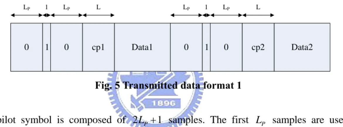
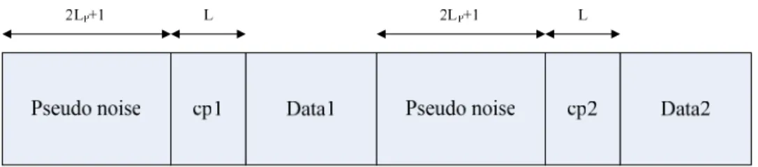
First, a time domain pilot signal is inserted at the end of every symbol, as shown in Fig. 5. A similar method can be found in [10].
0 1 0 cp1 Data1 0 1 0 cp2 Data2
LP 1 LP L LP 1 LP L
Fig. 5 Transmitted data format 1
The pilot symbol is composed of 2LP+ samples. The first 1 L samples are used to P
avoid ISI, while remaining LP+ samples are inserted for CIR estimation. Then, by 1
comparing the CIR changes between the received signals corresponding to the (i−1)th
pilot symbol and th pilot symbol for each path, the CIR variation during the block period is estimated using linear interpolation. Although using pseudo-delta function to do the channel estimation is straightforward, it may have some drawbacks. In order to coincide with the signal power spectrum density, the pseudo-noise can be used as time domain pilot in place of the delta function, as shown in Fig.6.
Fig. 6 Transmitted data format 2
Before further discussion, we assume that the length of time domain pilot is M- sample.
Assuming the channel variation during the M samples can be negligible. The time
domain convolution can be expressed as a matrix vector multiplication. The linear
convolution matrix is formed from the time domain pilot.The least-square channel estimate, assuming P PH has full rank, is given by
(
)
ˆ
h = P PH -1P rH (3.10)
and the corresponding MSE is given byσn2tr
{
(
P PH)
−1}
. Based on minimizing the channelestimation MSE, it can be achieved if and only if has equal eigenvalues. This is
achieved when
H
P P
P P =H EPI (3.11)
where denotes the linear convolution matrix. It can be observed that the time domain pilot
should be a shift-orthogonal sequence. The corresponding minimum MSE is
P
2
n P
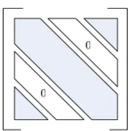
Lσ E . Then, the CIR variation for each path during the OFDM symbol can be estimated with linear interpolation, given the LS estimates at the inserted pilot symbols. Finally, the proposed method reconstructs the channel matrix and calculates its matrix inverse. Since the channel matrix can have a large size, it is difficult to process in real time. Based on the
structure of the channel matrix , whose energy is concentrated on the neighborhood of
the main diagonal, the computation complexity can be reduced by considering only the elements nearby the main diagonal and ignoring remaining elements, as shown in Fig. 7.
t
Fig. 7 Banded channel matrix with color region corresponding to ICI concentration
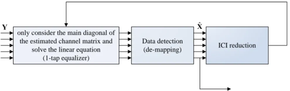
Another way to avoid straight matrix inversion is to divide the task into ICI reduction and a simple one-tap equalizer. In the following, the ICI reduction procedure will be described in detail. According to equation (2.7), it can be found that ICI component is determined by not only the variation of the channel but also the transmitted data. The decision-feedback techniques can be utilized to acquire the estimates of the transmitted data, then the estimated channel matrix in (3.9) is used to subtract the ICI components from the received signal. The resulting ICI reduction method is as follows
[ ]
[ ]
[ ]
[ ]
[ ]
1 , 0, m,m ˆ ˆ 0 1 (3.12) 1 ˆ =Dec ˆ H N t t t m n t n n m t t Y m Y m H X m m N X m Y m − = ≠ = − ≤ ≤ − ⎛ ⎞ ⎜ ⎟ ⎜ ⎟ ⎝ ⎠∑
(3.13)where Dec denotes a slicer in the demapper. Assuming that the number of data carriers is large, the effect of incorrect hard decisions will not have a significant impact. Finally, the ICI-cancelled Y m can be used in a conventional one-tap equalizer. For severe Doppler t
[ ]
effects, it also can be combined with an iterative method to enhance the ICI estimation accuracy, as shown in Fig. 8. In addition, the hard decision in (4.1) can be replaced by a MMSE equalization, given by
[ ]
*m,m[ ]
2 m,m ˆ H ˆ = (3.14) ˆ H 1/ t t Y m X m SNR +only consider the main diagonal of the estimated channel matrix and
solve the linear equation (1-tap equalizer)
Data detection
(de-mapping) ICI reduction
ˆ
X Y
Fig. 8 Block diagram of the proposed ICI-reduction method
In the same manner, the computation complexity of the ICI reduction can be reduced
by considering only the ICI component due to the nearby subcarriers without degrading
much system performance, given by
q
[ ]
[ ]
1 ,[ ]
0, 2 ˆ ˆ 0 1 (3.15) N t t t m n t n n m q Y m Y m H X m m N − = − ≤ = −∑
≤ ≤ −Even, it can be ignored the off-diagonal elements of the estimated channel matrix and use one-tap equalizer without ICI reduction. It can be observed in (3.7) that the main diagonal elements are the average of the channel frequency response during one block period. Based the linear property, it can be obtained by
1 ( ) (3.16) 2 t t N h h diag =DFT ⎧⎨ + + ⎫⎬ ⎩ ⎭ t Η
where the subscript denotes the OFDM frame and denotes the main diagonal
of the matrix. Then, utilize one-tap equalizer without ICI reduction.
t tth diag()
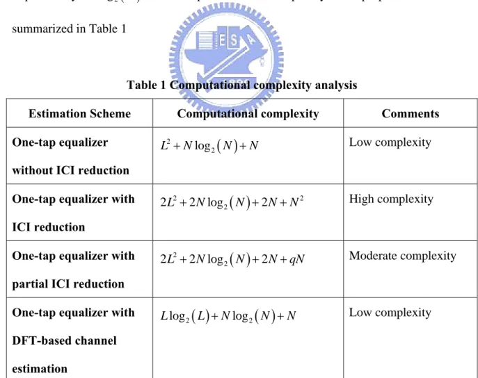
3.3 Computation complexity analysis
Utilizing the time domain pilot inserted at the end of every OFDM symbol to acquire
the time domain channel estimates in (3.10) requires multiplications. The matrix can
be pre-calculated at the initialization. Based on the linear property of the channel variation, the computation of the channel matrix in (3.8) and (3.9) approximately requires
2
( )
22Nlog N
)
N
multiplications. The method that directly uses the inversion of the estimated
channel matrix requires computational complexity. The method using one-tap
equalizer with ICI reduction approximately requires
multiplications. The simplified method in (3.14) and (3.15) using one-tap equalizer with ICI reduction which only consider the elements of the estimated channel matrix in the adjacent of the main diagonal requires
3 ( O N
( )
2 2 2Nlog N +2N+( )
2 2Nlog N +2N+ Nq Nmultiplication. As the size of the channel matrix increases, the simplified method conserves more computation complexity than that of which utilizes the whole estimated channel matrix to do ICI-reduction. The method using one-tap equalizer without ICI reduction approximately
requires only multiplication. The complexity of the proposed methods are
summarized in Table 1
( )
2log
N N +
Table 1 Computational complexity analysis
Estimation Scheme Computational complexity Comments One-tap equalizer
without ICI reduction
( )
22
log
L +N N + N Low complexity
One-tap equalizer with ICI reduction
( )
22
2L +2Nlog N +2N+N2 High complexity
One-tap equalizer with partial ICI reduction
( )
22
2L +2Nlog N +2N+qN Moderate complexity
One-tap equalizer with DFT-based channel estimation
( )
( )
2 2 log log L L +N N + N Low complexityChapter4
Simulations and Discussions
4.1 Simulation result
1) System parameters:
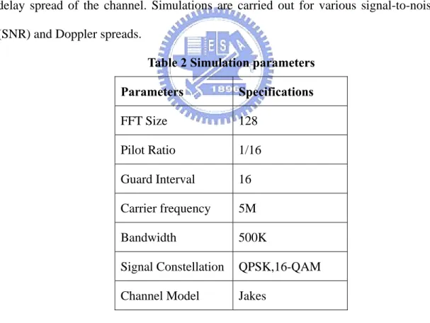
OFDM system parameters used in the simulations are illustrated in Table 2. Since the aim is to observe channel estimation performance, it assumed to be perfect synchronization in the simulations. Moreover, the guard interval is assumed to be longer than the maximum delay spread of the channel. Simulations are carried out for various signal-to-noise ratio (SNR) and Doppler spreads.
Table 2 Simulation parameters
Parameters Specifications FFT Size 128 Pilot Ratio 1/16 Guard Interval 16 Carrier frequency 5M Bandwidth 500K
Signal Constellation QPSK,16-QAM
Channel Model Jakes
2) Channel model
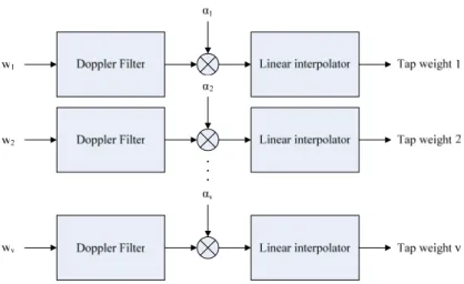
Assume a symbol spaced, tap-delay-line channel model of 4 paths, where each channel tap is generated with the Doppler spectrum based on the Jakes’ model. The
generation of the tap gains is illustrated in Fig. 9.
Fig. 9 Generation of the tap weight processes
It start with a set of independent, zero-mean complex Gaussian white noise processes, which are filtered to produce the appropriate Doppler spectrum, as depicted by the Jakes model. These are then scaled to produce the desired power profile. In the simulations, the path gains follow the exponentially-decayed power profile as depicted by
( )
2 (4.1) l l E t e τ σ α − ⎡ ⎤ = ⎢ ⎥ ⎣ ⎦where αl
( )
t is the path gain, τl is the path time delay and σ is the power delayconstant. We choose the power delay time constant such that the last path power is 20dB below the first path. Before further discussion, we assume the overhead of the proposed method and DFT-based method are the same. Moreover, the suboptimal time domain pilot we used is the product of the shift-orthogonal sequence and a finite-duration window function, such as Hanning window.
Fig. 10 shows the BER performance for the case f Td s =0.04. The modulation scheme
used for this simulation is 16-QAM. Assume the pilot subcarriers are equispaced along the frequency domain such that DFT-based channel estimator can be used. The DFT-based channel estimation is also shown as reference, which has comparable performance to that of MMSE channel estimation method. In addition, the overhead of the proposed method are
the same as that of the DFT-based method in the simulation. From Fig. 13, it can be observed that the ICI-reduction algorithm effectively reduces the error floor, as is more evident especially in high SNR than low SNR. The method using the one-tap equalizer with ICI reduction has comparable performance to that of directly using the inversion of the estimated channel matrix, while costs much less computation.
Fig. 10 BER performance of ICI reduction algorithm with f Td s =0.04
Fig. 11 also shows the BER performance for the case with choosing
different number of the nearby subcarriers for ICI reductions. From Fig. 11, it can be
observed that the simplified scheme gives comparable results to the method using whole estimated channel matrix but has low computation complexity.
0.04
d s
f T =
q
Fig. 12 and Fig.13 shows the BER performance respectively for the case f Td s =0.1.
and . From Fig.12, it can be observed that the proposed method From Fig.13, it
can be observed that the proposed method gives rise to an error floor as the assumption of the linear property of the channel variation no longer holds.
0.2
d s
f T =
Fig. 14 and Fig. 15 shows the BER performance for the case f Td s =0.04
respectively under various conditions of carrier frequency offset and timing offset . From Fig. 14, it can be observed that the proposed method is robust to the effect of carrier frequency offset. From Fig. 15, it can be shown that the proposed method is sensitive to the timing offset.
Fig. 13 BER performance of ICI reduction algorithm with f Td s =0.2
Fig. 15 BER performance of proposed method with f Td s =0.04 and various timing
offset
Consider that the tolerance interval to symbol timing error is samples and the maximum
channel length is
k
L. The comparison among the proposed methods and DFT-based method
are summarized as in Table 3, including overhead, computational complexity and BER performance.
From Table 3, it can be concluded that the overhead of the proposed method is slightly more than that of the DFT-based method but the performance of the proposed method is much better than that of the DFT-base method. Moreover, it is worthwhile to increase the computational complexity for the sake of performance, as shown in Table 3.
Table 3 Overhead, complexity and performance of the various schemes
Estimation Scheme Overhead Complexity Performance
One-tap equalizer without ICI reduction
Moderate
(2L+3K−1)
Low Moderate
One-tap equalizer with ICI reduction
Moderate
(2L+3K−1)
High Very good
One-tap equalizer with partial ICI reduction
Moderate
(2L+3K−1)
Moderate Very good
One-tap equalizer with DFT-based method
Low
(2L+2K−1)
4.2 Conclusion
Usually, DFT-based receivers considers ICI as an additive noise and it is not adequately compensated. In this thesis, we propose the time domain pilot-based estimation scheme combined an iterative method to suppress the ICI induced by time varying channels. It is shown through simulation that ICI can be compensated by the proposed method if the normalized Doppler frequency change is in the range of ( 0.01≤ f Td s ≤0.1). The reason is that for the channel with a very high Doppler frequency, the assumption that the channel parameters vary in a linear fashion within a block period is no longer a good approximation and gives rise to an error floor. On the other hand, the channel can be assumed invariant during a block period if the normalized Doppler frequency less than 0.01.Under these circumstances, the proposed method only slightly outperforms the DFT-based method. Furthermore, we also proposed a simplified method using a one-tap equalizer with partial ICI reduction; it has comparable performance to that using whole estimated channel matrix for ICI reduction.
Reference
[1] A.A. Hutter, R. Hasholzner, and J.S. Hammerschmidt, “Channel estimation for mobile OFDM systems,” Proc. IEEE VTC’99-Fall, Sept. 1999.
[2] J. Armstrong, P. M. Grant, and G. Povey, “Polynomial cancellation coding of OFDM to reduce intercarrier interference due to Doppler spread,” in Proc. IEEE Global
Telecommunications Conf., vol. 5, pp. 2771-2776, 1998
[3] A. Seyedi, and G.J. Saulnier, “General self-cancellation scheme for mitigation of ICI in OFDM systems,” IEEE Communications Conf., VOL. 5, PP. 2653-2657, June 2004.
Communication Systems Based on Pilot Signals and Transform-Domain Processing,” Proc. VTC’97, pp. 2089-2094
[5] Y.-S. Choi, P. J. Voltz, and F. A. Cassara, “On channel estimation and detection for multicarrier signal in fast and selective Rayleigh fading channels, ” IEEE Trans. Commun., vol. 49, pp. 1375-1387, Aug. 2001.
[6] O. Edfors, M. Sandell, J.-J. van de Beek, S. K. Wilson, and P. O. Brjesson, “OFDM channel estimation by singular value decomposition,” IEEE Trans. Commun., vol. 46, no. 7, pp. 931–939, Jul. 1998.
[7] Coleri, S. Ergen, M., Puri, a., and Bahai, A., “Channel Estimation Techniques Based on Pilot Arrangement in OFDM Systems,” IEEE Transactions on Broadcasting, vol. 48,pp. 223-229, Sept. 2002.
[8] P. Robertson, and S. Kaiser, “Analysis of the loss of orthogonality through Doppler spread in OFDM systems,” IEEE Globecom., vol. 1B, pp. 701-706, Dec. 1999.
[9] W. G. Song, and J. T. Lim, “Pilot-symbol aided channel estimation for OFDM with fast fading channels,” IEEE Transactions on Broadcasting, vol. 49, no. 4, Dec. 2003
[10] W.G. Jeon, K. H. Chang, and Y. S. Cho, “An Equalization Technique for Orthogonal Frequency-Division Multiplexing Systems in Time-Variant Multipath Channels,” IEEE
Trans. Commun., vol.47, no. 1, Jan. 1999.
[11] P. Chen, and H. Kobayashi, “Maximum Likelihood Channel Estimation and Signal Detection for OFDM systems,” IEEE ICC, vol. 3, pp. 1640-1645, 2002.
[12] K. A. D. Teo, and S. Ohno, “Pilot-Aided Channel Estimation and Viterbi Equalization for FODM over Doubly-Selective Channel,” IEEE Globecom., Nov. 2006.
[13] S. He, J. K. Tugnait, “Doubly-Selective Channel Estimation Using Superimposed Training and Discrete Prolate Spheroidal Basis Models,” IEEE Globecom., Nov. 2006 [14] A. Bourdoux, F. Horlin, E. L. Estraviz, and L. V. der Perre, “Practical Channel Estimation for OFDM in time-varing channels,” IEEE Globecom., Nov. 2006.
Interference in OFDM Systems,” in Proceedings of the IEEE WCNC, vol. 1, (New Orleans), pp. 39-44, Mar. 2005.
[16] W.C. Jakes, Microwave Mobile Communications, IEEE Press, Reprinted, 1944. [17] L. J. Cimini, “Analysis and simulation of a digital mobile channel using orthogonal frequency division multiplexing,” IEEE Trans. Commun., vol. 33, no. 7, pp. 665-675, Jul. 1985.