A New Sequential Diagnosis Algorithm in Hypercubes with High Diagnosability

全文

(1)Int. Computer Symposium, Dec. 15-17, 2004, Taipei, Taiwan.. A New Sequential Diagnosis Algorithm in Hypercubes with High Diagnosability Yao-Ming Chang, Yao-Ming Yeh Department of Information & Computer Education National Taiwan Normal University, Taipei, Taiwan E-mail: { lming, ymyeh }@ice.ntnu.edu.tw Deterministic diagnosis methods are defined as those methods, in which the entire fault set (or a well defined subset of the fault set) can be uniquely identified from the syndrome provided that certain assumptions on the structure of the testing graph and the behavior of faulty and non-faulty nodes are satisfied. By contrast, probabilistic diagnosis methods [6] that only attempt to correctly diagnose faulty nodes with high probability and require no restrictive assumptions on the structure of the testing graph. In the deterministic diagnosis methods, which are the concern in this paper, a certain restriction is imposed on the faulty hypercube systems, such as diagnosability. The diagnosability of a system under the selected diagnosis strategy is the maximum number of faulty nodes that can exist in a system at any given time without invalidating the diagnosis strategy. Thus a system is said to be t-diagnosable if all faulty nodes within the system can be identified that the number of faulty nodes does not exceed t. A large number of extensions of PMC model have been proposed in order to expand the range of applicability of the diagnosis model. These includes one-step [11], pessimistic [4, 14], adaptive [12, 13] and sequential [1, 3, 5-7] diagnosis strategies. The efforts of one-step diagnosis (or diagnosis without repair) are made to locate all faulty nodes in one test phase, and thereafter the repair phase, in which all identified faulty nodes are repaired follows. Later Friedman and Kavianpour [14] proposed a strategy under which a set of fewer nodes containing all faulty nodes and possibly some nodes of unknown status were identified and repaired. This strategy is called a pessimistic diagnosis strategy. In adaptive diagnosis, the next test can be determined after seeing the result of previous ones. The adaptive diagnosis of the hypercube systems was studied in [12] for the first time. Instead of higher diagnosability, the object of adaptive diagnosis is to minimize the number of tests and the number of testing rounds. Sequential diagnosis is also known as diagnosis with repair [1] done in stages with previously identified faulty nodes replaced at each stage. Since one-step diagnosability of a system is limited above by the minimum of the node in-. Abstract-We consider the problem of sequential fault diagnosis in hypercube multiprocessor system under the PMC model. The diagnosability is defined as the ability to provide a correct and complete diagnosis. In this paper, we proposed a novel and simple sequential diagnosis method called the Major Aggregate (MA) Algorithm. Moreover, the lower bound of diagnosability in our method is proved as. ⎛ 2d ⎞ ⎟⎟ of a d-dimensional hypercube. This result Ω⎜⎜ ⎝ d⎠ obviously improves the best lower bound of diagnosability,. ⎛ 2 d log d ⎞ ⎟⎟ , Ω⎜⎜ d ⎝ ⎠. in. previous. researches.. 1. Introduction Large multiprocessor systems play a getting important role in high-performance computing. Meanwhile, it becomes an important issue to develop practical techniques for the fault diagnosis of such systems. System-level fault diagnosis is to identify faults in a system to the processor level. The systemlevel diagnosis has been extensively studied in the literature in connection with fault-tolerant multiprocessor systems. An original graph-theoretical model, as well as PMC model for system diagnosis, which have been introduced by Preparata, Metze and Chien [1]. Adapting this model to the hypercube systems, each node can test all its neighboring nodes to determine whether they are faulty or non-faulty from its own viewpoint. A non-faulty testing node always gives reliable test results, whereas a faulty one provide any test results regardless of the status of the tested node. A set of test results is called the syndrome of the system. For global diagnosis, all the syndromes are gathered by a special monitoring processor, which is called syndrome analyzer and proceeds to determine the status of all nodes on this basis. The currently available methods for systemlevel diagnosis can be broadly categorized into deterministic and probabilistic methods.. 1244.

(2) Int. Computer Symposium, Dec. 15-17, 2004, Taipei, Taiwan.. degrees [1], sequential diagnosis is more feasible under realistic fault situations. Sequential diagnosis of hypercubes has been addressed in several papers. In [5], Kavianpour and Kim presented a sequential diagnosis strategy that the diagnosability of this strategy is. (. ). t ∈ Θ d ⋅ 2 d . Khanna and Fuchs [7] introduced a cluster-based sequential diagnosis algorithm for hypercubes. The algorithm also has diagnosability. (. t ∈ Θ d ⋅ 2d. ).. In [6], the same authors introduced the PARTITIOIN sequential diagnosis algorithm for regular graphs. When it applied to. ⎛ 2 d log d ⎞ ⎟⎟ . ⎝ d ⎠. hypercubes, the diagnosability is t ∈ Ω⎜⎜. In this paper, we proposed a novel and simple sequential diagnosis method called the Major Aggregate (MA) Algorithm. Moreover, the lower bound of diagnosability in our method is proved as. return 1 (or 0), while the test outcome of tests performed by faulty nodes is arbitrary. The outcomes of the 2|E(G)| tests can be abstracted into a labeled undirected graph called the syndrome graph GS. Then V(GS) = V(G) and E(GS) simply consists of the edges in E(G) with labels. An edge(u, v) is labeled as “pass” if the outcome of u test v is 0 and vice versa. Similarly, an edge(u, v) is labeled as “fail” if both outcomes of that u and v test each other are 1. Any other edges are given label “conflict”. An aggregate A is a connected component of node set in the syndrome graph GS. An aggregate A is a P-aggregate if every edge in A is labeled as “pass”. Lemma 1 characterizes the important property of P-aggregate in the syndrome graph. Lemma 1. All nodes in a P-aggregate are either complete fault-free or complete faulty. Because both nodes on edge labeled as “pass” must be the same state, lemma 1 is immediately proved. Since all nodes in this connected component are in the same state, the cardinality of a P-aggregate provides significant information for diagnosis algorithms. For example in [6], Khanna and Fuchs applied the cardinality of P-aggregate to be the criterion of fault-free subset identification. The main idea of the PARTITION algorithm is that under the assumption of diagnosability t, actual number of faulty nodes |Vf(G)| will not exceed t (i.e. |Vf(G)| ≤ t). Therefore, if the cardinality of a P-aggregate is larger than the actual number of faulty nodes |Vf(G)|, then one can declare the whole nodes in this aggregate is fault-free. According to the analysis in the above section, the issue of these aggregate-based methods can be transferred to the problem of determining the bound of diagnosability. Khanna and Fuchs [6] derived a lower bound to diagnosability of hypercubes is. ⎛2 ⎞ ⎟⎟ of a d-dimensional hypercube. This result Ω⎜⎜ ⎝ d⎠ d. obviously improves the best lower bound of diagnosability in previous researches. The paper is organized as follows: In section 2, preliminary definitions are introduced. In Section 3, the lower bound of diagnosability is discussed and proved. We also presented a novel sequential diagnosis algorithm and the performance analysis. Section 4 describes the improvement and comparison of previous research. Finally, Section 5 draws some conclusions.. 2. Preliminaries A d-dimensional hypercube system or dhypercube for short is composed of 2d nodes and modeled as an undirected graph G. Each node u is labeled with a d-digits binary unique identifier. Nodes are connected based on the Hamming distance of their labels: edge(u, v) exists iff the Hamming distance of the labels of u and v is 1. We use V(G) and E(G) to represent the set of nodes and communication links respectively. In order to concisely represent the performance characteristics of our algorithm for a given graph, a three-tuple notation of the form <tF, tT, tI> is used where tF is a lower bound on the degree of diagnosability, tT is an upper bound on the testing and syndrome decoding time, and tI denotes an upper bound on the number of iterations of diagnosis and repair needed by the algorithm. In the PMC model [1], diagnosis is based on a suitable set of tests between adjacent nodes. For each edge (u, v) ∈ E(G), let node u and v perform tests on one another. It assumes that tests of faulty (or faultfree) nodes performed by fault-free nodes always. ⎛ N log d ⎞ t = δ ⋅⎜ ⎟ for a nonnegative δ < 1 and ⎝ d ⎠ sufficiently large N (N = 2d). Although this result is surprising high, the exact value of coefficient δ was not given and δ approaches to 1 only when N approaches infinity. Caruso et al. [2] went a step further to verify the same lower bound of diagnosability provided in [6]. They circumvented some difficulty of involved computational problems by devising approximations which rely on edgeisoperimetric inequalities of regular graphs.. 3. A New Sequential Diagnosis Algorithm We introduced here a nwe sequential diagnosis algorithm called the Major Aggregate (or MA). 1245.

(3) Int. Computer Symposium, Dec. 15-17, 2004, Taipei, Taiwan.. algorithm, which can obviously improve the diagnosability for hypercubes.. To illustrate our ideas, we define the major aggregate as follows,. 3.1. Vertex-isoperimetric inequality. Definition (major aggregate). Given a syndrome graph GS, a major aggregate AM is a P-aggregate with maximum cardinality.. Before introducing our algorithm, let us review an important theorem which determined the minimum number of boundary nodes to an aggregate. Given any u, v ∈ V(G), the distance between u and v is the length of the shortest path from u to v and is denoted d(u, v). Since G is undirected, d(u, v) = d(v, u) and d(u, v) can be used as a metric on G. Given any A ⊆ V(G), let d(A, v) = min{ d(u, v) : u ∈ A }. Observe that d(A, v) = 0 if and only if v ⊆ A.. In our method, we assume that the major aggregate is fault-free when the number of faulty nodes is less than t, where t is the upper bound to diagnosability. Following theorem 2 gives the precise value of t for our method: Theorem 2. Given a syndrome graph GS of a ddimensional hypercube (d > 4), if number of faulty. C dd / 2 (or 2 ⋅ C(dd−−11) / 2 ). Definition (vertex boundary). Given any A ⊆ V(G),. nodes is not greater than. the vertex boundary of A, denoted as ∂A , is defined as the set of vertices at distance at most 1 from A, formally, ∂A = { v ∈ V(G) : d(A, v) ≤ 1 }.. when d is even (or odd), then the major aggregate is fault-free. Proof: For demonstrating the proof clearly, we propose a problem in advance that given a set of faulty nodes F, how minimum the major aggregate, AM can be divided. If the min. |AM| > |F|, then AM must be fault-free. As we known in previous subsection, when the. Definition (vertex-isoperimetric inequality). A vertex-isoperimetric inequality for a graph G is defined by a function g(m) such that | ∂A | ≥ g(m) for any A ⊆ V(G) with |A| = m.. number of faulty nodes is. In general, many vertex-isoperimetric inequalities for a given graph G can be defined. A vertex-isoperimetric inequality for hypercubes has been derived in [15], [16], and is stated in the following theorem.. ⎧. ∑. r +1. i =0. a Hamming-sphere [15] and |A1| =. ∑. i =0. d −1. cardinality of major aggregate. Cid =. ∑. Cid . Since. can say that if the number of faulty nodes is not greater than the minimum cut-set, the major aggregate must be fault-free.. d −r −2 i =0. Cid is. C dd / 2 when d > 4. From the above deduction, we. 3.3. The MA Algorithm The procedure of MA algorithm is similar to the PARTITION algorithm introduced in [6] which is composed of two phases: fault-free subset identification and iterative diagnosis and repair. However phase 1 in MA algorithm differs from the identification fashion in [6] that only major aggregate is concerned but not the cardinality of Paggregate greater than (t + 1).. Therefore, the number of boundary node is also d. ( d / 2 ) −1 i =0. when A1 is. d. i=r +2. ∑. always greater than the number of faulty nodes. 2 d = C0d + C1d + ... + Cdd = ∑i = 0 Cid. ∑. C dd / 2 which. (d – 1), 2 ⋅ C( d −1) / 2 when d is odd. Moreover, the. the total number of nodes in a d-dimensional hypercube is 2d which can be represented by series of binomial coefficients as follows,. Crd+1 when |A2| =. ⎫ ⎬ . First of all, ⎭. is called the minimum even cut-set. In the same way, the number of minimum cut-set is exactly twice of. From theorem 1, the minimum number of. C. i =0. d i. 2) – 1 and the number of faulty node is. k ⎫ ⎧ r = max ⎨k ∈{1,..., d } : ∑ Cid ≤ m⎬ i =0 ⎭ ⎩. boundary nodes of aggregate A1 is. i =0. d i. we assume d is even. If we want the cardinality of major aggregate to be the minimum, two summation terms in braces should be equal. Therefore r = (d /. Cid , where. d r +1 r. d −r −2. r. ∑C , ∑C ⎩. aggregate is max .⎨. Theorem 1. Let G be the d-dimensional hypercube and let A ⊆ V(G), with |A| = m. Then, | ∂A | ≥. Crd+1 , the minimum major. Cid .. 3.2. Major Aggregate. 1246.

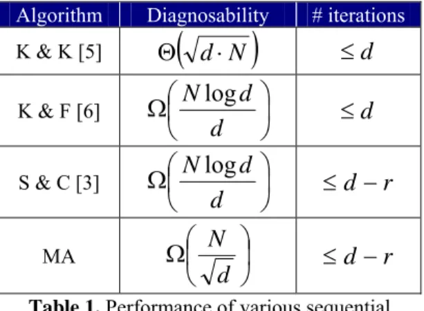
(4) Int. Computer Symposium, Dec. 15-17, 2004, Taipei, Taiwan.. Phase 1: Fault-free Subset Identification. The goal of this phase is to identify a subset of faultfree nodes. Each nodes test each one of its neighbors. The outcomes of these tests are used to form the syndrome graph GS. We do a depth-first search to locate the major aggregate, denotes as AM. Then all the nodes in this aggregate are guaranteed to be fault-free.. t1 1 2πd = = ……… (3) πd N π ⋅d /2 t log d π log d and 2 = = ……… (4) N d πd Because π is a constant, (3) is only related to. d and (4) is related to log d . As we known, when d grows lager, the value of (3) will increase faster than the value of (4). In the same way, we can calculate t1 / N of MA algorithm when d is odd. We use d = (2n + 1) in convenience:. Phase 2: Iterative Diagnosis and Repair. The goal of this phase is to iteratively diagnosis and repair faulty nodes. Select an arbitrary node, say u, from the AM identified in Phase 1 and then construct a breadth-first search tree of G rooted at this node. Let h denote the height of the tree, and let Li, 0 ≤ i ≤ h, be the set of nodes at distance i from u. Starting from the top of the tree, nodes in Li are used to diagnose nodes in Li+1. At step h, all the faulty nodes have been repaired.. d −1 t1 2 ⋅ C( d −1) / 2 2 ⋅ C n2 n (2n)! = = 2 n+1 = 2 n d N 2 2 2 ⋅ (n!) 2. ≈. Since n = (d – 1)/2, the above expression can be. 4. Comparisons. rewritten as. So far, the only known bound to the hypercube. ⎛ 2 d log d ⎞ ⎟⎟ , have be provided in d ⎠ ⎝. Theorem 3. The Major Aggregate Algorithm is a. [2] and [6]. For illustrating the comparison conveniently, we use t1 to denote the lower bound to diagnosability in our method and t2 to the previous d. best one. First of all, since t1 = C d / 2. =. ⎛ 2d ⎞ ⎟⎟ , O( d ⋅ 2 d ), d – r> sequential diagnosis < Ω⎜⎜ ⎝ d⎠. d! is (d / 2)!2. algorithm in hypercubes. Proof: First, the lower bound to diagnosability of MA algorithm was proved in the preceding paragraphs. Next, let us analyze the total testing and syndrome decoding time taken by the MA algorithm. The depth-first search in Phase 1 is easily seen to be performed in O( |E(G)| ) time. Since Phase 2 is the same as the algorithm in [6] and h ≤ d, the number of iterations needed to complete diagnosis is d in the worst case. However, Santi and Chessa in [3] proposed the i-PARTITION algorithm which improved the iterative diagnosis and repair phase (phase 2) of PARTITION algorithm that reduced the number of iterations needed to d – r, where r ∈ Θ(d ) . Therefore, the phase 2 can be rewritten same as in [3] to reduce the number of iterations. Table 1 shows the comparison result of various algorithms in asymptotic form. In addition, the lower bound provided by the algorithms also has been evaluated numerically. A listing for selected values of N (the size of the hypercubes) is reported as entry t1 in Table 2, along with the numerical evaluation of [6] (entry t2) and [2] (entry t3). It is seen that the lower bound to diagnosability of MA obviously improves the previous result.. an expression of factorials and not easy to compare with t2. We have to apply here the Stirling’s Formula [9] to reveal the approximation of factorials. From the Stirling’s approximation expression,. n!≈ 2πn ⋅ n n ⋅ e − n , we begin with calculating the ratio of t1 / N when d is even. For convenience to reduction, we use d = 2n to replace the parameter d d. in C d / 2 as follows:. t1 C dd / 2 Cn2 n (2n)! = d = 2n = 2n 2 2 2 ⋅ (n! ) 2 N. 2π (2n) ⋅ (2n) 2 n ⋅ e −2 d 1 = 2n 2n −2 d 2 ⋅ 2πn ⋅ n ⋅ e π ⋅n. Since n = d/2, we can rewrite the above expression as. t1 1 which is very = N π ⋅ (d − 1) / 2. close to (1).. diagnosability, Ω⎜⎜. ≈. 2π (2n) ⋅ (2n) 2 n ⋅ e −2 d 1 = 2n 2n −2 d 2 ⋅ 2πn ⋅ n ⋅ e π ⋅n. t1 1 = ……… (1) N π ⋅d /2. Then we can also calculate the ratio of t2 / N :. t 2 N log d log d = = ……… (2) N N ⋅d d For clearly determining which one is greater, let us do reduction to the common denominator of two ratios as follows:. 1247.

(5) Int. Computer Symposium, Dec. 15-17, 2004, Taipei, Taiwan.. Algorithm. Diagnosability. # iterations. K & K [5]. Θ d⋅N. ≤d. K & F [6] S & C [3] MA. (. ). ⎛ N log d ⎞ Ω⎜ ⎟ ⎝ d ⎠ ⎛ N log d ⎞ Ω⎜ ⎟ ⎝ d ⎠ ⎛ N ⎞ Ω⎜ ⎟ ⎝ d⎠. 6. References [1] F.P. Preparata, G. Metze, and R.T. Chien, “On the Connection Assignment Problem of Diagnosable Systems,” IEEE Trans. Electronic Computers, vol. 16, no. 12, pp. 848-854, Dec. 1967. [2] A. Caruso, S. Chessa, P. Maestrini, and P. Santi, “Diagnosability of Regular Systems,” J. Algorithms, vol. 45, no. 2, pp.126-143, Nov. 2002. [3] P. Santi and S. Chessa, “Reducing the Number of Sequential diagnosis Iterations in hypercubes,” IEEE Trans. Computers, vol. 53, no. 1, pp.89-92, Jan. 2004. [4] A. Kavianpour, K. H. Kim, “Diagnosabilities of hypercubes under the pessimistic one-step diagnosis strategy,” IEEE Trans. Computers, vol. 40, no. 2, pp. 232237, Feb. 1991. [5] A. Kavianpour, K. H. Kim, “A comparative evaluation of four basic system-level diagnosis strategies for hypercubes,” IEEE Trans. Reliability, vol. 41, no. 1, pp. 26-37, Mar. 1992. [6] S. Khanna and W. K. Fuchs, “A Graph Partitioning Approach to Sequential Diagnosis,” IEEE Trans. Computers, vol.46, no.1, pp.39-47, Jan. 1997. [7] S. Khanna and W. K. Fuchs, “A Linear Time algorithm for Sequential Diagnosis in Hypercubes,” J. Parallel and Distributed Computing, vol.26, pp.48-53, Apr. 1995. [8] T. Ohtsuka, S. Ueno, “Upper bounds for the degree of sequential diagnosability,” Proceedings of IEEE APCCAS, pp. 711-714, 1998. [9] W. Feller, “An Introduction to Probability Theory and Its Applications,” Vol. 1, 3rd ed. New York: Wiley, pp. 50-53, 1968. [10] D. Wang; Z. Wang, “System-level testing assignment for hypercubes with lower fault bounds,” Proceedings of the IEEE Fourteenth Annual International Phoenix Conference on Computers and Communications, pp. 136142, Mar. 1995. [11] P. Santi and P. Maestrini, “Self-Validating Diagnosis of Hypercube Systems,” Proc. 1999 Pacific Rim. Int’l Symp. Dependable Computing, pp. 218-226, 1999. [12] C. Feng, L. N. Bhuyan, F. Lombardi, “Adaptive System-Level Diagnosis for Hypercube Multiprocessors,” IEEE Trans. Computers, vol. 45, no. 10, pp. 1157-1170, Oct. 1996. [13] E. Kranakis, A. Pelc, “Better Adaptive Diagnosis of Hypercubes,” IEEE Trans. Computers, vol. 49, no. 10, pp. 1013-1020, Oct. 2000. [14] A. Kavianpour, A. D. Friedman, “Trade-offs in System Level diagnosis of multiprocessor systems,” Proc. AFIPS Nat’l Computer Conf., pp. 173-181, Jan. 1984. [15] G.O.H. Katona, “The Hamming Sphere Has Minimum Boundary,” Studia Scientarum Mathematicarum Hungarica, vol. 10, pp. 131-140, 1975. [16] I. Leader, “Discrete Isoperimetric Inequalities,” AMS Proc. Symposia Applied Math., vol. 44, pp.57-80, 1991.. ≤d ≤d −r. ≤d −r. Table 1. Performance of various sequential algorithms for hypercubes d 6 8 10 12 14 16. N t1 t2 [6] t3 [2] 64 20 15 18 256 70 54 62 1024 252 196 220 4096 924 711 786 16384 3,432 2,607 2,846 65536 12,870 9,651 10,432 Table 2. Numerical evaluation of t for hypercube of different dimension. 5. Conclusions System-level diagnosis is a very important technique to preserve high reliability and availability in multiprocessor systems. The diagnostic power of the mutual testing based diagnosis method in diagnosing the hypercube systems has been the main subject of discussion in this paper. We presented a novel and simple sequential system-level diagnosis algorithm, MA algorithm, in hypercubes. From a syndrome graph GS of hypercubes, the MA algorithm can identify the fault-free subset by just determining the major aggregate. The algorithm also achieves high diagnosability. ⎛ N ⎞ Ω⎜ ⎟ with linear ⎝ d⎠. overall testing and in no more than (d – r) iterations. Our result improves the best lower bound of. ⎛ 2 d log d ⎞ ⎟⎟ in previously known. diagnosability Ω⎜⎜ ⎝ d ⎠ In the end of this paper, we want to remark that, to the best of our knowledge, the problem of determining an exact lower bound of sequential diagnosis algorithm in hypercubes is still open.. 1248.

(6)