車輛影片中車道線之偵測及追蹤

(1)

國

立

交

通

大

學

資訊科學與工程研究所

碩

士

論

文

車輛影片中車道線之偵測及追蹤

A Novel Lane Line Detection and Tracking System of Car

Videos

研究生：陳姿延

指導教授：李素瑛教授

陳華總教授

(2)

車輛影片中車道線之偵測及追蹤

A Novel Lane Line Detection and Tracking System of Car Videos

研究生：陳姿延 Student：Tsu-Yen Chen

指導教授：李素瑛、陳華總 Advisor：Suh-Yin Lee, Hua-Tsung Chen

國立交通大學

資訊科學與工程研究所

碩士論文

A Thesis

Submitted to Institute of Computer Science and Engineering College of Computer Science

National Chiao Tung University in partial Fulfillment of the Requirements

for the Degree of Master

in

Computer Science July 2012

Hsinchu, Taiwan, Republic of China

(3)

i

車輛影片中車道線之偵測及追蹤

研究生：陳姿延

指導老師：李素瑛教授

陳華總教授

國立交通大學資訊科學與工程研究所

摘要

近年來為了減少交通事故而發展的車輛輔助安全駕駛議題越來越受重視。其中，車道線偵測在車輛輔助安全系統中是一項必需的元件。在這篇論文中，我們提出一個利用 time-slice images 來進行偵測及追蹤車道線的系統。另一方面，由於虛線較為稀疏，不容易在畫面上偵測到，我們提出梯度值調整方法來提高虛線在畫面上的辨識度。每一張影像經過前置處理、邊緣偵測、峰點找尋及連結找出候選的車道線，接下來利用 time-slice images 進行車道線驗證，找出真正的車道線位置，最後在 time-slice images 上預測這些車道線在新畫面的可能位置，以進行進一步的追蹤。由於我們只針對影像中某幾行進行處理，且我們利用追蹤的方法提供了連續的車道線偵測，這會減少一張影像所需要的處理時間。實驗中採用行車紀錄器所拍下的影片當作測試資料，對於三種情況下做車道線偵測：一是當從直線開到曲線時，二是當進行車道切換時，三是開在直線上時。我們實作相關研究之車道線偵測演算法並對所執行出來的結果及產生的問題進行討論。實驗結果顯示，我們提出的方法確實能協助某些情況下車道線的偵測。關鍵字：影像處理、機器視覺、車道線偵測、車道線追蹤

(4)

ii

A Novel Lane Line Detection and Tracking System of Car Videos

Student: Tsu-Yen Chen Advisor: Prof. Suh-Yin Lee Prof. Hua-Tsung Chen

Institute of Computer Science and Engineering National Chiao Tung University

Abstract

In recent years, in order to reduce traffic accidents, developing Driver Assistance Systems for safety has attracted much attention. Lane line detection is an essential component of Driver Assistance System. In this thesis, we propose a lane line detection and tracking system utilizing the time slice images. On the other hand, due to the discontinuousness, dashed lane lines are difficult to detect in a single image. We propose the gradient value adjustment method to enhance the recognition of the dashed lane lines. For each frame, we find the candidate lane lines in the image through pre-processing, edge detection, and peak finding and connecting. Then we detect the true lane line positions by the time slice images in lane line verification. Once the lane line positions are located, we predict their new positions by the time slice images and track them in the new frame. Since we only process several rows of an image and we provide the continuous detection of the lane lines by tracking, the processing time of an image is reduced.

(5)

iii

conditions: (1) the intermediate case of driving from the straight lane lines to curve lane lines, (2) the lane changing case, and (3) the straight lane lines case. We implement other lane line detection algorithms on the above cases, and then analyze the experimental results and discuss the problems arising in the experiment. However, the experimental results show that our proposed methods can improve the lane line detection in some cases.

Keyword: Image Processing、Machine Vision、Lane Line Detection、Lane Line Tracking

(6)

iv

Acknowledgement

I greatly appreciate the patient guidance, the encouragement, and valuable comments of my advisors, Porf. Suh-Yin Lee and Porf. Hua-Tsung Chen. Without their graceful advices and help, I cannot complete this thesis. Besides, I want to extend my thanks to my friends and all members in the Information System laboratory, Hui-Zhen Gu, Yi-Cheng Chen, Chien-Peng Ho, Chien-Li Chou, Chun-Chieh Hsu, Yee-Choy Chean, Li-Wu Tsai, Tuan-Hsien Lee, Chao-Ying Wu, Wei-Zen Wang, Fan-Chung Lin, Li-Yen Kuo, Ming-Chu Chu, Kuan-Wei Chen, Yu-Chen Ho and Tzu-Hsuan Chiang especially. They gave me a lot of suggestions and shared their experiences.

Finally, I would like to express my deepest appreciation to my dear family for their supports. This thesis is dedicated to them.

(7)

v

List of Figures

Figure 1-1 : An example of the lane line detection. (a) Input frame captured from the camera. (b) Output frame where the position of the lane lines is located. 2 Figure 1-2 : Different weather conditions. (a) Image captured under the sunny day. (b) Image captured under the cloudy day. (c) Image captured under the rainy day. ... 2 Figure 1-3 : Different driving environments. (a) The presence of shadows. (b) The lane line occluded by the vehicles. (c) Various markings on the road. ... 3 Figure 1-4 : An example of the intermediate case of driving from the (a) straight lane lines to (b) curve lane lines and then back to (c) straight lane lines. ... 3 Figure 1-5 : An example of lane changing from the left to right. ... 3 Figure 2-1 : Two types of road image. (a) Structured road image. (b) Unstructured road image. ... 6 Figure 2-2 : An example of Inverse Perspective Mapping. (a) Original image. (b) Inverse perspective mapped image which seems to be observed from the top. ... 8 Figure 2-3 : Lane line detection through the removal of the perspective effect in three different conditions: straight road with shadows, curved road with shadows, junction. (a) Input image. (b) Mapped image (3D to 2D) of (a). (c) Result of the line-wise detection of black-white-black transitions in the horizontal direction. (d) Remapped image (2D to 3D) where the grey areas represent the portion of the image shown in (c). (e) Superimposition of (d) onto a brighter version of the original image (a). [18] ... 9 Figure 2-4 : The flowchart of He et al.[20]. (Red rectangle is represented as the curvature model they defined.) ... 11 Figure 2-5 : The lane line candidate vectors mapped into the 3D feature space. ... 12 Figure 2-6 : Examples of LOIS’ lane line detection [25]. ... 13 Figure 2-7 : Multiresolution algorithm for detecting the lane line rapidly and accurately [11], which uses the size reducing at first, then applies the ARHT to detect the parameters of lane lines roughly, and finally uses coarse-to-fine location method to offer the better position of lane lines. 15 Figure 2-8 : The process overview of LCF [30]. ... 16 Figure 2-9 : An example of lane line detection by Catmull-Rom spline. (a) Original road image. (b) The result of lane line detection by Catmull-Rom splines. ( PL0, PL1, PL2) and ( PR0, PR1, PR2) are the control points for left and right

(10)

viii

side of lane line. PL0 and PR0 are the same control point, which supposes

to be vanishing point. [29] ... 17

Figure 2-10 : Examples of lane line detection using the B-Snake. [13] ... 17

Figure 3-1 : The proposed system architecture. ... 19

Figure 3-2 : Flowchart of Pre-processing module. ... 21

Figure 3-3 : An example of image normalization. Comparing the original histogram of image after smoothing (top) with the normalized histogram of image after normalization (bottom), one can observe that the range of pixel intensity values becomes broader. ... 23

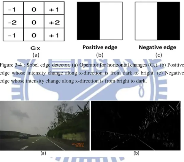
Figure 3-4 : Sobel edge detector. (a) Operator for horizontal changes (Gx). (b) Positive edge whose intensity change along x-direction is from dark to bright. (c) Negative edge whose intensity change along x-direction is from bright to dark. ... 24

Figure 3-5 : An example of edge detection result. (a) Original image. (b) Result of edge pixels which have positive responses after using Gx. ... 24

Figure 3-6 : Flowchart of Vanishing Point Computation and ROI Setting module. .... 25

Figure 3-7 : Result of Otsu binarization. (a) Original edge image. (b) The corresponding binary image after using Otsu algorithm. ... 27

Figure 3-8 : Hough transformation. (a) Polar-coordinate (ρ, θ) representation of a straight line. Each line has a unique representation (ρ, θ). (b) The Hough domain of an image. The red point is the point with the highest number of intersections [38]... 28

Figure 3-9 : The unreasonable representation of the curve lane lines. (a)(b) The curve lane lines in the red circle cannot be detected, and only the straight lane lines in the near field are detected. ... 29

Figure 3-10 : The estimated vanishing point result. (a) Original image. (b) The green lines are represented as the prominent lines acquired from the Hough transformation and the red point is represented as the estimated vanishing point in current frame. ... 31

Figure 3-11 : Procedure of vanishing point computation. From Nvan frames, choosing the highest voted point as the final result of the vanishing point which is drawn in yellow. ... 32

Figure 3-12 : Illustration of ROI setting. The yellow point indicates the final vanishing point, and the five rows (Nrow = 5) in red, green, cyan, yellow, and purple are the selected ROIs. ... 33

Figure 3-13 : Flowchart of Lane Line Detection and Verification module. ... 34

Figure 3-14 : Illustration of time slice generation. ... 35 Figure 3-15 : An example of temporal blurring. (a) Original image. (b) Average image.

(11)

ix

... 36 Figure 3-16 : The gradient histogram of each ROI shown with different colors. ... 37 Figure 3-17 : The result of gradient value adjustment. (a) Original gradient histogram of each ROI which sometime does not include the information of dashed lane line. (b) The gradient value adjustment algorithm compensates the detection of dashed lane line. The red cycle shows the final result of dashed lane line. ... 38 Figure 3-18 : The hill and peak point (Pp) in the histogram [41]. ... 39

Figure 3-19 : The result of gradient value smoothing. (a) Original gradient histogram with many internal ripples. (b) The gradient histogram only with the maximal peak after gradient value smoothing. ... 39 Figure 3-20 : The result of peak finding algorithm. Found (picked) peak points, represented by the white points. ... 40 Figure 3-21 : An example of peak connecting algorithm. (a) 5 peak points (blue) and the vanishing point (red). (b) Peak connecting result of (a). Each blue line segment means that two peak points are similar. ... 42 Figure 3-22 : The result of peak connecting on the real road image. (a) Peak point image. (The peak points are represented by the white points.) (b) Peak connecting image. (The white line segments imply the relationship within the similar peak points.) ... 42 Figure 3-23 : The result of candidate lane line detection. (a) Peak connecting image. (b) Two candidate lane lines are obtained in current frame (yellow lines). ... 43 Figure 3-24 : The result of lane line verification. (a) Two candidate lane lines are drawn with yellow color. (b) Final results of lane lines are drawn with cyan color. ... 44 Figure 3-25 : Elimination of the false candidate lane lines in lane line verification. (a) Original image. (b) Two false candidate lane lines are generated since the presence of arrow markings on the road. (c) Within M frames, these two false candidate lane lines are not detected consecutively and thus be eliminated. ... 44 Figure 3-26 : The relationship between the candidate list and tracking list. ... 45 Figure 3-27 : The conception of prediction procedure. (a) Two candidate lane lines are drawn with yellow color. (b) The time-slice image generated by ROI5 is

used to track the lane lines. (c) An example of the moving change over

x-axis. Here, x3 is the current point, and x4 is the predicted point. ... 46

Figure 4-1 : Sample road images in different cases. (a) Intermediate case where the type of lane lines is from the straight to the curve then back to straight. (b)

(12)

x

Lane changing case from left to right. (c) Straight lane lines case. ... 48 Figure 4-2 : The results of pre-processing step in [36]. (a) Original image. (b) Image after top-hat transformation. (c) Image after contrast enhancement. ... 50 Figure 4-3 : The result after the top-hat transformation and contrast enhancement. (a) Original image. (b) Image after top-hat transformation and contrast enhancement where the red cycle shows the destroyed part of the lane line. ... 51 Figure 4-4 : The result of line-structure constraint. (a) Original image. (b) Image after top-hat transformation and contrast enhancement. (c) Image after the line-structure constraint on (b). The red cycle shows the effectiveness of noise removal. ... 52 Figure 4-5 : A new lane line appears in the middle of two originally detected lane lines.

(a) Original images. (b) Output images... 52 Figure 4-6 : The intermediate case of driving from straight lane lines to curve lane lines then back to straight lane lines. (a) Original images. (b) Output images. ... 53 Figure 4-7 : The lane changing case. (a) Original images. (b) Output images. ... 53 Figure 4-8 : The straight lane line case. (a) Original images. (b) Output images. ... 53 Figure 4-9 : Problem 1 caused by the smoothing step. (a) Original images. (b) Output image where the left lane line is incorrect at the frame 465. ... 55 Figure 4-10 : The results under the different times of the smoothing step. (a) After 1 time of smoothing step, our system generates an incorrect lane line because of too many peaks in the gradient histogram. (b) After 4 times of smoothing step, the result of lane line detection is almost correct because of the proper gradient histogram. ... 55 Figure 4-11 : Problem 2 caused by the noises. (a) Noise from the leading vehicle. (b) Noise from the words. (c) Noise from the reflection of the windshield. 56

(13)

xi

List of Tables

Table 1 : The 1-D convolution kernel of Gaussian Filter [37]. ... 40

Table 2 : Total number of frames of each ground-truth video clip. ... 48

Table 3 : Processing time of each module in our system. ... 49

(14)

1

Chapter 1. Introduction

1.1 Motivation and Overview

Recently, traffic accidents have become one of the most serious problems in today’s world. However, the major factor which leads to road accidents is the carelessness of drivers or improper driving. Therefore, Advance Driver Assistance System (ADAS) [1] and Intelligent Transportation System (ITS) [2] are developed to improve the driving safety and reduce road accidents.

For the vision-based driving assistant systems, lane line detection plays an essential role in providing useful and effective information with respect to the relative position of the vehicle on the road. By means of this information, the driver can better understand the road circumstances and his/her driving situations for safety. So for decades, lane line detection has become a critical research field. However, in most conditions, vision-based lane line detection is simplified into a problem of finding the locations of lane lines in the input road images with or without strong prior knowledge about the lane line positions and drawing the results in the output images. Figure 1-1 shows an example of the lane line detection.

In order to analyze the lane line information from car videos, most lane line detection algorithms are based on image processing techniques to search for the lane lines. In general, the video analysis procedure comprises three major processing steps: (1) selection of the region of interest, (2) lane line detection, and (3) lane line tracking. Nevertheless, in most of the existing works, a fundamental problem is that the performance of video analysis may not be stable with varied environments and different weather conditions, as shown in Figure 1-2, resulting in the difficulty in lane

(15)

2

line detection. Besides, as shown in Figure 1-3, the presence of shadows, the lane line occluded by the vehicles and various markings on the road also affect the detection result. Moreover, most existing works processed the case of straight lane lines and curve lane lines, individually. Few researches discuss about the intermediate case of driving from the straight lane lines to curve lane lines, as shown in Figure 1-4, or lane changing, as shown in Figure 1-5. On the other hand, another critical issue is that image processing is always time-consuming. To cater for the requirement of real-time response, developing efficient system frameworks and video analysis algorithms is an important and inevitable task. Consequently, how to quickly and correctly locate the position of the lane lines from car videos is the core problem and issue in our work.

Figure 1-1 : An example of the lane line detection. (a) Input frame captured from the camera. (b) Output frame where the position of the lane lines is located.

Figure 1-2 : Different weather conditions. (a) Image captured under the sunny day. (b) Image captured under the cloudy day. (c) Image captured under the rainy day.

(16)

3

Figure 1-3 : Different driving environments. (a) The presence of shadows. (b) The lane line occluded by the vehicles. (c) Various markings on the road.

Figure 1-4 : An example of the intermediate case of driving from the (a) straight lane lines to (b) curve lane lines and then back to (c) straight lane lines.

Figure 1-5 : An example of lane changing from the left to right.

In this thesis, we describe our lane line detection and tracking system, then implement and compare several methods on the various cases, as shown in Figure 1-4 and Figure 1-5, and we discuss some problems arising in the course of our experiments. We mount the camera on the upper center of windshield of the vehicle for video capturing when driving. When inputting a car video, our proposed system

(17)

4

locates the vanishing point at first, and then instead of using the whole image, we only process some rows of the image as our rows of interest (ROIs). Slicing through the stack of some frames in time at a ROI generates a time slice image. With the time slice images and the vanishing point’s position, we can detect the lane lines and track them on the time slice images. In the experiment, we implement several lane line detection algorithms and test them on real car videos captured at special environment conditions, then we discuss the problems arising in the experiment.

In conclusion, the contributions of this thesis are listed as follows:

 We adopt the peak finding algorithm to find out the points of the candidate lane lines, instead of giving a fixed threshold to classify the pixels in the image into non-lane-line and lane-line classes.

 We propose a gradient value adjustment algorithm to overcome the sparseness problem in detecting dashed lane lines.

 We propose a lane line detection and tracking algorithm using the “time slice images” which involve the lane lines’ relationship between the time and space. Also, the time slice images can help us to detect the shape of curve lane lines without calculating the parameters of curve fitting.

1.2 Organization

The rest of this thesis is organized as follows. In Chapter 2, we survey some related works in lane line detection and tracking of car videos. Chapter 3 introduces our system to detect and track the position of lane lines. In Chapter 4, the experimental results of lane line detection and tracking are shown and discussed. At last, we conclude this thesis and describe the future work in Chapter 5.

(18)

5

Chapter 2. Related Works

In this chapter, some related works in lane line detection and tracking of car video are described. A distinction can be made between the problems of lane line detection and tracking. Lane line detection involves determining the location of the lane lines in a single image. Lane line tracking involves determining the location of the lane lines in a sequence of consecutive images, using information about the lane line location from previous images in the sequence to constrain the probable lane line detection in the current image. In each video, the first several image frames will be processed by the lane line detection algorithm, and this will provide a good estimation of lane line tracking for the subsequent frames.

2.1 Related Works in Lane Line Detection

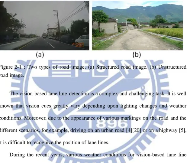
As a basic yet important component in driver assistance systems [1][3], the aim of lane line detection is to detect the relative position of the vehicle on the road and to obtain the lane line information, such as the offset, the orientation, the curvature, and the types. With this lane line information, we can provide a better understanding of road environment to drivers and thus improve the driving safety. Generally, a road image can be classified into a structured or unstructured one, as shown in Figure 2-1(a) and (b), respectively. The most distinguishable characteristic between structured roads and unstructured roads is the existence of lane lines. The structured road has its boundary showing specific features or certain regularity in appearance. The structured road boundary has characteristics such as the painted white or yellow line(s), and regularly

(19)

6

shaped road edges. On the other hand, the boundary of the unstructured road does not have apparent features or regularity in its appearance. Most researches of lane line detection focus on the analysis of structured roads where the lane lines are painted on the road surface.

Figure 2-1 : Two types of road image. (a) Structured road image. (b) Unstructured road image.

The vision-based lane line detection is a complex and challenging task. It is well known that vision cues greatly vary depending upon lighting changes and weather conditions. Moreover, due to the appearance of various markings on the road and the different scenarios, for example, driving on an urban road [4][20] or on a highway [5], it is difficult to recognize the position of lane lines.

During the recent years, various weather conditions for vision-based lane line detection techniques for safety vehicles are taken into consideration and are being developed. There have been many approaches proposed for lane line detection. Those works usually use different road models, 2D [7][12] or 3D [4][6][15][17][19]. Different lane lines, straight [12][14][15][28] or curve [10][30][33], and different lane line patterns, solid or dash painted line [3]-[30], are considered. Different techniques are employed, Hough transformation [11][28], template matching [10][25], or neural networks [8]. The recent survey paper proposed by McCall and Trivedi [3] provides a

(20)

7

comprehensive summary of existing approaches. Most of the methods propose a three-step process. (1) Initializing lane lines by extracting features such as edges [7], texture [8], color [9], and frequency domain features [10]. (2) Post-processing the extracted features to remove outliers using techniques like Hough transform [11][28] and dynamic programming [12], along with computational models explaining the structure of the road using deformable contours [13], and regions with piecewise constant curvatures [6]. (3) Tracking the detected lane lines using the Kalman filter [14] or particle filter [15][16] by assuming motion models such as constant velocity or acceleration for the vehicle. However, these approaches can be classified into two main categories namely feature-based and model-based techniques [3]. Detailed surveys can be found in [3]-[30].

2.1.1 Feature-based Lane Detection

The feature-based methods detect the lane lines in the road images by using some low-level features, such as painted lines [17]-[19], lane line edges [7][22][23], texture [8] and colors [9][20][21]. The advantage of the feature-based methods is that the features are extracted easily. Nevertheless, they highly demand well-painted lane lines or strong lane line edges in road images; otherwise this method may fail. Furthermore, the performance of this method may easily suffer from occlusion or noise. In the following, we review some representative works of feature-based lane line detection.

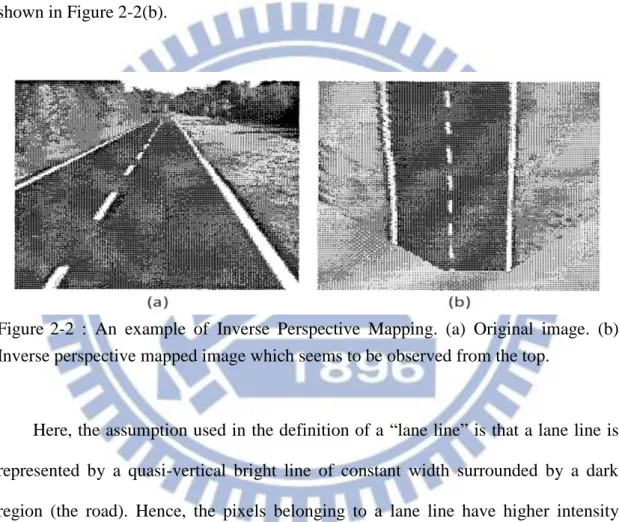
Broggi and Bertè [17][18] develop an approach applying the IPM (Inverse Perspective Mapping) [42] algorithm on the road image. The IPM algorithm is a mathematical technique whereby a coordinate system may be transformed from one perspective to another, and it can remove the perspective effect from the acquired image. The perspective effect means that the lane lines width change according to

(21)

8

their distance from the camera. In this case, in order to remove the perspective effect, the a-priori knowledge exploited by the IPM transform is the assumption of a flat road in front of the vehicle. The IPM algorithm maps the acquired image, as shown in Figure 2-2(a), into a new 2-D domain array in which the information content is homogeneously distributed among all pixels and the resulting image represents a top view of the road region in front of the vehicle, as if it were observed from the top, as shown in Figure 2-2(b).

Figure 2-2 : An example of Inverse Perspective Mapping. (a) Original image. (b) Inverse perspective mapped image which seems to be observed from the top.

Here, the assumption used in the definition of a “lane line” is that a lane line is represented by a quasi-vertical bright line of constant width surrounded by a dark region (the road). Hence, the pixels belonging to a lane line have higher intensity values than their left and right neighbors. Thus, the lane line detection is reduced to the determination of horizontal black-white-black transitions. Based on a geometrical transform and on a fast morphological processing, the system is capable of detecting the lane lines. Figure 2-3 shows the results of lane line detection through the IPM algorithm.

(22)

9

Figure 2-3 : Lane line detection through the removal of the perspective effect in three different conditions: straight road with shadows, curved road with shadows, junction. (a) Input image. (b) Mapped image (3D to 2D) of (a). (c) Result of the line-wise detection of black-white-black transitions in the horizontal direction. (d) Remapped image (2D to 3D) where the grey areas represent the portion of the image shown in (c). (e) Superimposition of (d) onto a brighter version of the original image (a). [18]

Bertozzi and Broggi [19] propose the GOLD (Generic Obstacle and Lane Detection) system utilizing a stereo vision-based hardware and software architecture, which aims at improving road safety of moving vehicles. The GOLD system removes the perspective effect also by IPM algorithm which maps the region ahead of the vehicle into the top view. In GOLD, lane lines after the IPM transform are modeled as quasi-vertical constant width lines, brighter than their surrounding region. Based on a line-wise determination of horizontal black-white-black transitions, the pixels that have higher intensity value than their horizontal neighbors at a given distance are

(23)

10

detected. However, in this work, not only the lane line detection is implemented but also the obstacle detection.

He et al. [20] propose a color-based vision system to determine the road parameters and detect lane lines from urban traffic scenes. Based on the projective transformation, edge detection, binarization and their pre-defined curvature models, as shown in Figure 2-4, this system estimates three candidate boundaries to extract the road region. The result of boundary estimation module is combined with the color information of the capture image to get the road area image. Finally, they utilize this road area image and three candidate boundaries to determine the real road boundaries and to acquire the parameters of road. Cheng et al. [21] apply the color of road and lane lines for the image segmentation, and then utilize the size, shape and motion characteristics to determine whether a region belongs to a vehicle or a lane line for false lane line region elimination. Huang and Pan [22] develop a method to detect the lane lines and the road edges of structured and unstructured roads, respectively. In structured road detection, utilizing the vertical Sobel mask and color characteristic at first to detect the points of lane lines. If the number of points is greater than a predefined threshold, the slope filtering is applied to refine the detection results. And the least square approximation is employed to represent the lane lines. The unstructured road detection is performed while the number of detected points is not enough. They extract the road surface with the predefined sets of sampled blocks, and obtain the edge points from the vertical intervals. For the accuracy of detection, the new sampled blocks are updated by the random sampling points from segmented regions.

(24)

11

Figure 2-4 : The flowchart of He et al.[20]. (Red rectangle is represented as the curvature model they defined.)

Tsai et al. [23] propose a lane line detection algorithm using the concept of directional random walks based on Markov process. Two major components are included in this method to decide the correct locations of all lane lines: (1) lane segmentation and (2) edge linking. They first define proper structure elements to extract different lane line features from input frames using a novel morphology-based approach. Then, they utilize a novel linking technique to link all “desired” lane line features for lane lines detection. The technique considers the linking process as a directional random walk which constructs a Markov probability matrix for measuring the direction relationships between lane segments. Then, from the matrix of transition probability, the correct locations of all lane lines can be decided and found in videos. Yim and Oh [24] develop a three-feature based automatic lane line detection algorithm

(25)

12

(TFALDA). It is intended for automatic extraction of the lane lines without the priori information or manual initialization under different road environments. The lane lines are recognized based on similarity match in a three dimensional (3D) space consisting of the starting position, direction, and gray-level value of a lane line as features, as shown in Figure 2-5.

Figure 2-5 : The lane line candidate vectors mapped into the 3D feature space.

2.1.2 Model-based Lane Detection

Model-based methods represent the lane lines through a few geometric parameters. According to the shapes of lane lines, the lane line models can be defined as a straight line model [12][14][15][28] or a parabolic model (that is, curve) [10][30], even a spline model [4][13][29]. Moreover, how to find the best parameters for the model is the core problem to be solved. Compared with the feature-based methods, the model-based methods are less sensitive to weak lane line appearance features and noise.

To acquire the best parameters of lane line model, the likelihood function [10][25], the Hough transform [11][28], and curve fitting [30], had been applied into the lane line detection. However, the model-based methods require a complex modeling process involving much prior knowledge. Constructing a simple model for

(26)

13

one scene can get better efficiency, but this model may not work well in another scene because it cannot describe arbitrary shape of lane lines. So, the simple models are less adaptive. But for the complex models, although they can adapt to multiple scenes and describe arbitrary shape of lane lines, an iterative error minimization algorithm should be applied for the estimation of best model parameters, which is comparatively time-consuming. The process would take much time and would not satisfy the real time requirement of the driving applications. Next, we discuss some representative works of model-based lane line detection.

In [25], Kluge and Lakshmanan present a deformable template model of lane line structure, called Likelihood Of Image Shape (LOIS), to locate the lane lines by optimizing a likelihood function. It is assumed that the left and right lane lines are modeled as two parallel parabolas on the flat ground plane. For each pixel, this algorithm uses a Canny edge detector [26] to obtain the gradient magnitude and orientation. The parameters of perspective projection model are then estimated by applying the Maximum A Posteriori (MAP) estimation [27] and the Metropolis algorithm based on the image gradient. Figure 2-6 shows some results of LOIS’ lane detection under the various road environmental conditions.

(27)

14

The LANA system [10], proposed by Kreucher and Lakshmanan, is similar to the LOIS system [25] at the detection stage. But LANA combines the frequency domain features of the lane lines with a deformable template for finding the lane line edges. The feature vectors are used to compute the likelihood probability through fitting the detected features to a lane line model. Li et al. [11] develop the Springrobot system by using the color and edge gradient as the lane line features and the adaptive randomized Hough transform (ARHT) to locate the curve lane lines on the feature map. A multi-resolution strategy is applied to achieve an accurate solution rapidly and to decrease the running time to meet the real-time requirement. As illustrated in Figure 2-7, they first reduce the size of the original image to 1/2z, where z = 1, 2, by bicubic interpolation. The reduced images are called “half image” and “quarter image”, respectively. In these images with lower resolution, they apply the ARHT with fixed quantized accuracy to roughly and efficiently locate the global optima of lane lines without regarding the accuracy. The parameters resulting from the previous step can be used as starting values of another ARHT for more accurate location of lane lines. Therefore, the parameter search can be restricted to a small area around the previous solution, saving time and storage complexities. This coarse-to-fine location speeds up the process of lane line detection, thus it offers an acceptable solution at an affordable computational cost. Figure 2-7 shows the results of multi-resolution algorithm in Springrobot system.

(28)

15

Figure 2-7 : Multiresolution algorithm for detecting the lane line rapidly and accurately [11], which uses the size reducing at first, then applies the ARHT to detect the parameters of lane lines roughly, and finally uses coarse-to-fine location method to offer the better position of lane lines.

Park et al. [30] use the lane-curve function (LCF) for lane line detection. The whole process of algorithm is shown in Figure 2-8. The LCF is obtained by transforming the defined parabolic function from the world coordinates into the image coordinates. Moreover, this algorithm needs no transformation of the image pixels into the world coordinates. The main idea of this algorithm is to search for the best-described LCF of the lane-curve on an image. In advance, several LCFs are assumed by changing the curvature and for each LCF, it defines its lane line region of interest. Then, the comparison is carried out between the slope of an assumed LCF and the phase angle of the edge pixels in the lane line region of interest. The LCF with the minimal difference in the comparison becomes the true LCF corresponding to the lane-curve.

(29)

16

Figure 2-8 : The process overview of LCF [30].

Wang et al. [29] propose a Catmull-Rom spline [32] based lane line model. Their algorithm uses a maximum likelihood approach in detecting the lane lines. As Catmull-Rom spline model can form arbitrary shapes by control points, it can describe a wider range of lane line structures than the straight or parabolic model. Figure 2-9 shows the estimation of lane lines to real road image by implementing the Catmull-Rom spline algorithm. In [13], Wang et al. propose a B-Snake based lane line detection and tracking algorithm without any camera parameters. The main characteristics of this method are as follows. (1) The Canny/Hough Estimation of Vanishing Point (CHEVP) is presented for providing a good initial position for the B-Snake. (2) The Minimum Mean-Square Error (MMSE) is proposed to determine the control points of the B-Snake model by the overall image forces on two sides of the

(30)

17

lane. (3) The Gradient Vector Flow (GVF) [31] field is used to let the B-Snake move to its optimal solution. The estimation of lane lines by B-Snake is shown in Figure 2-10.

Figure 2-9 : An example of lane line detection by Catmull-Rom spline. (a) Original road image. (b) The result of lane line detection by Catmull-Rom splines. ( PL0, PL1,

PL2) and ( PR0, PR1, PR2) are the control points for left and right side of lane line. PL0

and PR0 are the same control point, which supposes to be vanishing point. [29]

Figure 2-10 : Examples of lane line detection using the B-Snake. [13]

2.2 Related Works in Lane Tracking

However, some researches [7][8][10][12][20][23][30] do not mention about the idea of lane line tracking. They only propose the lane line detection algorithm on each

(31)

18

single frame and do not take into consideration about the relationship between two consecutive frames. However, most researches [6][9][14][15][16][21][28] usually include the lane line tracking into their systems for the purpose of the real-time requirement. Hence, considering there is only small change between two consecutive frames, those systems use information from previous results to facilitate the current detection. The Kalman filter [14] or the Particle filter [15][16] is the common method used to track the lane lines in videos since it can provide the continuous detection on all images in a sequence. Lane line tracking step can drastically reduce the search area in every frame and consequently detect lane lines in an efficient way.

In [14], when the lane lines are detected, the Kalman filters are used to track and smooth the estimates of parameters of lane lines based on the measurements. While tracking, if lane lines are intermittently not detected, then the Kalman filter relies on its prediction to produce estimates. However, if the lane lines go undetected for more than a few seconds, then tracking is disabled until the next detection. This is to avoid producing incorrect estimates when the lane lines do not appear on the road.

Kim [16] choose a particle-filtering algorithm over the Kalman filter to prevent the result from being biased too much on the predicted vehicle motion but to give more weight to the image evidence. Due to the vehicle’s vibration and pitch change, the motion of the lane lines in world coordinates is not smooth enough to be properly modeled by a Kalman filter.

Although a lot of lane line detection and tracking algorithms are proposed, few researches mention about the intermediate case of driving from the straight lane lines to the curve lane lines, or the lane changing case. Therefore, we implement several algorithms in the intermediate case and the lane changing case. Then we discuss the problems arising in the experiments.

(32)

19

Chapter 3. Proposed System Architecture

This chapter describes the details of our proposed system. At first, an overview is given in Section 3.1, and the pre-processing is described in Section 3.2. Section 3.3 introduces the method to compute the vanishing point and set the row of interest (ROI) for subsequent processing steps. Then our proposed approach of lane line detection and verification is presented in Section 3.4, and finally, we explain the lane line tracking algorithm in Section 3.5.

(33)

20

3.1 Overview of the Proposed System

The overview of proposed system is depicted in Figure 3-1. The system architecture consists of four modules, including (1) Pre-processing, (2) Vanishing

Point Computation and Row of Interest (ROI) Setting, (3) Lane Line Detection and Verification, and (4) Lane Line Tracking. For each step, we show the sample results on

the right side.

For each image acquired from the camera, Pre-processing step for noise removal is firstly performed by image smoothing, image normalization and edge detection. In

Vanishing Point Computation and Row of Interest (ROI) Setting step, the Hough

transform and linear least square are applied in order to decide the possible position of the vanishing point and then utilize the vanishing point to delimit the rows of interest (ROIs) which we want to analyze in the following steps. Next, Lane Line Detection

and Verification uses the gradient histogram of edge image generated from edge

detection and some limitations to obtain the lane lines. Lastly, Lane Line tracking tracks the lane lines on the time-slice images generated from the ROIs.

3.2 Pre-processing

In this section, pre-processing is performed to reduce the noise and improve the contrast of the original image, then generate the corresponding edge image for subsequent processing. As illustrated in Figure 3-2, the original color image is first converted to the grayscale image. For image smoothing, we use the Gussian filter to eliminate the noise. Then in order to facilitate the extraction of lane lines, we use image normalization to increase the contrast of the image. At last, we extract the edge

(34)

21

features of the lane lines by edge detection.

Figure 3-2 : Flowchart of Pre-processing module.

3.2.1 RGB to Gray

At the beginning, the original images are composed of three independent channels for red, green and blue primary color components. Thus, for RGB to grayscale

(35)

22

conversion, we take three channel values of each pixel in the color image and use the conversion formula defined by Eq. (1) [37] to get the value for the corresponding pixel in the grayscale image. Pixels throughout the RGB image are scanned and this procedure is applied to convert a RGB image into grayscale one.

Gray = 0.299 * Red + 0.587 * Green + 0.114 * Blue

(1)

3.2.2 Image Smoothing

To realize the lane line detection, noise disturbance can greatly affect lane line distinction. However, the noise reduction techniques usually involve averaging the value of pixels residing in a local area and generating a blurred or smoothed image. Here, we apply the Gaussian filter [37] to eliminate the noise signal. As one of the specialized weighted averaging filters, the Gaussian filter has been widely adopted in the field of image processing and computer vision for years, and is known for its image smoothing and noise reduction capability.

3.2.3 Image Normalization

Since there are different environment conditions such as the presence of strong shadows, object reflection, illumination variation, and obscurity, the contrast enhancement of image intensity is essential. Image normalization [37] is a spatial domain based image enhancement technique. After image normalization, the distribution of pixels becomes more evenly spread out over the available pixel range. This step normalizes the brightness values of image in the range from 0 to 255, ensuring that the lane lines have high intensity value in every frame, even when the

(36)

23

overall brightness is changing. Figure 3-3 shows an example of image normalization.

Figure 3-3 : An example of image normalization. Comparing the original histogram of image after smoothing (top) with the normalized histogram of image after normalization (bottom), one can observe that the range of pixel intensity values becomes broader.

3.2.4 Edge Detection

After smoothing and normalizing the image, we want to utilize some features to recognize the lane lines. In order to attract the drivers’ attentions, a lane line is usually painted in a special color and owns high contrast (or high edge responses) to the neighboring road surface. Since color features are easily affected by light changes and become unclear at night, we tend to detect the lane lines based on the edge feature and

acquire the edge information by Sobel edge detector. Since the horizontal gradient of the lane line is visible, the 3x3 operator for horizontal changes (Gx) is used, as shown

(37)

24

values of edge pixels are obtained. However, as shown in Figure 3-4(b) and (c), Sobel edge detector usually generates the positive and negative edges at the rim of the object. For computation efficiency, here we only retain the positive edge in the image. Figure 3-5 shows an example of the edge detection result.

Figure 3-4 : Sobel edge detector. (a) Operator for horizontal changes (Gx). (b) Positive

edge whose intensity change along x-direction is from dark to bright. (c) Negative edge whose intensity change along x-direction is from bright to dark.

Figure 3-5 : An example of edge detection result. (a) Original image. (b) Result of edge pixels which have positive responses after using Gx.

3.3 Vanishing Point Computation and ROI Setting

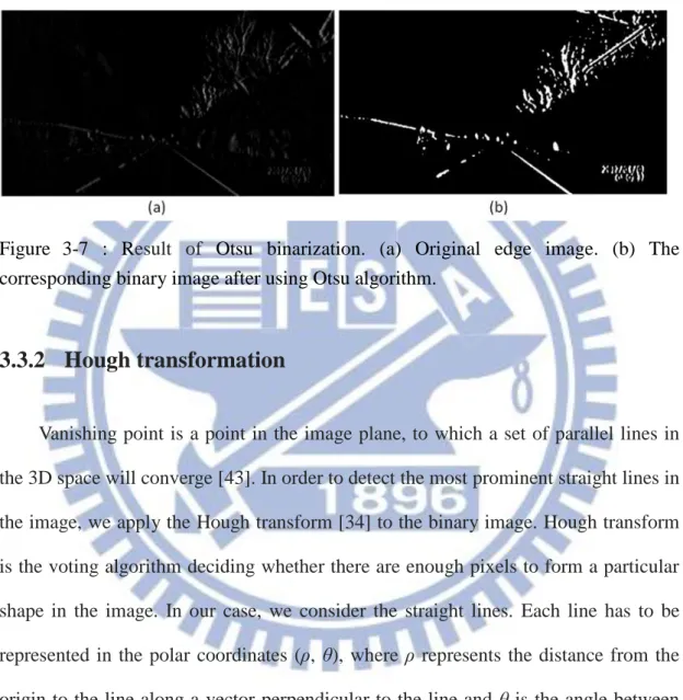
In this section, we intend to locate the vanishing point and set the row of interest (ROI) according to vanishing point. As illustrated in Figure 3-6, we first use the Otsu

(38)

25

algorithm to binarize the edge image and then the Hough transformation is applied to extract the representative lines. For each frame, we use the linear least square to estimate the position of the vanishing point from those representative lines. After processing serveral frames, we can locate the position of vanishing point with highest probability. As soon as we get the vanishing point, the ROIs are also defined. The details of the module are described as follows.

(39)

26

3.3.1 Otsu Binarization

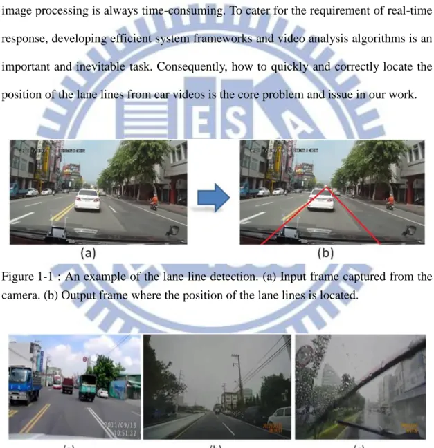
For the reason that the Hough transformation only accepts a binary image as input, thresholding is utilized here to segment the edge image. Nevertheless, as the lighting conditions are different, an adaptive threshold should be used in this stage. Otsu algorithm [33] is used to search for an ideal threshold adaptively.

The Otsu method exhaustively searches for the threshold which minimizes the intra-class variance, defined as a weighted sum of variances of the two classes. The thresholding process can be simplified into a process about how to partition the image pixels into two classes: C1 = {0, 1, …, T} and C2 = {T+1, T+2, …, Ngl -1}, where Ci

indicates class, T is the chosen threshold and Ngl is the number of gradient levels of

the image. The intra-class variance σ 2intra-class is defined as

)

(

)

(

)

(

)

(

)

(

₁ ₁2 ₂ ₂2 2 class intra

T

q

T



T

q

T



T



_





(2)

where qi(T) and σ i2(T) indicates the proportion and gradient variance of the Ci pixels,

respectively. The class probabilities are estimated as Eq. (3), the means of class are given by Eq. (4), and the individual class variances are defined as Eqs. (5) and (6).

(

)

(

)

(

)

(

)

1 2 1 1

T

H

i

and

q

T

H

i

q

gl N T i T i



  



₍₃₎



  



gl N T i T i

q

T

i

iH

T

and

T

q

i

iH

T

1 2 2 1 1 1

)

(

)

(

)

(

)

(

)

(

)

(



₍₄₎









T i

q

T

i

H

T

i

T

1 1 2 1 2 1

)

(

)

(

)]

(

[

)

(





₍₅₎



 





gl N T i

q

T

i

H

T

i

T

1 2 2 2 2 2

)

(

)

(

)]

(

[

)

(





₍₆₎

(40)

27

When the threshold T is chosen, the effect of edge image segmentation is obtained through reserving the edge pixels whose gradient levels exceed T. Figure 3-7

shows the result of Otsu algorithm.

Figure 3-7 : Result of Otsu binarization. (a) Original edge image. (b) The corresponding binary image after using Otsu algorithm.

3.3.2 Hough transformation

Vanishing point is a point in the image plane, to which a set of parallel lines in the 3D space will converge [43]. In order to detect the most prominent straight lines in the image, we apply the Hough transform [34] to the binary image. Hough transform is the voting algorithm deciding whether there are enough pixels to form a particular shape in the image. In our case, we consider the straight lines. Each line has to be represented in the polar coordinates (ρ, θ), where ρ represents the distance from the origin to the line along a vector perpendicular to the line and θ is the angle between the x-axis and the vector perpendicular to the line, as shown in Figure 3-8(a), so that a generic point (x, y) belonging to a line will satisfy the following equation:

xcos(θ) + ysin(θ) = ρ (7)

Therefore, by means of Hough transform, a line can be represented as a single point in the polar-coordinate parameter space. Similarly, since infinite lines pass

(41)

28

through any given pixel in the original image, the representation of a pixel in the parameter space is a unique sinusoidal curve (representing all the lines that can pass through that pixel). However, the point of intersection between multiple sinusoidal curves in the parameter space means the line passing through multiple pixels. In the other words, the more cumulative number of the intersection points, the more pixels a line passes through. As illustrated in Figure 3-8(b), the red point represents the line which passes through P1 and P2. The parameter space is divided into bins in the ρ and

θ space. The total number of intersections in each bin is saved into the accumulator,

and then the highest voted lines are returned. Here, in order to save the computation time, we only consider the top 5 lines in the accumulator.

In fact, most related works apply the Hough transformation to detect the lane lines [28][36], and show good performance of the results on the straight lane lines in the road images. However, the Hough transform-based methods can only detect the straight lane lines in the image and the case of driving on the curve lane lines cannot be handled well, as shown in Figure 3-9.

Figure 3-8 : Hough transformation. (a) Polar-coordinate (ρ, θ) representation of a straight line. Each line has a unique representation (ρ, θ). (b) The Hough domain of an image. The red point is the point with the highest number of intersections [38].

(42)

29

Figure 3-9 : The unreasonable representation of the curve lane lines. (a)(b) The curve lane lines in the red circle cannot be detected, and only the straight lane lines in the near field are detected.

There are other types of Hough transformation to recognize the shapes like circles and ellipses that are mathematically expressed in a binary digital image. When the parameters of the circles or ellipses are known in advance, the Hough transformation works well. Otherwise, it is difficult to recognize the curves without prior-knowledge. In addition, some works [6][10][14][16][25][30] utilize the curve fitting to detect the curves. Suppose each point (x, y) belonging to a curve will satisfy the following equation:

2 3

2

1

x

s

x

s

y





(8) where sj (j = 1, 2, 3) are the parameters of the curve. Then the idea of the curve fitting

is to find the best parameters sj (j = 1, 2, 3) which minimize E and E is defined as:

2 3 2 2 1 1

)]

(

[

y

s

x

s

x

s

E

_i _i _i k i









 (9)

where k is the total number of pixels used to fit a curve. This method is intuitive, but we have to know which pixels belong to the curve before curve fitting method. It is the limitation of this method. In addition, the more the number of detected pixels we use in curve fitting, the more time used in calculating the parameters we need.

(43)

30

curve lane lines efficiently. We exploit the time-slice image inspired by [14] to detect and track the lane lines. Hence, we need to compute the position of the vanishing point at first.

3.3.3 Vanishing Point Computation

After acquiring several prominent lines in the image by Hough transformation, we use the “Linear Least Square” [40] to estimate the position of vanishing point in each frame. Our method is similar to the Vanishing Point Detection method in [44]. Now we have a linear system which involves several linear equations and several variables. A general system of m linear equations with n unknowns can be written as:

m n mn n n m m n n

b

u

a

u

a

u

a

u

a

u

a

u

a

b

u

a

u

a

u

a









2 2 2 2 2 22 1 1 1 21 1 1 2 12 1 11









(10)

where ui (i = 1, 2, …, n) are the unknowns, ai (i = 11, 12, …, mn) are the coefficients

of the system, and bi (i = 1, 2, …, m) are the constant terms. A solution of the linear

system is an assignment of values to ui (i = 1, 2, …, n) that satisfies all m equations

simultaneously. In matrix-vector notation, the linear system is represented as

AU



B

(11) where

,

2 1 2 22 21 1 12 11















mn m m n n

a

A







and

2 1















n

u

U

















m

b

B



2 1 (12)

In our case, each linear equation determines a line on the xy-plane, so the n is equal to two. Next, we solve this linear system AU=B with Singular Value Decomposition (SVD) [39] to obtain the closest possible solution U. This is

(44)

31

equivalent to minimize the squared norm ∥AU-B∥2, which is a linear least square optimization problem. Figure 3-10 shows the estimated vanishing point result (the red point) in current frame.

Figure 3-10 : The estimated vanishing point result. (a) Original image. (b) The green lines are represented as the prominent lines acquired from the Hough transformation and the red point is represented as the estimated vanishing point in current frame.

However, the vanishing point cannot be detected well in some frames. Hence, how to determine the best and correct vanishing point becomes the issue for us to conquer currently. We consider that the position of vanishing point should not move drastically during a car video, so we add the time conception to choose the correct vanishing point.

Observing Nvan frames, we record all detected vanishing points and apply the

voting method by an accumulator, whose concept is similar to the Hough transformation, to all vanishing points. When the Euclidean distance between two vanishing points is less than a pre-defined threshold, those two vanishing points are treated as the same point, and then their vote is incremented by 1. The highest voted point represents the correct vanishing point we want. The procedure of vanishing point computation is shown in Figure 3-11.

(45)

32

Figure 3-11 : Procedure of vanishing point computation. From Nvan frames, choosing the highest voted point as the final result of the vanishing point which is drawn in yellow.

3.3.4 ROI Setting

Once the position of vanishing point is obtained, we delimit the rows of interest (ROIs) which are the main parts we want to process within the whole image. Generally, the road region appears under the vanishing point. Under this condition, our ROIs are selected from the region Rregion under the vanishing point in the image.

Nevertheless, instead of processing whole region Rregion, we only take evenly Nrow

rows within the bottom three-quarter part of Rregion as our ROIs. The illustration of

(46)

33

Figure 3-12 : Illustration of ROI setting. The yellow point indicates the final vanishing point, and the five rows (Nrow = 5) in red, green, cyan, yellow, and purple are the

selected ROIs.

3.4 Lane Detection and Verification

In this section, we detect the candidate lane lines and then a verification procedure is performed to remove the false ones. As illustrated in Figure 3-13, we first generate the time-slice image for each ROI to record the moving of lane lines. Then we adjust the edge gradient histogram of each ROI when a new frame comes for enhancing the detection of dashed lane lines. Next, using the smoothing method and peak finding algorithm on the gradient histogram to obtain the peak points. With these peak points, we utilize some constraints to connect the similar peak points together, and further detect the candidate lane lines. Generally, the lateral shift of the vahicle is small between two consecutive frames, that is, the difference of the lane line positions is small between two consecutive frames. Therefore, we can detect the lane line positions in current frame from the surrounding area of the lane line position in the last frame. At last, we verify the candidate lane lines by the concept similar to tracking. The details of this module are described in the following sections.

(47)

34

Figure 3-13 : Flowchart of Lane Line Detection and Verification module.

3.4.1 Time-Slice Image Generation

Inspired by [14], time-slice image generation greatly assists in the detection and tracking of lane lines, especially when the vehicle runs from the straight lane lines to

(48)

35

curve lane lines or the condition of changing lane happens, which are still challenging tasks for state-of-the-art works. Supposing that a video sequence totally have F frames, and each frame fi (i = 1, …, F) is a WH image. Then we record the specific

row Rrow of pixels from each frame in time, and thus we generate a WF time-slice

image, as shown in Figure 3-14. Besides, the index of each row of time-slice image is

f, which means the frame number.

Figure 3-14 : Illustration of time slice generation.

3.4.2 Gradient Value Adjustment

Due to the discontinuousness of the dashed lane lines, detecting dashed lane lines in a single image becomes difficult and Hough transformation based lane line detection technique cannot work well. In order to overcome this obstacle, Borkar et al. [14] propose the temporal blurring algorithm, which adds the time conception to

(49)

36

generate an average image, giving the dashed lane lines the appearance of a near continuous line by connecting them. The concept of temporal blurring is to take only a few frames from the past in the averaging. The average image is defined as follows:



   past 0 past ) ( ge AverageIma N i N i n I (13)

where I is the intensity of current frame, n is the index of current frame, and Npast is

the number of frame from the past. Hence, the detection of these dashed lane lines becomes easier since they appear as a connected lines in the image. An example of temporal blurring is shown in Figure 3-15.

Figure 3-15 : An example of temporal blurring. (a) Original image. (b) Average image.

The temporal blurring algorithm is a good method to facilitate the detection of dashed lane lines. It is an important issue to determine how many frames should be used for in the averaging process. If too many frames are used, the perceived width of the lane lines will be altered; otherwise, if we use only a few frames, the effect of temporal blurring will become unobvious. In brief, this method is dependent on the moving speed of the vehicle. In our work, a method capable of detecting the dashed lane lines without considering the vehicle speed is proposed.

(50)

37

is recorded. Figure 3-16 shows the gradient histogram of each ROI in the image with different colors. However, due to the discontinuousness of dashed lane lines, not every ROIs can get the gradient information of lane lines in current frame. As shown in Figure 3-16, the gradient value of the left dashed lane line is only recorded on the first and third ROIs. For resolving this obstacle, we propose the gradient value adjustment algorithm to retain the lane line information. The detail of this algorithm is described in Algorithm 1. For each ROI, we first set an accumulative gradient histogram to record the change of value. Then, for each pixel, we compare its gradient value in current frame with the value of corresponding pixel in accumulative histogram. If the current value is less than the accumulative value, we will decrease the accumulative value by one. This method can avoid decreasing the value too fast to retain the position of the dashed lane line. Otherwise, if the current value is larger than the accumulative value, the current value will substitute for the accumulative value. Afterward, repeating the above steps until all ROIs are examined. We also need

Npast frames from the past to obtain the completed information of dashed lane lines.

However, the advantage of our algorithm is that we do not have to give Npast in

advance, Npast is automatically determined in the process. (Npast = 3 in our experiment

averagely.) The result of gradient value adjustment is illustrated in Figure 3-17.

(51)

38

Algorithm 1: Gradient Value Adjustment

Input: The accumulative gradient value of each ROI (h) and the gradient value of each ROI in current frame (g) Output: The gradient value of each ROI after adjusting

1 for each ROI do

2 for j = 0 to width //each pixel on the ROI 3 if (gj < hj) then hj = hj -1; 4 if (hj < 0) then hj = 0; 5 endif 6 endif 7 else hj = gj; 8 end for 9 end for

Figure 3-17 : The result of gradient value adjustment. (a) Original gradient histogram of each ROI which sometime does not include the information of dashed lane line. (b) The gradient value adjustment algorithm compensates the detection of dashed lane line. The red cycle shows the final result of dashed lane line.

3.4.3 Gradient Value Smoothing

As shown in Figure 3-17, there are several “hills” in the gradient histogram of each ROI. A formal definition of the “hill” [41] can be given as: A range over which the values increase first and decrease next without any internal ripples in the histogram. As illustrated in Figure 3-18, the peak point (Pp) is the point which has

車輛影片中車道線之偵測及追蹤

國

立

交

通

大

學

資訊科學與工程研究所

碩

士

論

文