適用於動態無線近身網路媒體存取控制層的通道模型

國立交通大學

電子工程學系電子研究所碩士班

碩 士 論 文

適用於動態無線近身網路媒體存取控制層

的通道模型

A MAC Channel Model for Dynamic Wireless Body Area

Networks

研 究 生 : 蔡志強

指導教授 : 黃經堯 博士

適用於動態無線近身網路媒體存取控制層的通道模型

A MAC Channel Model for Dynamic Wireless Body Area Networks

研 究 生 : 蔡志強 Student : JhihCiang Cai

指導教授 : 黃經堯 Advisor : Ching-Yao Huang

國 立 交 通 大 學

電 子 工 程 學 系 電 子 研 究 所 碩 士 班

碩 士 論 文

A Thesis

Submitted to Department of Electronics Engineering & Institute of Electronics College of Electrical and Computer Engineering

National Chiao Tung University In partial Fulfillment of the Requirements

For the Degree of Master of Science

In

Electronics Engineering

July 2009

HsinChu, Taiwan, Republic of China

I

適用於動態無線近身網路媒體存取控制層的通道模型

學生 : 蔡志強 指導教授 : 黃經堯博士

國立交通大學電子工程學系電子研究所碩士班

摘要

無線近身網路(WBAN)近來年在醫療照顧以及醫學應用上受到重視。在這深具 潛力的無線網路系統領域中，目前已經有許多通道模型被提出。然而，這些被提 出的通道模型大部分都是以物理層的角度來提出的，且當中鮮少是以動態的量測 為基礎。 在本論文中，我們提出了一個專為媒體控制層所設計的動態通道模型。我們 量測兩個重要的行為，步行與睡眠。除了考量所接收訊號振幅的統計特性之外， 我們另外也研究這二種行為各自在時間上的相關性來強化在媒體控制層的模型 準確度。我們提出了雙階層模型以及三層次模型來分別特性化這兩種行為。藉由 在模型中考量時間的相關性，所提出的模型可以在媒體存取層達到相當高的模型 準確性。

II

A MAC Channel Model for Dynamic Wireless

Body Area Networks

Student : JhihCiang Cai

Advisor : Dr. Ching-Yao Huang

Depart of Electronics Engineering

Institute of Electronics

National Chiao Tung University

Abstract

Wireless body area network (WBAN) has been paid attention in health-care and medical application field in recent years. Many of the channel models have been proposed for this potential wireless network system. However, most of them are built in physical layer, and they seldom analyze the body channel in dynamic scenario.

In this thesis, we propose a MAC channel model for dynamic WBAN. We perform the dynamic measurement of two vital behaviors, walking and sleeping. Apart from considering the conventional statistics of received power amplitude, the model also investigates the time-domain correlation of those two activities to enhance the modeling accuracy in MAC. We propose the two-state model and three-level model to characterize the two behaviors, respectively. With the consideration of time-domain correlation in modeling, the proposed models can achieve high accuracy with the measured data in MAC point of view.

III

誌

謝

碩士班的時光匆匆，在新竹兩年的求學生涯也將告一段落。在這碩士班的兩 年之中，首先誠摯的感謝指導教授黃經堯老師的悉心教導使我得以一窺無線通訊 領域的深奧，不時的討論並指點我正確的方向，使我在這些年中獲益匪淺。老師 對學問的嚴謹更是我學習的典範。 兩年裡的日子，實驗室裡共同的生活點滴，學術上的討論、趕作業的革命情 感，有你們的陪伴讓兩年的研究生活變得多彩多姿。 首先，感謝士恒、子宗、 冠穎、理銓、純孝、志展、宗耿與東佑學長們不厭其煩的指出我研究中的缺失， 且總能在我迷惘時為我解惑。 此外，要感謝我同屆的好夥伴們易達、禹伸、信 駿與明憲，與你們共同度過的時光是我最美的回憶。實驗室學弟妹們裕華、英昌 美玲、美齡、怡萱與傳佑當然也不能忘記，你們的幫忙與陪伴我銘感在心。 再來，要感謝我的女朋友宜君在背後的默默支持更是我前進的動力。最後， 我要感謝我最愛的家人，爸爸、媽媽、哥哥及良美阿姨。當我遇到瓶頸與困難時， 你們總是提供我最大的溫暖、給予我無止境的包容與鼓勵， 在此，謹以我的畢業論文獻給大家，希望你們能分享我的成果與喜悅，感謝 你們。 蔡志強 謹誌 2009 年 7 月

IV

Contents

中文摘要 ... I Abstract ... II 誌 謝 ... III Contents ...IV List of Tables ...VI List of Figures ... VII

Chapter 1 Introduction ... 1

Chapter 2 Overview of Wireless Body Area Network ... 3

Chapter 3 Relative works ... 6

3.1 On-body channel model ... 6

3.2 On-body to off-body channel model ... 8

Chapter 4 Measurement Setup ... 10

Chapter 5 Proposed dynamic WBAN channel model ... 13

5.1 Goals ... 13

5.2 Two-State WBAN walking channel model ... 14

5.2.1 RSSI measurement results – Walking ... 14

5.2.2 Construct the WABN Walking channel model ... 16

5.2.2.1 Analysis of the parameters in Two-state walking model ... 17

5.2.2.2 Conclusion of building a Two-state Walking Model ... 20

5.3 Three-level WBAN Sleeping channel model ... 23

5.3.1 construct a Three-Level Sleeping model ... 25

5.3.1.1 Duration of each state 𝐓𝐧 ... 25

5.3.1.2 Mean and standard deviation of each state ... 26

5.3.2 Conclusion of building a Three-Level Sleeping model ... 28

Chapter 6 Simulation Setup ... 30

6.1 Path Loss data ... 30

V

Chapter 7 Simulation Results ... 33

7.1 Simulation of two-state walking channel model... 33

7.1.1 UDP Analysis ... 33

7.1.1.1 Throughput... 33

7.1.1.2 Delay Difference ... 35

7.1.1.3 Discussion of UDP analysis ... 36

7.1.2 TCP Analysis ... 37

7.1.2.1 Throughput... 37

7.1.2.2 Delay Difference ... 38

7.1.2.3 Discussion of TCP Analysis ... 39

7.2 Simulation of Three-level Sleeping channel model ... 40

7.2.1 UDP Analysis ... 40

7.2.1.1 Throughput... 40

7.2.1.2 Delay Difference ... 42

7.2.1.3 Discussion of UDP analysis ... 43

7.2.2 TCP Analysis ... 44

7.2.2.1 Throughput... 44

7.2.2.2 Delay Difference ... 45

7.2.2.3 Discussion of TCP analysis ... 46

Chapter 8 Conclusion and Future Work ... 47

8.1 Conclusion ... 47

8.2 Future Work ... 48

VI

List of Tables

Table 5-1 Parameter of Two-state walking model ... 22

Table 5-2 Parameters of Three-level sleeping model ... 29

Table 6-1 Environment setting in NS3 simulation ... 32

Table 7-1 Statistic of throughput in UDP analysis - Walking model ... 34

Table 7-2 Statistic and packet error rate of delay difference in UDP analysis - Walking model ... 36

Table 7-3 Statistic of throughput in TCP analysis - Walking model ... 38

Table 7-4 Statistic of delay difference in TCP analysis - Walking model ... 39

Table 7-5 Statistic of throughput in UDP analysis - Sleeping model ... 41

Table 7-6 Statistic and packet error rate of delay difference in UDP analysis - Sleeping model ... 43

Table 7-7 Statistic of throughput in TCP analysis - Sleeping model ... 45

VII

List of Figures

Figure 2-1 Process of WBAN automatic medical service [12] ... 3

Figure 2-2 Wireless body area networks (WBAN) ... 4

Figure 4-1 CC2500 RF Transceiver from Texas Instrument ... 10

Figure 4-2 Timeline of the data acquisition cycle at the receiver in sleeping scenario ... 11

Figure 4-3 Antenna locations on test subject ... 11

Figure 4-4 Layout of the indoor condition ... 12

Figure 5-1 Tx: Right wrist / Rx: Right Hip, Walking, 180 seconds RSSI measurement ... 14

Figure 5-2 Gamma distribution. Best fit for Tx: Right wrist / Rx: Right Hip, Walking ... 15

Figure 5-3 Part of the walking experiment result (60s to 80s) ... 16

Figure 5-4 The power spectrum density of Walking Received power amplitude ... 17

Figure 5-6 Distribution of the Upper-state and Lower-state power(mw) ... 18

Figure 5-7 Distribution of the 𝐓𝐩𝐞𝐫𝐢𝐨𝐝 (second) ... 19

Figure 5-8 Distribution of the 𝐓𝐫𝐚𝐭𝐢𝐨𝐧𝐇𝐋 ... 20

Figure 5-9 On-body(chest) to Off-body, Sleeping, 4.8Hours RSSI measurement ... 23

Figure 5-10 Concept of Sleeping channel model ... 24

Figure 5-11 Distribution of the duration 𝐓𝐧 ... 25

Figure 5-12 Power spectrum density of the duration 𝐓𝐧 ... 25

Figure 5-13 Proposed Three-level sleeping channel model ... 27

Figure 5-14 RSSI(dbm)-PSR(%), 4.8hours Sleeping measurement ... 27

Figure 6-1 Path loss of walking model ... 31

VIII

Figure 7-1 Throughput in UDP analysis - Walking model ... 33

Figure 7-2 Distribution of throughput in UDP analysis - Walking model ... 34

Figure 7-3 Delay difference in UDP analysis - Walking model ... 35

Figure 7-4 Distribution of delay difference in TCP analysis - Walking mode ... 35

Figure 7-5 Throughput in TCP analysis - Walking model ... 37

Figure 7-6 Distribution of throughput in TCP analysis - Walking model ... 37

Figure 7-7 Delay difference in TCP analysis - Walking model ... 38

Figure 7-8 Distribution of delay difference in TCP analysis - Walking model ... 39

Figure 7-9 Throughput in UDP analysis - Sleeping model ... 40

Figure 7-10 Distribution of throughput in UDP analysis - Sleeping model ... 41

Figure 7-11 Delay difference in UDP analysis - Sleeping model ... 42

Figure 7-12 Distribution of delay difference in UDP analysis - Sleeping model ... 42

Figure 7-13 Throughput in UDP analysis - Sleeping model ... 44

Figure 7-14 Distribution of Throughput in TCP analysis - Sleeping model ... 44

Figure 7-15 Delay difference in TCP analysis - Sleeping model ... 45

1

Chapter 1

Introduction

Wireless body area network (WBAN) has been paid attention in health-care and medical field in recent years. One of the most promising applications is the wireless patient monitoring. The prototypes of the health-care WBAN like HUMAN++ [1] and WiBoC [2] have already been promoted. By wireless medical monitoring, medical service will be ubiquitous, and patient is no longer constrained in his location and activity. For instance, medical WBAN can continuously monitor the important vital signals like ECG, blood pressure, temperature and SPO2 which can be reported to remote medical unit for further diagnosis. In other words, WBAN could be responsible for the “last meter” transmission in the ubiquitous health care system. Therefore, providing a high reliable WBAN system becomes a very important issue. Channel modeling is seen as the first step to develop a communication system, learning the knowledge of WBAN channel model become quite important.

A number of channel models for WBAN have been proposed [3]-[9]. But most of them build the channel model in physical layer, and they seldom analyze the body channel in dynamic scenario. Nation ICT Australia (NICTA) has presented a dynamic human on-body and on-body to off-body WBAN channel model [7]-[9], which characterized the measured received signal amplitude with well-known statistical model. However, it is lack of modeling accuracy as we consider the end to end latency and queuing condition which is in MAC point of view. For this reason, in this thesis, we proposed a Two-state walking channel model, which consider the time domain correlation in channel model to improve the modeling accuracy in MAC layer. Besides, we also proposed the Three-level sleeping channel model to model the channel conditions of sleeping behavior. The simulation in NS3 demonstrate our two

2

types of channel model can better reflect the channel characteristic in MAC point of view, as we compare the end to end delay difference and throughput results with the measured data.

The rest of this thesis is organized as follows: In chapter 2, the overview of Wireless Body Area Network. In chapter 3, the relative works of WBAN channel model. Chapter 4 gives a description of the experimental setup of this thesis. In chapter 5, the proposed dynamic WBAN channel model will be discussed detailed. In chapter 6, the setting of simulation platform is addressed. In chapter 7 shows the simulation result. Finally in chapter 8, the conclusion and future work will be provided.

3

Chapter 2

Overview of Wireless Body Area Network

IEEE 802.15 working group established a study group in recent years, body area network (SG-BAN), to develop guideline for using wireless technologies for medical device communications in various healthcare services [10]. The main argument for wireless is an enabled to provide people more comfortable and convenient use environment, and supply better access and greater physical mobility. By wireless medical monitoring, patient is no longer constrained in his movements. WBAN can be used to offer the automatic medical service through monitoring of living body signal. There is a wide range of potential applications and user scenarios in hospital, home and gym. The typical application scenarios of WBAN system include the ward monitoring in a hospital, the home healthcare and emergency diagnosis for the chronic, elder and child. Figure 2-1 shows the automatic medical service and its process. Necessary medical data is collected from the living body by wireless sensors (wireless sensor nodes) and send to the near receiver (central processing node), and then the receiver upload this data to the hospital. A doctor or a nurse who accept data can make a decision based on received patient's conditions.

4

Figure 2-2 Wireless body area networks (WBAN) (a) Topology of WBAN (b) Traffic load of WBAN

The architecture of WBAN consists of two classes of devices: Central Processing Node (CPN) and Wireless Sensor Node (WSN), as shown in Figure 2-2(a). [11]. The WSNs continuously monitor the vital signals and transmit them to the CPN, and then the CPN pass them to the remote medical unit like hospital or clinic, etc.As shown in Figure 2-2(b), WBAN is a simple star topology, it could have many WSNs but only one CPN. In the star topology, CPN plays the role of a master and WSNs are the slaves. CPN has the central control of the join, leave of WSNs, and it also do the slot assignment to avoid collision in data transmission. CPN will be embedded in personal devices like mobile phone, notebook, PDA, etc. Due to the bandwidth limit of current wireless network service, CPN can’t transmit the entire collected vital signals to the remote medical unit. Therefore, the CPN should judge the data before transmit it. Users can modify the CPN settings according to individual requirements or target diseases. When CPN sense the received physiological signals as unusual, it will simultaneously alert the user and deliver the anomalous signals to the remote medical station to do the immediately diagnose. On the contrary, WSNs are passive

5

devices. WSNs are designed for retrieving specific vital signals like temperature, blood pressure, ECG, etc and send to CPN based on pre-regulated transmission policies. A user combines different WSNs for the monitoring of target symptom.

In addition to the applications of WABN, “Changing fast” is another key characteristic of WBAN. The channel conditions between CPN and WSNs change just because the human take walk in the park, swing his arms, or even turn their body when they are sleeping. The simple motions we do everyday can sometimes heavily alter the link quality of WBAN. It’s serious as we focus on the health-care application of WBAN. Therefore, getting the knowledge of channel characteristic of some vital behaviors like walking and sleeping become quite important, because it can help us to have the strategy to conquer those problems and to design a high reliable WBAN system.

6

Chapter 3

Relative works

As mentioned before, many of Wireless Body area channel models have been presented. Most of them focus on static channel characteristics. However, in this chapter, we introduce some researches about dynamic WBAN channel model which measure the body channel in motion. Firstly, we describe the on-body WBAN channel model which is relative to our walking channel model [7]-[8]. Secondly, we describe the on-body to off-body channel model, which is correlative to proposed on-body to off-body sleeping channel model [9]. Both of them are presented by Nation ICT Australia (NICTA).

3.1 On-body channel model

A statistical characterization of on-body WBAN channel model has been presented by [7]-[8]. In this work, some well-known statistical models are used to characterize on-body channel with different Tx-Rx pair locations such as “right wrist to right hip”, ”left wrist to right hip”, etc for subject’s standing, walking and running.

The following are the statistic models they try to fit dynamic WBAN channel and its probability density function, respectively:

 Normal is well known for their maximum entropy characteristics. Channels which have no significant structure are well modeled by these distributions.

𝑓 𝑥|𝜇, 𝜎 = 1

σ 2πexp

− 𝑥 − 𝜇 2

7

 Lognormal distribution arises from a law-of-large numbers approach to multiplicative effects, and is commonly used to model shadowing in terms of the average power received.

where ln(.) represents the natural logarithm.

 Gamma distribution is used in model mobile fading channels.

where Γ(.) denotes the Gamma function.

 Weibull has been used for multipath modeling and is generally found to model small-scale fading and multipath inter-arrival processes well.

In this research it concludes that the characteristic of dynamic on-body channel with different Tx-Rx locations can be well described by statistic models. In some cases like “right wrist to right hip” walking scenario the Gamma and Weibull distributions provide good fit to the normalized amplitude distribution according to their maximum-likelihood (ML) estimates. However in general the Lognormal distribution provides best fit to the received signal statistics, particularly with the subject moving while either running or walking. However, according to this conclusion, we analyze the delay difference and throughput in NS3. The simulation

𝑓 𝑥|𝜇, 𝜎 = 1 xσ 2πexp − 𝑙𝑛 𝑥 − 𝜇 2 2𝜎2

(2)

𝑓 𝑥|𝑎, 𝑏 = 1 ba_{Γ 𝑎} xa−1exp 𝑥 𝑏

(3)

𝑓 𝑥|𝑎, 𝑏 = 𝑓 𝑥 = −𝑏𝑎−𝑎𝑥𝑏−1exp − 𝑥 𝑎𝑏 , 𝑥 ≥ 0 0 , 𝑒𝑙𝑠𝑒

(4)

8

results show that pure statistical walking model is scanty in modeling accuracy. For this reason, in this thesis, we are going to present a two-state model which reflects the regularity and repeatability of walking behavior for human body to improve the

shortage of existent models.

3.2 On-body to off-body channel model

The On-body to off-body channel characterization is present by NICTA [9]. In This work, it presents a number of channel measurements conducted with a transmitting antenna located on the body of a test subject and another receiving antenna located or the body some distance away. The transmitting antenna is worn on either the chest or the right wrist with measurements taken while the test subject:

1. perform two different actions (standing still or walking on the spot). 2. face in four different directions (0°, 90°, 180° and 270°) with 0° representing

the subject facing the receive antenna and 90°representing the subject facing 90° to the right of the receive antenna.

3. stand either 1, 2, 3 or 4 meters away from the receive antenna.

In this study of transmission on the human body to off the body in an indoor environment, it concludes:

1). Movement of the human body is the dominant fading effect which cause the time-selective fading. However, as human body standing still there is clearly observable frequency-selective fading which is caused by multipath effect in the indoor environment.

9

than the path loss around the human body documented in [8] even in the smaller on-body transmitter and off receiver distance.

3). The Lognormal distribution is the best matching model to data sets of normalized received power for on-body to off-body communications while the subject is in motion.

4). Normal distribution provides the best fit in some cases of the human standing still with on-body to off-body measurement.

From this research, we can get the information of the statistical characteristic of on-body to on off-body measurement with different directions and distant. It’s useful as we consider the sleeping behavior which people often turn their body to different directions in one night. However, it’s not enough as we try to build a practical sleeping channel model which still needs to consider the time domain correlation in sleeping model. For this reason, in chapter 5 we will present the three-level sleeping model which considers the time domain correlation in model.

10

Chapter 4

Measurement Setup

In this chapter, we introduce the experimental setup in this thesis. Wireless on-body and on-body to off-body channel measurements are made using cc2500 RF transceiver from Texas Instrument as shown in figure 4-1 and tape to the body of a 165 cm / 63 kg male test subject in both outdoor (walking in the campus) and indoor (sleeping) environment, respectively.

(a).Transmitter (b).Receiver

Figure 4-1 CC2500 RF Transceiver from Texas Instrument

Channel measurements are performed by transmitting test signals centered in regions around the 2400 MHz ISM bands. The test signals are continuously transmitted from one antenna while the subject is in two different scenarios: 1) walking in the campus; 2) sleeping on the bed. The signal is received at the other antenna and saved to SD card. Duo to the limit of the transmission device, the minimum sampling duration is 27ms, and it is also the sampling rate (37Hz) we set in the walking experiment. Besides, as shown in figure 4-2, for the purpose to simulate the real WBAN sensor transmission interval, we set one second break between each continuous 20 packets transmission cycle for the transmitter. By the 20 transmitted

11

packets in each cycle, we can calculate the average received RSSI value and success rate in each acquisition cycle.

Figure 4-2 Timeline of the data acquisition cycle at the receiver in sleeping scenario

The transmission Power is set to 0dbm and -12dbm in walking and sleeping measurement, respectively. For those two experimental scenarios, the transmitting and receiving antennas were placed on different locations. Figure 4-3,4-4 illustrate the locations of both the Transmitter and receiver in walking and sleep measurement, respectively. In walking experiment, transmitter is placed on right wrist, and the receiver is on right hip. On the other hand, in the sleeping scenario, the transmitter and receiver is separated 50cm from each other, Tx placed on chest of the body with Rx placed on the table near the bed. The total experimental duration is 180 seconds and 4.8 hours for the walking and sleeping RSSI measurement respectively.

Figure 4-3 Antenna locations on test subject

1.3 second break

: Tx : Rx Back of the body

12

Figure 4-4 Layout of the indoor condition

5m

5m

cabinet

Toilet

Rx

Table

Tx

Bed

13

Chapter 5

Proposed dynamic WBAN channel model

Just as mentioned before, channel model is seen as the first step to develop a reliable WBAN system. Therefore, in this chapter, we will propose a two-state WABN walking channel in section 5.2 and a three-level sleeping channel model in section 5.3, and the RSSI measurement results will also be shown in each section respectively. And in chapter 6 and 7 will introduce the simulation setup and show the simulation results.

5.1 Goals

Our goal is to propose a dynamic channel model which is in MAC point of view. As we said before, channel modeling is seen as the first step to develop a communication system. However, most of the proposed WBAN channel models focus on building the channel model in physical layer, and they seldom analyze the body channel in dynamic scenario. Although the researches of NICTA give us some knowledge of dynamic channel model, it still can’t reflect the queue conditions in MAC which need to consider the time domain correlation. For this reason, we have to build a channel model which includes the time correlation to improve the scarcity of NICTA’s model. Besides, sleep is a vital behavior of each person, it almost occupies a third of time. However, there is no channel model designed for this important scenario. So, in this chapter, we are going to characterize this important behavior. And for the purpose to simplify the construction of our model, we analyse the RSSI value instead of SNR. Both of the two proposed models must truly reflect the queuing state to achieve the requirement of modeling accuracy in MAC.

14

5.2 Two-State WBAN walking channel model

Following show the RSSI measurement results of test subject walking in the campus. The Transmitter and Receiver were taped to the right wrist and right hip of the test subject, respectively.

5.2.1 RSSI measurement results – Walking

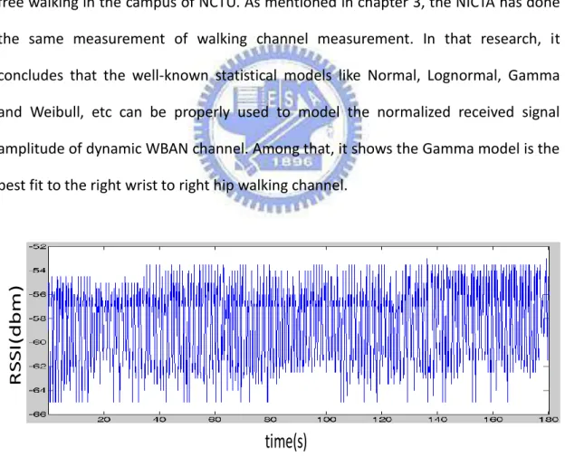
Figure 5-1 shows the total 180 seconds RSSI measurement result of test subject free walking in the campus of NCTU. As mentioned in chapter 3, the NICTA has done the same measurement of walking channel measurement. In that research, it concludes that the well-known statistical models like Normal, Lognormal, Gamma and Weibull, etc can be properly used to model the normalized received signal amplitude of dynamic WBAN channel. Among that, it shows the Gamma model is the best fit to the right wrist to right hip walking channel.

Figure 5-1 Tx: Right wrist / Rx: Right Hip, Walking, 180 seconds RSSI measurement

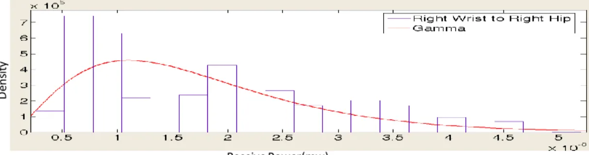
The figure 5-2 shows our measurement result is equal to the conclusion of NICTA, which Gamma is the best fit. The received power (mw) of Gamma walking model can

time(s)

R S S I( dbm )

15

be obtain from (3) with a and b is equal to 2.7600 and 6.2606e-007, respectively. In order to compare between the four models we mentioned in before, in this thesis we use the Akaike information criterion (AIC) [13], as chosen in [14] for wideband characterization, to choose the best fitting model for our channel model. The second order AIC (AICc) is given by:

𝐴𝐼𝐶𝑐 = −2 loge(𝑙(𝜃 |𝑑𝑎𝑡𝑎)) + 2𝐾 +

2𝐾(𝐾 + 1)

(𝑛 − 𝐾 − 1) (5)

where loge(𝑙(𝜃 |𝑑𝑎𝑡𝑎)) is the value of the maximized log likelihood over the

unknown parameters (𝜃), given the data and the model, K is the number of parameters estimated in the model and 𝑛 is the sample size. This equation is straightforward to compute since the log likelihood is readily available from the ML estimates. Intuitively, the first term indicates that better models have a lower because the log-likelihood reflects the overall fit of the model to the data. The second part of the equation penalizes additional parameters ensuring we select models that best fits the data with the least number of parameters.

Figure 5-2 Gamma distribution. Best fit for Tx: Right wrist / Rx: Right Hip, Walking

D

en

si

ty

16

5.2.2 Construct the WABN Walking channel model

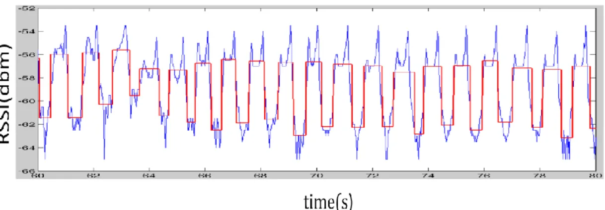
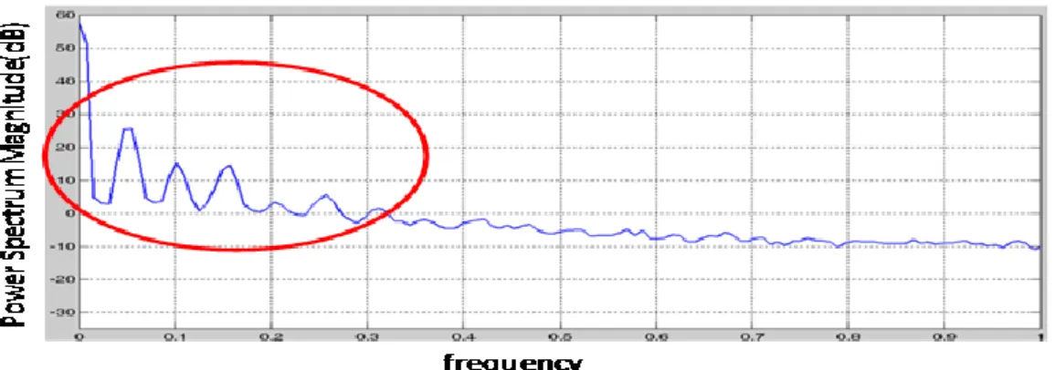
As shown in Figure 5-3, because of the regular movement of walking activity, the periodic RSSI variation can be simplified as two sates, upper-state and lower-state. In Figure 5-4 the power spectrum density of received power amplitude of walking motion shows there exist the dominate frequency in lower frequency part. It is because the walking channel condition changes along with the repetitive and regular movement of test subject like swing of arms and body movement during walking. It also means that if we apply this time domain correlation in our model, we can efficiently improve the modeling accuracy in MAC layer, which needs to put the queuing state into consideration. Therefore, the two-state walking channel model is presented in Figure 5-5. Our two-state walking model can be seen as two parts: 1) duration of each Upper-Lower period; 2) RSSI value of upper and lower-state. Due to the repetitive and regular characteristic of the RSSSI value, in our two-state model, we classify the RSSI into two states which replace the upper-state RSSI value and lower-state RSSI value respectively, and each of them holds a short duration.

17

Figure 5-4 The power spectrum density of Walking Received power amplitude

`

Figure 5-5 The proposed two-state walking model

5.2.2.1 Analysis of the parameters in Two-state walking model

In following article of this section, we will give a detailed introduction of our two-state walking model. In the analyses below, AIC is still the criterion we used to compare the four distribution models (Normal, Lognormal, Gamma and Weibull). All of the parameters we use to build our model are traced from the measured data that is the same as Figure 5-1. In our model, there are three important elements that we need to determine:

18

1.

𝑹𝑺𝑺𝑰𝑼𝒑𝒑𝒆𝒓𝑺𝒕𝒂𝒕𝒆 , 𝑹𝑺𝑺𝑰𝑳𝒐𝒘𝒆𝒓𝑺𝒕𝒂𝒕𝒆

In Our analysis of RSSIUpperState , RSSILowerState , firstly, we should transfer

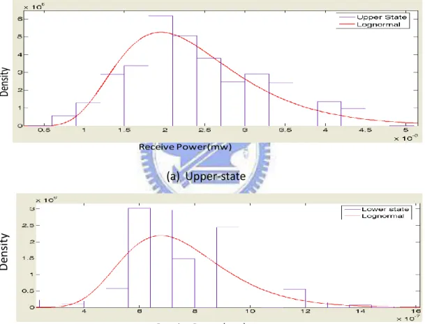
the RSSI which is in dBm to power(mw) to take the value within the range of each distribution (Lognormal, Gamma and Weibull). The Figure 5-6 shows the distribution of upper and lower state power value (mw). According to the AICc, the lognormal model provides the best fit to those two states.

(a) Upper-state

(b) Lower-state

Figure 5-6 Distribution of the Upper-state and Lower-state power(mw)

De ns ity Receive Power(mw) D ens ity Receive Power(mw)

19

2.

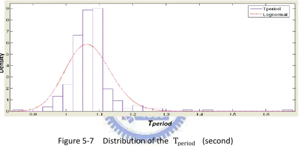
𝑻𝒑𝒆𝒓𝒊𝒐𝒅𝒏

The Tperiod is used to decide the duration of the whole walking procedure.

Where

𝑇𝑝𝑒𝑟𝑖𝑜 𝑑𝑛 = 𝑇𝑈𝑛 + 𝑇𝐿𝑛 , 𝑛 ∈ 𝑁 (6)

And the 𝑇𝑈𝑛 , 𝑇𝐿𝑛 replaced the duration each Upper-state and Lower-state.

In the Figure 5-7, it shows the Lognormal model is the best fit to the Tperiod

according to the AICc.

Figure 5-7 Distribution of the Tperiod (second)

3.

𝑻𝒓𝒂𝒕𝒊𝒐𝒏𝑯𝑳𝒏

The TrationH Lnis the ratio of the duration of Upper-state and Lower-state.

where

𝑇𝑟𝑎𝑡𝑖𝑜𝑛𝐻 𝐿𝑛 =

𝑇𝑈𝑛

𝑇_𝐿𝑛 , 𝑛 ∈ 𝑁 (7)

20 where 𝑇_𝐿𝑛 =𝑇𝑝𝑒𝑟𝑖𝑜𝑑𝑛 1 + 𝑇_{𝑟𝑎𝑡𝑖𝑜𝑈𝐿𝑛} , (8) 𝑇_𝑈𝑛 = 𝑇_{𝑝𝑒𝑟𝑖𝑜𝑑𝑛} − 𝑇_𝐿𝑛 , 𝑛 ∈ 𝑁 (9)

As shown in Figure 5-8, according to the AICc, the Lognormal model is also the best fit to the TrationH Ln.

Figure 5-8 Distribution of the TrationHL

The three elements above help us to decide the RSSI value of upper and lower state and the duration of each Upper-Lower period that we just mentioned before.

5.2.2.2 Conclusion of building a Two-state Walking Model

In this section, we give some functionsthat can help us to obtain 1) duration of each upper-lower period; and 2) RSSI value of upper and lower state; to build the

T ratioHL

De

ns

21

two-state model as shown in Figure 5-5. 1). Duration of each Upper-Lower period

As mentioned before, Lognormal distribution is the best fit to both Tperiod

and TratioUL , so we can obtain:

𝑇𝑝𝑒𝑟𝑖𝑜𝑑𝑛 = 𝑙𝑜𝑔𝑛𝑜𝑟𝑚𝑎𝑙 𝜇𝑡 𝑝𝑒𝑟𝑖𝑜𝑑, 𝜎𝑡 𝑝𝑒𝑟𝑖𝑜𝑑 , 𝑛 ∈ 𝑁 (10)

𝑇𝑟𝑎𝑡𝑖𝑜𝑈𝐿𝑛 = 𝑙𝑜𝑔𝑛𝑜𝑟𝑚𝑎𝑙 𝜇𝑡 𝑟𝑎𝑡 𝑖𝑜𝑈𝐿, 𝜎𝑡 𝑟𝑎𝑡𝑖𝑜𝑈𝐿 , 𝑛 ∈ 𝑁 (11)

And we can derive 𝑇_𝑈𝑛 and 𝑇_𝐿𝑛 from (8), (9).

2). RSSI value of Upper and Lower state

As mentioned before, the distribution of received power (mw) in both upper state and lower state is Lognormal, so we can obtain:

𝑃𝑜𝑤𝑒𝑟_𝑈𝑛 = 𝑙𝑜𝑔𝑛𝑜𝑟𝑚𝑎𝑙 𝜇_{𝑃𝑜𝑤𝑒𝑟𝑈}, 𝜎_{𝑃𝑜𝑤𝑒𝑟𝑈} , 𝑛 ∈ 𝑁 (12) 𝑃𝑜𝑤𝑒𝑟𝐿𝑛 = 𝑙𝑜𝑔𝑛𝑜𝑟𝑚𝑎𝑙 𝜇𝑃𝑜𝑤𝑒𝑟𝐿, 𝜎𝑃𝑜𝑤𝑒𝑟𝐿 , 𝑛 ∈ 𝑁 (13)

where the 𝑃𝑜𝑤𝑒𝑟𝑈 and 𝑃𝑜𝑤𝑒𝑟𝐿 are in mw, so the RSSI value can be

obtained in (14).

𝑅𝑆𝑆𝐼 𝑡 = 𝑅𝑆𝑆𝐼_{𝑅𝑆𝑆𝐼}𝑈𝑝𝑝𝑒𝑟 = 10 𝑙𝑜𝑔 𝑃𝑜𝑤𝑒𝑟𝑈 , 𝑡 ∈ 𝑇𝑈𝑛

𝑈𝑝𝑝𝑒𝑟 = 10 𝑙𝑜𝑔 𝑃𝑜𝑤𝑒𝑟𝐿 , 𝑡 ∈ 𝑇_𝐿𝑛 , 𝑛 ∈ 𝑁

(14) The Table 5-1 lists all the μ and σ above. The function of lognormal distribution is (2) in chapter 2. for x > 0, where μ and σ are the mean and standard deviation of the variable's natural logarithm (by definition, the variable's logarithm is normally distributed).

22

Table 5-1 Parameter of Two-state walking model

Data Lognormal Μ σ Tperiod (s) 0.064 0.063 TratioHL 0.415 0.212 PowerU (mW) -13.013 0.363 PowerL (mW) -14.136 0.259

23

5.3 Three-level WBAN Sleeping channel model

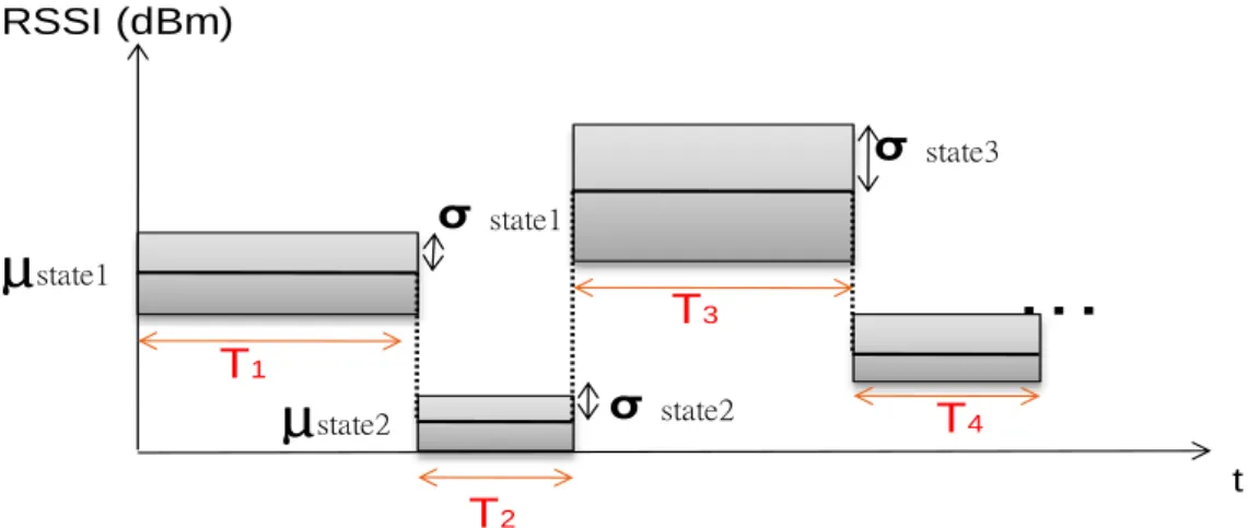
In this section, we give an introduction of how to build a WBAN sleeping model. The RSSI measurement of sleeping scenario is shown in Figure 5-9. In Figure 5-9, the red line represents the RSSI value we measured during the test subject is sleeping, and the black denotes the mean of RSSI in each short state. As we can see, the RSSI value performs like the stair that is composed of many short states, and each state of the stair holds a period of time. This is because when people is sleeping, it can be seen as a static scenario, the evidently change of RSSI caused by test subject turning his body, and the small variation is due to frequency-selective fading as subject is static (because there is not time-selective fading due to movement) [9]. This is the main idea in our sleeping model. Figure 5-10 shows the concept of the sleeping model. The conceptual sleeping model is consisted of two part of parameter: 1) duration of each state; 2) RSSI value of each state.

Figure 5-9 On-body(chest) to Off-body, Sleeping, 4.8Hours RSSI measurement

Time (s) RS S I( dBm )

24

Figure 5-10 Concept of Sleeping channel model

The duration of each state is represented by Tn in Figure 16. And the formula of

RSSI value is shown in (15).

RSSI t = Normal 0, σstaten2 + µstaten , t ∈ Tn , n ∈ N (15)

where µ_staten and σt_{state n} are the mean and standard deviation of each state. And

T_n is the duration of each state.

Tossing of the human body during sleeping causing time-selective fading is the dominant fading effect and is represented by µ_state. And the σstate is cause by

multi-path frequency-selective fading in indoor environment in the case of the subject is static. From (15), it is seen as if we obtain the knowledge of µ_state,

σstate and the duration T of each state we can build the dynamic sleeping channel

model. For this reason, in the following article of this section, we will focus on how to formulate those parameters.

T1 T2 T3 T4

…

RSSI (dBm) t

µ

state1

µ

state2 σ state1 σ state2 σ state3

25

5.3.1 construct a Three-Level Sleeping model

As mentioned before, the sleeping channel model is consisted of 1) duration of each state Tn; 2) RSSI value of each state. In this section we will give a detailed

introduction of those three elements.

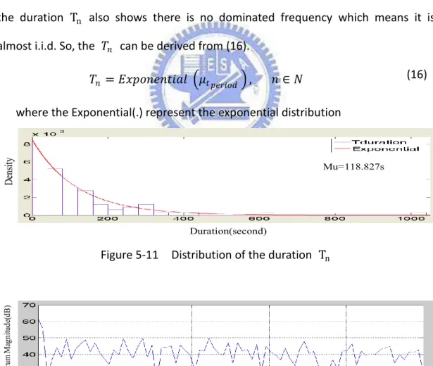
5.3.1.1 Duration of each state 𝐓

_𝐧

The duration of each state is characterized by exponential distribution according to AICc and is shown in figure 5-11. And in figure 5-12 the power spectrum density of the duration Tn also shows there is no dominated frequency which means it is

almost i.i.d. So, the 𝑇𝑛 can be derived from (16).

𝑇_𝑛 = 𝐸𝑥𝑝𝑜𝑛𝑒𝑛𝑡𝑖𝑎𝑙 𝜇_{𝑡 𝑝𝑒𝑟𝑖𝑜𝑑} , 𝑛 ∈ 𝑁 (16) where the Exponential(.) represent the exponential distribution

Figure 5-11 Distribution of the duration Tn

Figure 5-12 Power spectrum density of the duration Tn Mu=118.827s Duration(second) D ens ity frequency Po w er S pe ct ru m M ag ni tu de (d B )

26

5.3.1.2 Mean and standard deviation of each state

As we can see from the Figure 5-9, the RSSI of the conceptual sleeping model consisted of many states, and the mean and standard deviation of each state is different to each other. So, how do we simplify this circumstance to build our dynamic sleeping model?

Markov Chain can be use to resolve this multi-state condition. Firstly, we set the threshold of RSSI to classify the multi-state RSSI to fewer states. So, we need to know how many states can sufficiently reflect the channel condition in MAC. We have learned about that the MAC does the retransmission for the error packets. For this reason, we assume that the success rate of definite RSSI value higher than 50% can get the correct transmission during the retransmission procedure before the next data comes from the upper layer. Equally, the packet which success rate of definite RSSI is less than 50% will only have 50% to reach the highest throughput after retransmission. Besides, the packet which RSSI is too low to have only 0% success rate will no chance to get any correct transmission.

From the discussion above, we know that three-level model is enough for sleeping channel model in MAC. So, we simplify the RSSI value to three levels, high, medium and low-level, as shown Figure 5-13. The µ_{new −state}in Figure 5-13 is different to µ_state we just mentioned in Figure 5-10, and it denotes the new mean of each state in created three-level sleeping model. Figure 5-14 shows the measured RSSI to success rate plot of our 4.8hours sleeping scenario experiment. From this figure, we can obtain the high-threshold RSSI value, which success rate is equal to 50%. But, due to the scatter characteristic in our measured result which means one RSSI value would probably maps to more than one success rate, the RSSI of success rate equal to 50% is more than one value. Therefore, the high-threshold is calculated

27

as the mean of those RSSI values which success rate is equal to 50%. And we obtained the RSSI of high-threshold is equal to -63.785dbm.

Figure 5-13 Proposed Three-level sleeping channel model

Figure 5-14 RSSI(dbm)-PSR(%), 4.8hours Sleeping measurement

The low-threshold of our three-level sleeping model is set to the RSSI which success rate is equal to 0%, -65.5dbm, the lowest received power of our device in this experiment. We use the high-threshold and low-threshold to classify the raw data.

(1). µ_staten ∈ High-level: µ_staten > RSSIhigh −threshold

(2). µ_staten ∈ Medium-level: RSSIlow −threshold < µ_staten ≤ RSSIhigh −threshold

(3). µ_staten ∈ Low-level: µ_staten ≤ RSSIlow −threshold σ new-state2

µ

new-tate3 T1 T2 T3 RSSI(dBm) High-Threshold Low-Threshold

µ

new-state1 σ new-state1

µ

new-state5 σ new-state5 σ new-state4

µ

new-state4 T4 T5 t

µ

new-state2 High-Level Medium-Level Low-Level PS R(% ) RSSI(dBm)

28

where RSSIhigh −threshold indicate the RSSI value of high-threshold.

We can also obtain the transition probability of Markov chain: 𝐻 − 𝐻 𝐻 − 𝑀 𝐻 − 𝐿 𝑀 − 𝐻 𝑀 − 𝑀 𝑀 − 𝐿 𝐿 − 𝐻 𝐿 − 𝑀 𝐿 − 𝐿 = 0.9254 0.0448 0.02990.2500 0.3750 0.3750 0.4000 0.6000 0 (17)

where M- H denotes the transition probability of medium-level to high-level.

As mentioned before, the RSSI of the conceptual sleeping model is consisted of many states, and the mean and standard deviation of each state is different to each other. After we classify the different µ_state to three levels, we can afresh calculate the µ_{new −state} of each state. The µ_{new −state} for high-level is obtained from (18).

µ𝑛𝑒𝑤 −𝑠𝑡𝑎𝑡𝑒𝑛 = 𝑁𝑜𝑟𝑚𝑎𝑙 µ𝜇, 𝜎𝜇2 , 𝑛 ∈ 𝑁 (18)

Where µμ and σμ are the mean and standard deviation of every µ_state in the

high-level. And the standard deviation of high-level, σ𝒏𝒆𝒘−𝒔𝒕𝒂𝒕𝒆𝒏 , can be generated

by the average of all the σstate which µstate were in the high-level.

σ_{new −staten} = mean σ_{𝐬𝐭𝐚𝐭𝐞𝐧} , µ_staten ∈ high − level, n = 1,2,3, … (19)

where mean(.) denotes the average operation.

And following the same method we mentioned above, we can also obtain the

µ𝑛𝑒𝑤 −𝑠𝑡𝑎𝑡𝑒𝑛and 𝜎𝑛𝑒𝑤 −𝑠𝑡𝑎𝑡𝑒𝑛for the medium-level and lower-level.

5.3.2 Conclusion of building a Three-Level Sleeping model

In this section, we review the flow of generating a three-level sleeping channel model. As mentioned before, the RSSI value of sleeping scenario can be seen as a stair that consisted of many states. There are two parts of parameters we have to obtain 1) duration of each state T; and 2) RSSI value of each state; to build the three-level model.

29

1). Duration of each state T:

As mentioned before, Exponential distribution is the best fit to the state period T, so we can obtain 𝑇𝑛 from (16).

2). RSSI value of each state

After we obtain the period 𝑇𝑛, the flow of obtaining the RSSI value is :

(a). Determine the level of next state according to current state with the transition probability in (17)

(b). Obtain the µ_{new −staten} and σ_{new −staten}from (18),(19) according to the level we determined in (a).

(c). Start to generate the RSSI value

𝑅𝑆𝑆𝐼 𝑡 = 𝑁𝑜𝑟𝑚𝑎𝑙 0, 𝜎_{𝑛𝑒𝑤 −𝑠𝑡𝑎𝑡𝑒𝑛}2 _{+ µ}

𝑛𝑒𝑤 −𝑠𝑡𝑎𝑡𝑒𝑛 , 𝑡 ∈ 𝑇𝑛 (20)

The Table 5-2 lists all the parameters we use in chapter 5.3.

Table 5-2 Parameters of Three-level sleeping model

parameter Value 𝑇_𝑛 (exponential distribution) 𝜇_{𝑡 𝑝𝑒𝑟𝑖𝑜𝑑} 118.83(s) µ_{𝑛𝑒𝑤 −𝑠𝑡𝑎𝑡𝑒𝑛}(normal distribution) μμ/σμ ( high-level) -62.90/0.65(dBm) μμ/σμ ( high-level) -64.24/0.29 (dBm) μ_μ/σ_μ ( low-level) -65.5/0 (dBm) 𝜎𝑛𝑒𝑤 −𝑠𝑡𝑎𝑡𝑒𝑛 ( high-level) 0.11 (dBm) ( high-level) 0.36 (dBm) ( low-level) 0 (dBm)

30

Chapter 6

Simulation Setup

In this Chapter, the setup of NS3 simulation will be presented. Firstly, we show the pass loss data we obtain from chapter 5. Secondly, we give an introduction of the environment setup in NS3.

6.1 Path Loss data

In this section, the path loss value is obtained by (21).

PathLoss db = RSSI − TxPower (21)

The path loss of the raw data and proposed two-state walking channel model are shown in Figure 6-1, and the transmission power is 0dbm. The “Gamma Walking model” in Figure 6-1 is the statistical Gamma model proposed by NICTA and is traced from the measured data. And Figure 6-2 shows the path loss plot of measure data and proposed three-level sleeping model with transmission power is set to -12dbm, and the purple line indicates the µ𝑛𝑒𝑤 −𝑠𝑡𝑎𝑡𝑒𝑛of created model.

31

Figure 6-1 Path loss of walking model

Figure 6-2 Path loss of sleeping model

6.2 Environment Setting in NS3

The simulation of model accuracy is performed in the end-to-end transmission in NS3. The Environment Setting in NS3 is shown in table 6-1. In our simulation, we employ the User Datagram Protocol (UDP) and Transmission Control Protocol (TCP) in

Pa th Lo ss (d B) Time (s) • Proposed Walking Model

• Measured Data

• Gamma Walking model

Time (s) Pa th L o ss (d B) • Measured Data

32

transport layer. UDP assumes that error checking and correction is either not necessary or performed in the application. In such case, there is no queuing process in upper layer, and the simulation results can completely reflect the queuing state in MAC layer. On the other hand, TCP provides reliable, ordered delivery of a stream of bytes from a program on one computer to another program on another computer. The simulation with TCP as the transport layer will further demonstrate the correctness of our channel model in end-to-end reliable transmission. The accuracy is evaluated with end-to-end delay difference and throughput. In this thesis, the delay difference is defined as the difference of delay between the consecutive packets.

Table 6-1 Environment setting in NS3 simulation Topology point-to-point Packet size 250bytes Traffic loading Uplink 50kbps

PHY speed 6Mbps Tx Power -10dbm Access control CSMA/CA Transport layer TCP, UDP

33

Chapter 7

Simulation Results

In this chapter, we show the simulation result for with measured data and our channel model to see the modeling accuracy of the proposed dynamic channel model – two-state walking model and three-level sleeping model. The UDP and TCP are employed in transport layer. We will focus on two factors such as end-to-end delay difference and throughput in end-to-end transmission, and we analyse the statistical distribution of them to compare with the measured data. We use those results to demonstrate the proposed dynamic channel model can truly reflect the queuing state in both MAC layer and end-to-end reliable transmission.

7.1 Simulation of two-state walking channel model

7.1.1 UDP Analysis

7.1.1.1 Throughput

Figure 7-1 Throughput in UDP analysis - Walking model

Th ro ug hp ut (k bp s) Tx Time(s)  Measured Data  Two-state model  Gamma model

34

Figure 7-2 Distribution of throughput in UDP analysis - Walking model

Table 7-1 Statistic of throughput in UDP analysis - Walking model Mean of throughput(kbps) σ of throughput(kbps) RawData 38.53 18.91 TwoState 44.11 11.66 Gamma Model 48.67 7.43 Throughput (kbps)

de

ns

ity

35

7.1.1.2 Delay Difference

Figure 7-3 Delay difference in UDP analysis - Walking model

Figure 7-4 Distribution of delay difference in TCP analysis - Walking model Tx time(s)  Measured Data  Two-state model  Gamma model D el ay D if fe re n ce (m s) Delay difference(ms) d en si ty

36

Table 7-2 Statistic and packet error rate of delay difference in UDP analysis - Walking model

Mean of delay difference(ms)

σ of delay difference(ms)

Packet error rate

RawData ~=0 2.20 27%

Two-State ~=0 3.34 19%

Gamma Model

-0.002 3.28 0.9%

7.1.1.3 Discussion of UDP analysis

Because of the error checking and correction is not performed in UDP, MAC layer is in charge of the whole retransmission processes. It retransmits the error packet until the next packet enters from upper layer. Therefore, the throughput of UDP analysis would not exceed the maximum traffic loading, 50kbps.

The throughput result shows our model can truly reflect the channel condition in MAC, high throughput in high-state, otherwise, low throughput in low-state. Otherwise, the NICTA’s channel model can’t reply this condition, because it doesn’t consider the time-domain correlation in model.

However, as shown in Table 7-2, UDP has incomplete delay information due to packet dropping. The deviations of delay difference for those three path loss data are very small. Thus, both two-state and gamma model cannot correctly reflect statistic of delay difference.

37

7.1.2 TCP Analysis

7.1.2.1 Throughput

Figure 7-5 Throughput in TCP analysis - Walking model

Figure 7-6 Distribution of throughput in TCP analysis - Walking model

Tx time (s)  Measured Data

Th

ro

u

gh

p

u

t (

kb

p

s)

 Two-state model  Gamma model Throughput (kbps) d en si ty

38

Table 7-3 Statistic of throughput in TCP analysis - Walking model Mean of throughput (kbps) σ of throughput(kbps) RawData 49.02 88.54

TwoState 48.96 78.12 Gamma Rnd 48.93 15.95

7.1.2.2 Delay Difference

Figure 7-7 Delay difference in TCP analysis - Walking model

Tx time(s)  Measured Data  Two-state model  Gamma model D e lay D if fe re n ce (m s)

39

Figure 7-8 Distribution of delay difference in TCP analysis - Walking model

Table 7-4 Statistic of delay difference in TCP analysis - Walking model Mean of delay difference (ms) σ of delay difference (ms) RawData 0.04 83.64

TwoState -0.24 85.65 Gamma Rnd -0.002 21.73

7.1.2.3 Discussion of TCP Analysis

Due to the reliable transmission characteristic of TCP, it would persistently retransmit those packets in queue. Thus, lead to the throughput as shown in Figure 7-5, which the low RSSI of measured data bring about packets start to queue and cause low throughput, and high RSSI value leads to high success rate and high throughput in the end-to-end transmission. And the delay difference as shown in

Delay difference(ms)

d

en

si

40

Figure 7-7 also performs the same feature we just mentioned above. The low RSSI causes bad transmission quality with high delay difference, and high RSSI leads to no delay difference in end-to-end connections. By grasping this time-domain characteristic in building a channel model, our two-state can well reflect this queuing phenomenon. On the contrary, the Gamma model which doesn’t consider the time-domain correlation shows poor modeling accuracy with measured data.

7.2 Simulation of Three-level Sleeping channel model

7.2.1 UDP Analysis

7.2.1.1 Throughput

Figure 7-9 Throughput in UDP analysis - Sleeping model

Tx Time(s) Th ro ug hp ut (k bp s)  Measured Data  Three-level model

41

Figure 7-10 Distribution of throughput in UDP analysis - Sleeping model

Table 7-5 Statistic of throughput in UDP analysis - Sleeping model Mean of throughput(kbps) σ of throughput(kbps) RawData 46.91 11.60 Three-Level 47.54 9.81 Throughput(kbps) den si ty

42

7.2.1.2 Delay Difference

Figure 7-11 Delay difference in UDP analysis - Sleeping model

Figure 7-12 Distribution of delay difference in UDP analysis - Sleeping model Tx time(s) D el ay D iffe ren ce (ms )  Measured Data  Three-level model Delay Difference (ms) d en si ty

43

Table 7-6 Statistic and packet error rate of delay difference in UDP analysis - Sleeping model

Mean of delay difference(ms)

σ of delay difference(ms)

Packet error rate

RawData ~=0 (-5.03e-12) 0.74 4.9% Three-Level ~=0 (5.07e-12) 1.17 5.6%

7.2.1.3 Discussion of UDP analysis

As we mentioned in chapter 6, the RSSI of measured data can be classified to three-level, 1) 100% probability to get maximum throughput; 2) 50% probability to reach the highest throughput; 3) no chance to correctly transmit packet; after the retransmission process in MAC. In Figure 7-9, the throughput for measured data in UDP analysis also supports this assumption. The RSSI which is higher than the

RSSIhigh −threshold can get the maximum throughput, 50kbps. And The RSSI which is

higher than the RSSIlow −threshold and lower than the RSSIhigh −threshold only has

50% to reach the highest throughput. Besides, the packet which the RSSI is too low to successfully retransmit gets no throughput after retransmission in MAC. Our three-level sleeping model which considers this feature in model can get the perfect match to measured data in throughput. On the other hand, due to the incomplete delay information of dropped packets, the deviations of delay difference for those two path loss data are very small. Thus, our proposed model cannot wholly reflect statistic of delay difference.

44

7.2.2 TCP Analysis

7.2.2.1 Throughput

Figure 7-13 Throughput in UDP analysis - Sleeping model

Figure 7-14 Distribution of Throughput in TCP analysis - Sleeping model

Tx time (s) Th ro ug hp ut (k bp s)  Measured Data  Three-level model Throughput(kbps) den si ty

45

Table 7-7 Statistic of throughput in TCP analysis - Sleeping model Mean of throughput(kbps) σ of throughput(kbps) RawData 49.94 71.75

Three Level 49.99 61.94

7.2.2.2 Delay Difference

Figure 7-15 Delay difference in TCP analysis - Sleeping model

Tx time(s) D el ay D if fe re n ce ( m s)  Measured Data  Three-level model

46

Figure 7-16 Distribution of delay difference in TCP analysis - Sleeping model

Table 7-8 Statistic of delay difference in TCP analysis - Sleeping model Mean of throughput σ of throughput RawData 0.57 768.20 Three Level ~=0 (-8.27e-007) 625.22

7.2.2.3 Discussion of TCP analysis

As we mentioned before, TCP is a reliable transmission protocol, it would persistently retransmit those packets in queue. If we consider the time-domain correlation and three-level characteristic in model, we can get a better match to the measured data. The statistics of throughput and delay difference are shown in Table 7-7 and 7-8, respectively. The statistics demonstrate our three-level sleeping model has high modeling accuracy in TCP analysis.

Delay difference(ms)

d

en

si

47

Chapter 8

Conclusion and Future Work

8.1 Conclusion

In this thesis, we propose the two-state walking model and three-level sleeping channel model for dynamic body channel measurements and the modeling accuracy of those two models have been demonstrated in NS3 simulations. Using the concept of time-domain correlation, our proposed models can truly reflect the queue state in MAC. In walking channel analysis, we find the RSSI in walking can be properly modeled by two-state walking model, which is corresponding to the walking process. The duration of each walking period and the ratio of upper and lower state duration can be modeled by lognormal distribution. And the received power amplitude of upper and lower state can be well characterized by lognormal distribution. On the other hand, the three-level sleeping model has been proposed. After we discover the “stair feature” of measured sleeping channel, we combine this feature with the retransmission characteristic in MAC to classify the RSSI value to three levels. The three-level model is composed of many short states, and the duration of each state can be well characterized by exponential distribution. The correlation between consecutive levels is modeled by Markov chain. The simulation of throughput and delay difference evaluation in both UDP and TCP analysis demonstrate our proposed two-state walking model can be a better fit as we compare with the existent walking model proposed by NICTA. Besides, we have also proved our proposed three-level sleeping model can well catch the channel characteristics of this vital behavior in MAC as we consider both the time-domain and RSSI correlations in our design.

48

8.2 Future Work

The proposed channel models will be more accurate than others in MAC point of

view. But it’s still not enough to model all the activities of everyday life. In the future, we will try to model other scenarios, like driving, running, etc. Besides, reliability issue is one of the most important considerations in health-care applications of WBAN. And low power is another key design challenge of WBAN, which is essential for long-duration measurement in many WBAN medical applications. We should extend our channel model to accomplish both of the two important issues in the future work.

49

Reference

[1] B. Gyselinckx, C. Van Hoof, J. Ryckaert, R. F. Yazicioglu, P. Fiorini, V. Leonov, "Human++: autonomous wireless sensors for body area networks," in Proc. IEEE CICC’05, Sept. 2005, pp. 13-19.

[2] H. H. Ma, J. Y. Yu, T. W. Chen, C. Y. Yu, and C. Y. Lee, "An OFDMA Scheme Wireless Body Area Network with Frequency Pre-Calibration," in Proc. 2008 IEEE VLSI-DAT, pp. 192-195, Apr. 2008.

[3] E. Reusens, W. Joseph, G. Vermeeren, D. Kurup and L. Martens, "Real human body measurements, model, and simulations of a 2.45 GHz wireless body area network communication channel," in Medical Devices and Biosensors, 2008. ISSS-MDBS 2008. 5th International Summer School and Symposium on, 2008, pp. 149-152.

[4] J. Ryckaert, P. De Doncker, R. Meys, A. de Le Hoye and S. Donnay, "Channel model for wireless communication around human body," Electron. Lett., vol. 40, pp. 543-544, 2004.

[5] K. Takizawa, A. Aoyagi, J. Takada, N. Katayama, K. Yekeh, Y. Takehiko and K. R. Kohno, "Channel models for wireless body area networks," Conf. Proc. IEEE Eng. Med. Biol. Soc., vol. 2008, pp. 1549-1552, 2008.

[6] J. M. Choi, H. J. Kang and Y. S. Choi, "A study on the wireless body area network applications and channel models," in Future Generation Communication and Networking, 2008. FGCN'08. Second International Conference on, 2008,

[7] D. Smith, L. Hanlen, D. Miniutti, J. Zhang, D. Rodda and B. Gilbert, "Statistical characterization of the dynamic narrowband body area channel," in Applied Sciences on Biomedical and Communication Technologies, 2008. ISABEL'08.

50

First International Symposium on, 2008, pp. 1-5.

[8] D. Miniutti, L. Hanlen, D. Smith, A. Zhang, D. Lewis, D. Rodda and B. Gilbert,

“Narrowband Channel Characterization for Body Area Networks,” 15-08-0421-00-0006-narrowband-channel-characterization-for-BAN.

[9] D. Miniutti, L. Hanlen, D. Smith, A. Zhang, D. Lewis, D. Rodda and B. Gilbert, Narrowband on Body to Off Body Channel Characterization for Ban, 15-08-0033-02-0006-draft-of-channel-model-for-body-area-network

[10] A.W. Astrin, “SG-BAN project authorization request draft," IEEE 15-06-0408-00-0ban.”

[11] S. H. Cheng and C. Y. Huang, "Power model for wireless body area network," in IEEE Biomedical Circuits and Systems Conference, 2008. BioCAS 2008, 2008, pp. 1-4.

[12] National Chiao Tung University, Hsinchu, Taiwan," u-PHI Wireless Body Area Network Core Technology," Ministry of Economic Affairs academic in industrial technology development plan, July 2006

[13] H. Akaike," Information theory as an extension of the maximum likelihood principle, " in Proc. 2nd. Int. Inf. Theory Syst., 1973, pp. 267–281.

[14] A. Fort, C. Desset, P. deDoncker, P. Wambacq, and L. van Biesen, “An ultra-wideband body area propagation channel model-from statistics to implementation,” IEEE Transactions on Microwave Theory and Techniques, vol. 54, no. 4, pp. 1820–1826, April 2006.