國 立 交 通 大 學
統 計 學 研 究 所
碩 士 論 文
統計製程管制第一階段分析之新策略
A NEW STRATEGY FOR PHASE I ANALYSIS IN
SPC
研 究 生 : 孫 鑑 皇
指 導 教 授 : 洪 志 真 博 士
統計製程管制第一階段分析之新策略
A NEW STRATEGY FOR PHASE I ANALYSIS IN SPC
研 究 生:孫鑑皇 Student: Jian-Huang Sun
指導教授:洪志真 博士 Advisor: Dr. Jyh-Jen Horng Shiau
國立交通大學
統計學研究所
碩士論文
A Thesis
Submitted to Institute of Statistics College of Science
National Chiao-Tung University in Partial Fulfillment of the Requirements
for the Degree of Master in
Statistics June 2006
Hsinchu, Taiwan, Republic of China
統計製程管制第一階段分析之新策略
研究生:孫鑑皇 指導教授:洪志真 博士 國立交通大學統計學研究所摘 要
針對統計製程管制第一階段分析,本論文提出並研究一次只剔除一個最
極端的管制外樣本點的作法,稱之為“OAAT"法。模擬研究顯示,「OAAT」
法可大幅降低假警報之發生,克服了現行每次剔除所有管制外樣本之作法
會造成丟棄大量穩定樣本的重大缺點。文中亦建議一個何時檢查製程之新
策略,亦即檢查管制外之樣本以尋找其發生原因之適合時機。在製程由不
穩定到穩定過程中,此策略可節省大量時間與金錢。為陳述此新法,本文
使用最常用的 Shewhart 平均值管制圖。文中對以下三種方法加以研究:
(一)
使用傳統方法控制個別假警報率,(二)使用
Bonferroni 法控制整體假警報
率,(三)以逐次 P 值法控制假發現率。文中應用「OAAT」作法於上述三
種方法並藉模擬研究以真、假警報數之期望值來評估比較其表現。
A NEW STRATEGY FOR PHASE I ANALYSIS IN SPC
Student: Jian-Huang Sun Advisor: Dr. Jyh-Jen Horng Shiau
Institute of Statistics National Chiao-Tung University
Abstract
The purpose of this paper is to propose and study a new OAAT procedure for Phase I analysis in statistical process control that only discards the most extreme sample at a time. Our simulation study demonstrates that the OAAT procedure reduces dramatically the occurrences of false alarms. It can overcome the drawback that the practice of discarding all beyond-limits samples at each iteration of chart construction throws away too many in-control samples. We also suggest a new strategy on when to inspect the process to look for assignable causes for samples signaling out-of-control alarms. The new strategy may save tremendous amount of
time and money in bringing the process to in-control state. The most popular Shewhart X Chart is used for illustrating the new procedure. Three methods of detecting out-of-control samples are studied: (i) the traditional method that controls the individual false alarm rate; (ii) the Bonferroni method that controls the overall false alarm rate; (iii) a sequential p-value method that controls the false discovery rate. We apply the OAAT procedure to the three methods. The performance of the proposed schemes is evaluated and compared in terms of the expected number of false alarms and the expected number of true alarms via simulation studies.
誌 謝
由衷感謝指導教授洪志真博士的悉心指導與諄諄教誨,使得學生的研究工作得以 順利進行,並如期完成本論文。吾師不時引導學生如何由參考文獻中發覺問題,進而尋 找論文之研究方向與解決方法,以及如何撰寫科技論文等,實是受益良多。 同時感謝口試委員黃榮臣教授、曾勝滄教授和陳志榮教授提供諸多建議,使得這 本論文更臻完善。 研究所期間,感謝系上教授們提供良好的學習環境。同時也感謝泰賓學長、碩慧 學姐、振熒同學、明曄學弟以及其他同學們多年來的照顧。 最後,僅將論文獻給敬愛的父母親及心愛的老婆嘉蕙,感謝他們多年來的辛勞、 支持與鼓勵,使我能順利地完成學業。同時也感謝關心我的岳父母、鑑照、志偉、志宏 以及其他所有親友們。CONTENTS
中文摘要 ...i 英文摘要 ... ii 誌謝 ... iii Contents ...iv List of Tables ...v List of Figures...vi 1. Introduction ...1 2. Literature Review ...53. The New Strategy and the OAAT Method...9
3.1 TRADITIONAL METHOD...9
3.1.1 Estimating Process Parameters...9
3.1.2 The Control Limits of the Traditional Method...10
3.1.3 The Individual and the Overall False-Alarm Rate of the Traditional Method...10
3.2 CRITERIA FOR PERFORMANCE EVALUATION...11
3.2.1 A Simulation Study ...12
3.3 THE PERFORMANCE OF THE OAAT/TRADITIONAL PROCEDURE...13
3.3.1 When to Inspect the Process for Assignable Causes ...13
3.3.2 The OAAT Procedure...14
3.3.3 The Simulation Study ...15
3.4 THE EFFECT OF M...16
3.4.1 The Simulation Study ...16
4. The FDR Method and the OAAT/FDR Procedure...18
4.1BONFERRONI METHOD...18
4.2COMPARING BONFERRONI AND FDRMETHODS...18
4.2.1 The Simulation Study ...18
4.3 THE PERFORMANCE OF THE OAAT/FDRPROCEDURE...19
4.3.1 The Simulation Study ...19
5. Conclusions ...22
LIST OF TABLES
Table 1: Possible outcomes from m hypothesis tests. ...6
Table 2: The individual false alarm rate (α*) and the overall false-alarm rate (α ) for various m and n when
X
k =3 ...28
Table 3: , Pˆ R and 1 R of the traditional method based on 1,000,000 replications for 0
various m1 and
δ
when m =30, n =5, andX
k =3...29
Table 4: 0
R of the traditional method and the OAAT/traditional procedure when all the
samples are in control for various combinations of m and n. ...30
Table 5:
X
k for various m and n when the overall false-alarm rate α is at 0.05 ...30
Table 6: 0
R of the Bonferroni method and the OAAT/Bonferroni procedure when all the
samples are in-control for various combinations of m and n...31
Table 7: , Pˆ R and 1 R between the Bonferroni method and the FDR method when m 0
=30 and n =5. ...32
Table 8: 0
R of the Bonferroni method, the FDR method, and the OAAT/FDR procedure
when all the samples are from the in-control process for various combinations of
LIST OF FIGURES
Figure 1: R1 /m1 and R0 / of the traditional method and the OAAT/traditional procedure for various combinations of m and (n=5) ...34
0
m
1
m
Figure 2: R1 /m1 and R0 / of the traditional method and the OAAT/traditional procedure for various combinations of m and (n=10) ...35
0
m
1
m
Figure 3: R1 /m1 and R0 / of the traditional method and the OAAT/traditional procedure for various combinations of m and (n=15) ...36
0
m
1
m
Figure 4: R1 /m1 and R0 / of the Bonferroni method and the OAAT/Bonferroni procedure for various combinations of m and (n=5) ...37
0
m
1
m
Figure 5: R1 /m1 and R0 / of the Bonferroni method and the OAAT/Bonferroni procedure for various combinations of m and (n=10) ...38
0
m
1
m
Figure 6: R1 /m1 and R0 / of the Bonferroni method and the OAAT/Bonferroni procedure for various combinations of m and (n=15) ...39
0
m
1
m
Figure 7: R1/m1 and R0/ of the Bonferroni method and the FDR procedure (m=30,
n=5)...40
0
m
Figure 8: R1 /m1 and R0 / of the Bonferroni method, the FDR method and the OAAT/FDR procedure for various combinations of m and (n=5) ...41
0
m
1
m
Figure 9: R1 /m1 and R0 / of the Bonferroni method, the FDR method and the
OAAT/FDR procedure for various combinations of m and (n=10) ...42 0
m
1
m
Figure 10: R1 /m1 and R0 / of the Bonferroni method, the FDR method and the
OAAT/FDR procedure for various combinations of m and (n=15) ...43 0
m
1
1. Introduction
Process monitoring based on control charting usually consists of two phases—Phase I and Phase II. The purpose of this paper is to propose and study a new strategy for Phase I process monitoring. In Phase I, process data are collected and analyzed with the goals to evaluate the process stability and to model the in-control process. Thus, control charts are often used in Phase I to signal out-of-control conditions of the process so that corrective actions can be taken to bring the process to the in-control state.
To construct a suitable control chart for the on-line process monitoring in Phase II, good estimates of the in-control process parameters, e.g., the mean and standard deviation of the monitoring statistic, are needed for setting up reliable control limits. For this, we need a set of in-control process data.
In Phase I, samples are collected from the process to determine if they come from the in-control process. The current practice is to use the dataset to set up preliminary control limits for the monitoring statistic, such as X , R, or S, to identity potential “out-of-control” points. For simplicity, we only consider the points that exceed the control limits as the “out-of-control” points in this study. Other rules such as run rules can be added in real applications. If there are samples exceeding the control limits, then the operators or process engineers should investigate the process to see if there are any assignable causes for these beyond-limits points. If indeed some assignable causes are found, then appropriate corrective actions should be taken to eliminate the causes. If any of corrective actions changes the process itself, we need to re-collect data from the new process and re-start the whole screening process again. If the assignable causes do not affect the current process, then we can simply discard the out-of-control points and re-do the control charting using the remaining data. If no assignable causes can be found, then people can choose either keep or discard these points. No one knows which action is correct without further information since the points may
exceed the limits simply by chance or there may be some uncovered assignable causes. For being conservative, many practitioners may choose to discard these beyond-limits points to avoid potential contamination in the dataset. Having excluding these beyond-limits points, another set of preliminary control limits is calculated from the remaining dataset for further screening of the out-of-control data points. The above screening steps are repeated until no more beyond-limits points are found.
In this paper, we study this practice and find that it tends to mistakenly screen out too many in-control data points. Thus we propose a more effective procedure for collecting in-control data for Phase II usage.
Statistically, in any control charting, there are possibilities that some in-control samples may get wrongly discarded and some out-of-control samples may remain undetected, which are similar to committing Type I and Type II errors in hypothesis testing respectively. A good control chart should be able to control these two types of error rates. However, it is surprising to observe that the practice of discarding all the beyond-limits points (when no assignable causes are found) can be quite inefficient, in the sense that more than expected in-control samples are discarded.
On the other hand, it is also well known that usually there will be more than expected out-of-control samples not detected with the preliminary control limits when data are contaminated by some out-of-control samples. The reason is that these out-of-control samples usually introduce more variation to the data, which makes the preliminary control limits too wide.
To detect these out-of-control samples and to prevent losing too many in-control samples as well, we propose an add-on iterative procedure called One-At-A-Time (OAAT) procedure that discards only the most extreme beyond-limits point and then updates the control limits at each iteration. It is found from the simulation study that, with control limits constructed under the same overall false-alarm rate (defined later), the OAAT procedure will screen out much
less in-control samples than the traditional discard-all practice and in general still have about the same power in detecting out-of-control samples.
We remark here that the traditional practice inspects the process for assignable causes when an out-of-control signal occurs, while the new procedure only performs the investigation at the end of the whole iterating process. The final number of beyond-limits points is most likely less than or equal to that of the discarding-all practice. Thus the new practice can reduce the number of times of investigation and possible adjustments of the process, which may reduce a great deal of costs. Of course, the new procedure will need more computing power, which is no longer an issue with the enhancing computer power nowadays.
Another important issue to address is the criteria of performance evaluation of control charts used in Phase I analysis. Currently in the literature the evaluation is mostly based on a so-called “signal probability” (Sullivan and Woodall, 1996), which is defined as the family-wise signal rate, the probability that at least one sample point in the dataset signals out of control. The overall false-alarm rate mentioned above is the signal probability when the process is in control. Therefore the signal probability criterion can only evaluate the effectiveness of the control schemes on judging if the whole dataset comes from the in-control process or not.
Since signal probability can not distinguish cases with different numbers of out-of-control points, it is not really a good measure for comparing the performance of different screening methods. To fit the purpose of Phase I analysis better, we suggest using the expected number of correctly rejected samples and the expected number of wrongly rejected samples as the comparison criteria. The former measures the detecting power and the latter measures the frequency of the false alarms.
In genetic research, people often select significant genes through the control of the family-wise error rate (FWER) in multiple hypotheses testing. Classical methods such as the Bonferroni approach for testing the significance of each gene suffer tremendous loss of power
since the number of genes under investigation is huge, say, in thousands. To overcome this difficulty, Benjamini and Hochberg (1995) suggested a sequential p-value method to control the false discovery rate (FDR) (to be defined later) for finding the significant genes. They claimed that this FDR procedure has better power than the Bonferroni approach. Since screening out-of-control data points is similar to finding significant genes, we are interested in the effectiveness of this sequential p-value method in our application.
The traditional approach in Phase I control charting is to control the individual false-alarm rate for each sample no matter how many samples are tested. A more recent approach is to control the overall false-alarm rate (α), usually a Bonferroni-type error rate ( ) is used for controlling the individual false-alarm rate for each of the m samples. We compare the Bonferroni method and FDR method in this paper. We also apply the OAAT procedure to the FDR method (denoted by OAAT/FDR) to improve the screening process.
/ m α
We shall describe the new strategy with the Shewhart X control chart. The rest of this paper is organized as follows. Section 2 reviews the related fundamentals of Phase I analysis. Section 3 compares the traditional method controlling the individual false-alarm rate with its OAAT version (denoted by OAAT/traditional) as well as comparing the Bonferroni method controlling the overall false-alarm rate with its OAAT version (denoted by OAAT/Bonferroni). Section 4 compares three methods: Bonferroni, FDR, and OAAT/FDR method. Section 5 summarizes the results of the study and gives some possible future research directions.
2. Literature Review
The first control chart was invented by Walter Shewhart, who made significant contributions to the quality of manufactured products (Juran, 1997). Afterwards, control charts have been one of the main tools of statistical process control (SPC). They are used to identify special causes of variability in a process by a graphical representation of a quality characteristic for the process under investigation (Hoyer and Ellis, 1996a, b, c, Nelson, 1999).
There are two distinct phases in control charting practice (see, e.g. Woodall, 2000). In Phase I, control charts are used for retrospectively testing whether the process is in control. In Phase II, control charts are used for monitoring the process for detecting any change from the in-control state. Woodall (2000) remarked that significant effort for process understanding and process improvement is often required in the transition from Phase I to Phase II.
In practice, the process parameters (e.g., mean and standard deviation) needed for constructing control limits in Phase II are usually unknown. Therefore, for estimating the process parameters, we often face to collect a set of process data and to decide whether they come from an in-control process. If not, one needs to inspect the out-of-control data points for assignable causes. We may eliminate assignable causes, if found, to stabilize process (Woodall, 2000) or discard some of these out-of-control samples and estimate the process parameters with the remaining presumably in-control data (Jones and Champ, 2002). Some estimation problems in constructing control charts are explicitly mentioned inWoodall and Montgomery (1999); also see Reynolds and Stoumbos (2001), Nedumaran and Pignatiello (2001), and Albers and Kallenberg (2004 a, b). For instance, in Jones and Champ (2002), it was pointed out that if one thinks of checking the m samples in a Phase I X control chart for stability as a sequence of m hypothesis tests for the mean, then these tests are dependent when the mean and standard deviation are estimated with all of the m samples. In order to achieve a fixed overall false-alarm rate, the control limits must be based on the joint distribution of the m
control charting statistics.
In early days, control charts are designed based on controlling the individual false-alarm rate for each sample no matter how many samples are tested (e.g., Hunter, 1998, Vermaat et al., 2003). Recently many research works on Phase I analysis are designed based on controlling the overall false-alarm rate. With a fixed individual false-alarm rate, the overall false-alarm rate gets larger when the number of samples m gets larger. This is why many authors choose to adjust the individual false-alarm rate with Bonferroni-type procedures in order to provide a reasonable overall false-alarm rate (see, e.g., Borror and Champ, 2001; Champ and Chou, 2003; Mahmoud and Woodall, 2004; Nedumaran and Pignatiello, 2000). Nedumaran and Pignatiello (2005) discussed many issues in constructing retrospective X control chart limits so as to control the overall probability of a false alarm at a desired level.
However, as mentioned before, Bonferroni-type methods tend to have little power in detecting out-of-control samples, especially when the number of samples is large. The FDR method proposed by Benjamini and Hochberg (1995) has the advantage of having higher power compared to the Bonferroni method for testing multiple hypotheses.
Consider the problem of testing m (null) hypotheses, of which hypotheses are true. Let
0
m
0
R and R denote the number of the rejected true hypotheses and the total number of the
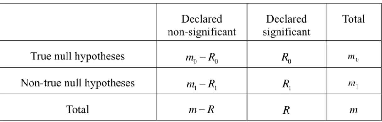
rejected hypotheses, respectively. Table 1 summarizes the four possible outcomes of the m tests.
Table 1: Possible outcomes from m hypothesis tests Declared
non-significant
Declared significant
Total
True null hypotheses m0− R0 R 0 m0
Non-true null hypotheses m1− R1 R 1 m1
The false discovery rate, FDR, is defined as the expected proportion of erroneously rejected null hypotheses. With R and R representing, respectively, the number of true null 0
hypotheses rejected and the total number of null hypotheses rejected in a multiple testing procedure, let Q =R0/R if R > 0 and Q = 0 if R = 0. Then E(Q) is the FDR. The family-wise
error rate (FWER) is defined as P( ), which is different from the “signal probability” defined as P( ). Note that when the process is in control, the FWER and the signal probability are the overall false-alarm rate.
0 1
R ≥
1
R≥
Benjamini and Hochberg (1995) also proved that:
(a) When all the null hypotheses are true, the FDR is the same as the FWER. This is obvious since in this case R0 = and thus R E Q( )=P R( ≥ =1) P R( 0 ≥ = FWER. 1)
(b) When only part of the null hypotheses are true and the others are false, the FDR is smaller than or equal to the FWER. The proof is also simple: when R0 =0, then Q= 0;
when R0 ≥1, then Q=R0/R≤ 1,Thus
0
{R 1}
I ≥ ≥ . Taking expectations on both sides leads Q
to P(R0 ≥ ≥1) E(Q).
Thus, any procedure that controls the FWER also controls the FDR. Therefore, the FDR offers a less stringent multiple-testing criterion than the FWER. The FDR may be more appropriate for some applications, particularly where a large number of null hypotheses tests are involved, for example, the microarray data analysis in bioinformatics.
Benjamini and Hochberg (1995) proved by induction that the following FDR method controls the FDR at level α when the p-values of the observed test statistics (under the null hypothesis) are independent and identically distributed as uniform [0, 1].
Step 1: Compute the p-values of the observed test statistics under the null hypothesis. Step 2: Order the p-values as p(1) ≤ ≤... p( )m .
Step 4: If k* exists, then reject the null hypotheses corresponding to {p(1),...,p( *)k };
otherwise, reject nothing.
Benjamini and Yekutieli (2001) proved that this same procedure also controls the FDR when the test statistics have positive regression dependency on each of the test statistics corresponding to the true null hypotheses. Some other related research works on FDR include Finner and Roters (2001, 2002) and Sarkar (2002).
3. The New Strategy and the OAAT Method
3.1 Traditional Method
3.1.1 Estimating Process Parameters
Assume the set of process data in Phase I is in the form of m independent random samples (each of size n) taken in the order of the process output. When the m samples are all from an in-control process, we assume ’s are independent and identically distributed as 1 { ,..., }m i in X X i=1 ij X 2 0 0 ( , ) N µ σ , for i = 1, 2, … , m and j = 1, 2, …, n.
The most commonly used estimator of µ0 is µˆ0= X = 1 1 1 1 m n 1 m ij i i j i X X mn = = m = =
∑∑
∑
, (1) where Xi is the sample mean of the ith sample. There are many estimators of σ0 given inthe literature (e.g., Champ and Chou, 2003; Nedumaran and Pignatiello, 2005). The following three variability-related statistics are considered in Champ and Chou (2003):
1 / m i i R R m = =
∑
, 1 / m i i S S = =∑
m, and 1/ 2 2 1 / m i i V S = =∑
m, (2)where R and i Si are respectively the sample range and sample standard deviation of the i
th sample with 2 1 1 ( 1 n i ij j S X n = = −
∑
−Xi) . (3)Unbiased estimators of σ0 can be obtained by rescaling these statistics as:
0 2 ˆ R d = σ , 0 4 ˆ S C = σ , and 1/ 2 0 4, ˆ m V C = σ , (4) where d2 =E R( ) /σ0 can be easily found in many quality control textbooks,
4 2 ( / 2) 1 (( 1) / 2) n C n n Γ = − Γ − , and 4, 2 (( ( 1) 1) / 2) ( 1) ( ( 1) / 2 m m n C m n m n Γ − + = − Γ − ).
Champ and Chou (2003) chose V1/ 2/C4,m as their preferred estimator of σ0 because
Var( 1/ 2 4,m V C ) ≤ Var( 4 S C ) ≤ Var( 2 R d ). (5)
Following their arguments, we let σˆ0= V1/ 2/C4,m in this paper.
3.1.2 The Control Limits of the Traditional Method
A Shewhart control chart is defined by a lower control limit (LCL), a center line (CL), and an upper control limit (UCL). These values are defined for the Phase I Shewhart X chart by 0 0 ˆ ˆ , X X LCL k n =µ − σ CLX =µˆ0, UCLX ˆ0 kX ˆ0 n =µ + σ , where 0 ˆ µ = 1 1 m i i X m
∑
= and σˆ0 =V1/ 2/C4,m.The statistic Xi (the ith sample mean) is plotted against the sample number i. If any
point falls below LCLX or above UCLX , it is taken as an evidence that the associated
sample is from an out-of-control process. For the traditional Shewhart chart, the constant kX
is usually taken as 3.
3.1.3 The Individual and the Overall False-Alarm Rate of the Traditional Method
When the m samples are all from an in-control process, Xi− is distributed as X
2 0 1 (0,m ) N m n − σ
for i = 1, 2, … , m. Note that Xi− is independent of X 2
0 ( 1) m n− V σ , which is distributed as 2 ( 1) m n−
χ , the χ2 distribution with degrees of freedom ( 1 . Therefore,
( ) ( 1) i mn X X m V − − = 2 2 0 0 ( ) / ( 1) i mn X X V m − − σ σ (6)
is distributed as tm n( −1), the distribution with degrees of freedom t m n( − )1 .
Since ( ) ( 1) X mn UCL X m V − − = 0 ˆ ( / ( 1) X mn k n m V σ − ) = 4, 1 X m k m C m− , (7)
the individual false-alarm rate is
( 1) * 4, 2(1 ( )) 1 m n X t m k m C m F α − − − = , (8) where is the cumulative distribution function of the
( −1)
m n t
F tm n( −1) distribution.
It is easy to show that the traditional method controls the overall false-alarm rate at level when the
* 1 (1− −α )m
m hypothesis tests are independent. For example, α is 0.0793 when m =30, n=5, and kX = Unfortunately, this is not the case for Phase I applications of 3.
control charts since all the tests involve some common parameter estimators. However, our simulation study indicates that the overall false-alarm rate for the case of m =30, n=5, and
3
X
k = is about 0.078, fairly close to 0.0793 for the independent tests.
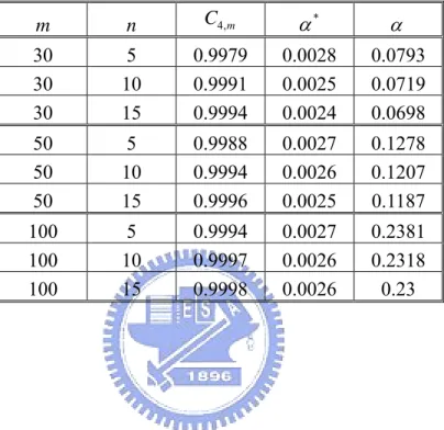
Table 2 lists the α*(individual false-alarm rate) corresponding to {
X
k =3} when the m
tests are independent. Note that the overall false-alarm rate α increases as m increases or as
n decreases.
3.2 Criteria for Performance Evaluation
As mentioned before, screening out-of-control data points is similar to finding significant hypotheses. Similar to Table 1, assume that there are in-control samples and out-of-control samples among m samples. R samples are rejected, and among them,
0
m m1
0
in-control samples are falsely rejected and R out-of-control samples are correctly rejected. 1
We shall evaluate the performance by E R( )0 and E R( )1 , the expected values of R and 0
1
R , respectively.
In Phase I, practically, we care less on the question of “whether there are any data points come from an out-of-control process” but more on “which data points come from an out-of-control process”. However, many authors evaluated the performance of a control chart by the signal probability, which can only provide a measure for the first question. Note that when the process data consist of a mixture of in-control and out-of-control data (i.e., when m > > 0), then the signal probability (denoted by P) is not the overall false-alarm rate (it is only when ) or the detecting power (only when
1
m
1 0
m = m1 = ), and alarms can be signaled m
by either true or false alarms or both. For this reason, it is somewhat questionable to evaluate the performance by the signal probability.
It seems more realistic to evaluate a control chart in Phase I analysis in terms of making more correct decisions on the state of each data point-in-control or out-of-control. Thus we propose to evaluate the performance of a monitoring scheme by the expected number of true rejections and the expected number of false rejections. The former has the same flavor as the Type I error in the hypothesis testing and the latter is more or less measuring the detecting power of the scheme.
3.2.1 A Simulation Study
Many SPC books have recommended that 20-30 subgroups of size 4 or 5 be used for estimating the process parameters (see, e.g., Montgomery, 2005). Thus, we choose the setting of m =30, n=5, and kX = for illustrating the behaviors of the above criteria in our 3 simulation study. Without loss of generality, we can let µ0=0 and σ0=1.
Consider m1 = 0, 3, 6, 9, 12 and δ = 0 (0.4) 4 (that is, m1 subgroups shift from µ0
dataset produces its own R and 0 R . When 1 R0+R1 > the alarm signals. We estimate the 0,
signal probability P by , the sample proportion of such signals among the 1,000,000 datasets. Let
ˆP 0
R , the average of the 1,000,000 R ’s, be the estimate of 0 E R( )0 , and R1, the
average of the 1,000,000 R ’s, be the estimate of 1 E R( )1 .
For the 41 combinations of m1 and δ considered, the standard errors of the are about 0-0.00049, and the standard errors of the
ˆP 0
R and R1 are about 0-0.00227. Table 3
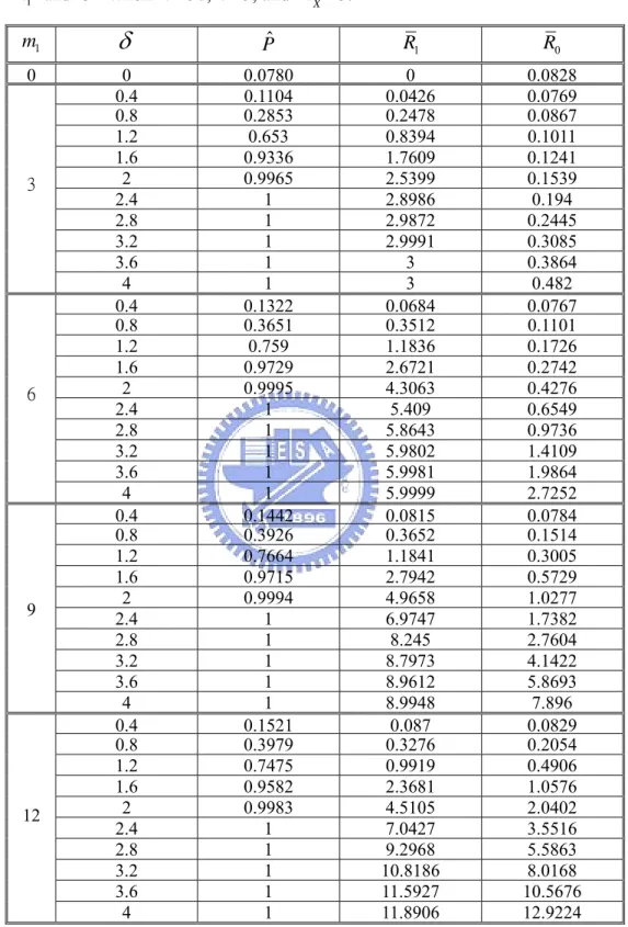
shows the values of , ˆP R0, and R1. The following observations can be made from the
results displayed.
(a) For (i.e. the process is in control), , the estimate of the overall false-alarm rate, is about 0.078, which is quite close to the nominal value 0.079.
1 0
m = ˆP
(b) For m1=0, R0 is 0.0828, which is greater than =0.078. The reason is that when
an alarm signals,
ˆP 0
R ≥ 1, while in estimating traditional overall false-alarm rate P, the
signaling alarm only counts one no matter how many points are beyond the control limits. (c) As expected, R1 increases as the size of the shift δ increases, but R0 increases as
well-this is the cost of instability.
(d) R1 moves in the same direction as , and yet it contains more information than .
It indicates, in the average, how many true out-of-control samples the method can detect. On the other hand,
ˆP ˆP
0
R can measure how often false alarms can occur. As to , recall that when
, is just the alarm signaling rate, and the alarm for each dataset can be triggered by samples from either state.
ˆP 1
0 m< <m ˆP
3.3 The Performance of the OAAT/Traditional Procedure
As mentioned before, there may be some out-of-control samples undetected at each iteration of the control chart construction, especially when the preliminary control limits are constructed using a set of data contaminated by some out-of-control samples. These out-of-control samples often inflate the estimate of σ0, which makes the control limits too wide. If we inspect the process looking for assignable causes for each of the alarms whenever it signals, as the current practice suggests, the number of times of stop-and-inspect may be unnecessarily high. Here we suggest a new strategy: run through the whole iterative procedure by removing all beyond-limits points at each iteration, and then perform the inspection for assignable causes at the end.
By examining the results of the above practice, it is found that the number of false alarms is higher than we would expect. To reduce the wasteful false alarms, we propose and study a new practice-discard only one sample at a time instead of discarding all in the traditional method. Our simulation study shows that this OAAT/traditional procedure can reduce the number of false alarms dramatically, which in turn will reduce the amount of time in conducting unnecessary investigations for non-existing assignable causes and reserve more in-control data for more efficient process modeling. The main reason why this procedure works is that the most extreme point is more likely to be an out-of-control sample compared to others. In contrast, the traditional method discards all the samples beyond the control limits at each iteration, thus there is more chance that some may be in-control samples.
3.3.2 The OAAT Procedure
We describe the OAAT/traditional procedure below:
Step 1. Construct the preliminary control limits with all collected data.
Step 2. If no out-of-control samples are identified, stop iterating and go to Step 4; otherwise, discard the most extreme sample.
Step 3. Construct the preliminary control limits with the remaining samples; go to Step 2.
Step 4. Collect all the samples discarded in the above iterations and inspect the process for assignable causes.
3.3.3 The Simulation Study
Set m=30, 50, 100 and n=5, 10, 15. For each combination, consider the situations = 0.1m, 0.2m, 0.3m, 0.4m and
1
m
δ = 0.4 (0.4) 4. For each case considered, simulate 1,000,000 datasets and calculate R0 and R1 as described before. The estimated standard errors of R0
and R1 are about 0-0.0069.
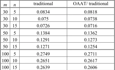
Table 4 gives the R0 of the two procedures (traditional vs. OAAT/traditional) when all
the m samples are from the in-control process. Note that the R0 of the OAAT/traditional
procedure is less than the traditional method in every case considered. This means that the OAAT/traditional procedure will signals fewer false alarms.
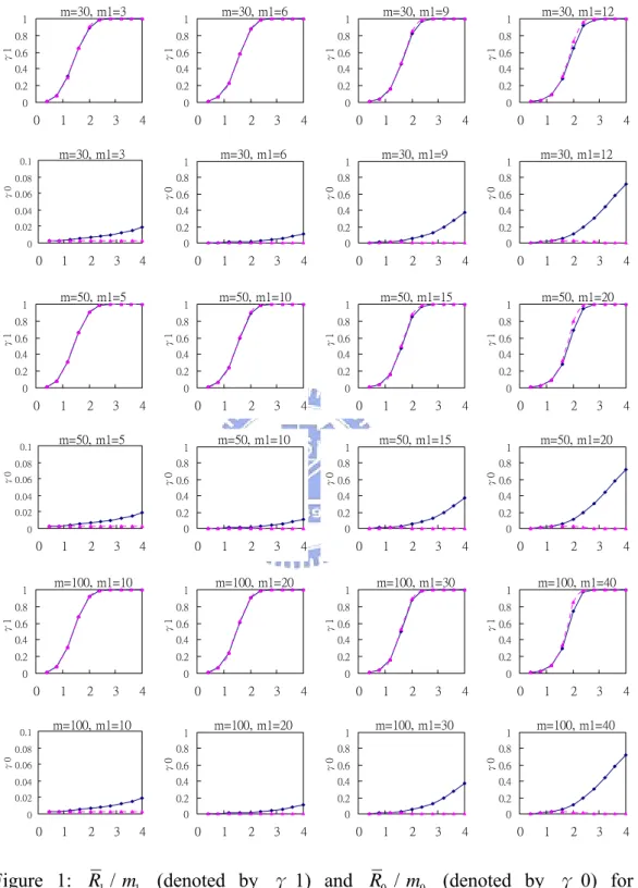
For n = 5, 10, 15, Figures 1-3 respectively plot the simulated R1/m1and R0/m0 versus
δ for various values of m and . The following observations can be made from the results displayed.
1
m
(a) The performance of the OAAT/traditional procedure in terms of R1/ is slightly
better than that of the traditional method in general. And, for fixed m, the advantage increases as increases.
1
m
1
m
(b) The R0/ of the OAAT/traditional procedure is uniformly smaller than that of the
traditional method. And, for fixed m, the advantage increases as increases. Note that all the 0 m 1 m 0
R / curves of the OAAT/traditional procedure lie almost flat on x-axis, which means
the new procedure seldom signals false alarms. 0
m
(c) From figures we can see that the improvement of the OAAT procedure in some situations is extremely large.
In summary, the OAAT/traditional method offers a good alternative to the traditional method for practical use. It is as powerful as the traditional method, but can diminish the false-alarm rate dramatically.
The number of samples m also plays an important role on the extent of the improvement of the OAAT procedure. We study the effect of m in the next subsection.
3.4 The Effect of m
Since the overall false-alarm rate increases when the number of samples m increases, we use the Bonferroni method to control the family-wise error rate α in this Subsection.
3.4.1 The Simulation Study
Let kX = (m−1) /mC4,m m nt ( −1), / 2α m. The value tν,1−γ is the 100γth percentile of a t
distribution with ν degrees of freedom. Letα =0.05. We list the value of kX in Table 5.
Note that kX increases as m increases or as n decreases.
In this study, we simulate 1,000,000 datasets using the same setting as given in Subsection 3.3.3 and calculate R0 and R1 for each situation considered. The standard errors
of R0 and R1 are about 0-0.00998.
Table 6 gives R0 when all the m samples are from the in-control process. The R0 of
the OAAT/Bonferroni procedure is smaller than that of the Bonferroni method in each situation.
For n = 5, 10, 15, Figures 4-6 respectively plot the simulated R1/m1and R0/ values
versus
0
m
δ for various values of m and . The following observations can be made from the results displayed.
1
m
effect of multiplicity control, which means that for controlling a fixed overall false-alarm rate (α ) for m samples, the individual false-alarm rate ( ) gets smaller as m increases,hence the number of beyond-limits points also gets smaller as m increases.
* / m
α =α
(b) The R0/ of each of the both procedures decreases when m increases-the reason
is similar to (a). 0
m
(c) The performance of the OAAT/Bonferroni procedure in terms of R1/ is about the
same as the Bonferroni method.
1
m
(d) The OAAT/Bonferroni procedure performs much better in terms of R0/ than the
Bonferroni method. However, the advantage decreases as m increases. This is because when
m increases, fewer false alarms can occur for the Bonferroni method but the OAAT procedure
already has very few false alarms, thus the difference between the two methods becomes smaller. In other words, the effect of multiplicity control is more for the Bonferroni method than for the OAAT/ Bonferroni procedure.
0
m
In summary, applying the OAAT procedure to the Bonferroni method has the advantage of reducing the number of false alarms dramatically, while retaining a similar power of detecting out-of-control samples.
4. The FDR Method and the OAAT/FDR Procedure
4.1 Bonferroni Method
To control the overall false alarm at a desired level α, the most common practice for testing m hypotheses simultaneously is the Bonferroni method, which simply controls the individual false-alarm rate at level α* =α/ m.
Recall that mn X( i−X) / (m−1) V is distributed as tm n( −1), the distribution with
degrees of freedom . It is easy to show that the control limits for the Bonferroni method are t ( 1 m n− ) * ( 1), / 2 1 m n m V X t mn α − − ± , (9)
where α* is the individual false-alarm rate.
4.2 Comparing Bonferroni and FDR Methods
This subsection compares the performance of the Bonferroni method and the FDR method in terms of the signal probability P, E R( )0 , and E R( )1 .
4.2.1 The Simulation Study
In this study, we set α =0.05 and α*= . Consider m = 30, n = 5, = 0, 3, 6, 9, 12, and
0.05 / m m1
δ = 0 (0.4) 4. Simulate 1,000,000 datasets and calculate , ˆP R0, and R1 for each
combination considered. The standard errors of the are about 0-0.000496, and the standard errors of
ˆP 0
R and R1 are about 0-0.00267.
Table 7 and Figure 7 show the simulated , ˆP R0 and R1 for m1 = 0, 3, 6, 9, 12 and
δ = 0 (0.4) 4. The following observations can be made from the results displayed.
the Bonferroni method is smaller than that of the FDR method. Although they both control the overall false-alarm rate at level 0.05, the former is more conservative.
(b) R1 of the FDR method is uniformly larger than that of the Bonferroni method and
the advantage increases as m1 or δ increases. So, the former is more powerful.
(c) But R0 of the FDR method is also uniformly larger than that of the Bonferroni
method. And, the disadvantage increases as m1 or δ increases.
Benjamini and Hochberg (1995) indicated that the FDR method is much more powerful than comparable procedures controlling the traditional family-wise error (the overall false-alarm rate when all the samples are in control). However, here we find in (c) that the performance of the FDR method in terms of is worse than that of the Bonferroni method. This is similar to the relationship between the Type I and Type II errors in testing hypothesis.
0 ( )
E R
The number of samples m is also an important factor, especially in genetic research. Benjamini and Hochberg (1995) showed by simulation that the power of the FDR method in terms of the signal probability is uniformly larger than the Bonferroni method and the advantage increases in m as well as m1/m.
We investigate the effect of the OAAT procedure when applied on the FDR method in the next section.
4.3 The Performance of the OAAT/FDR Procedure
Here, we apply the OAAT procedure to the FDR method by discarding only the sample with the minimum p-value in each iteration.
4.3.1 The Simulation Study
In this study, we simulate 1,000,000 datasets using the same setting as given in Subsection 3.3.3 and calculate R0 and R1 for each situation considered. The standard errors
of R0 and R1 are about 0-0.0093.
Table 8 gives the R0 of the three procedures (Bonferroni, FDR, and OAAT/FDR) when
all the m samples are from the in-control process. Note that the R0 of the OAAT/FDR
procedure is uniformly smaller than that of the FDR method, but larger than that of the Bonferroni method in each situation. This means that the OAAT/FDR procedure signals fewer false alarms than the FDR method, but signals more than the Bonferroni method, which is because the Bonferroni method is very conservative.
For n = 5, 10, 15, Figures 8-10 respectively plot the simulated R1/m1and R0/m0 versus
δ for various values of m and . The following observations can be made from the results displayed.
1
m
(a) The R1/ of each of the three procedures decreases in general as m increases, but
increase as n increases. 1
m
(b) The R0/m0 of each of the three procedures decreases as m increases.
(c) The R0/ of the Bonferroni method increases as n increases and the same for the
FDR method, but the 0
m
0
R /m0 of the OAAT/FDR procedure decreases in most cases.
(d) The OAAT/FDR procedure performs about the same as the FDR method in terms of 1
R/ . The advantage increases as increases and increases in most cases as m increases
or n decreases. 1
m m1
(e) The R0/ of the OAAT/FDR procedure is uniformly smaller than that of the FDR
method. Also, the advantage increases as or n increases, but decreases in most cases as m increases. Note that the performance of the OAAT/FDR procedure is much better than that of the FDR method.
0
m
1
(f) Except for a small number of cases, the R1/ of the OAAT/FDR procedure is
larger than that of the Bonferroni method. The advantage increases as increases and increases in most cases as m increases or n decreases.
1
m
1
m
(g) The R0/ of the OAAT/FDR procedure is much smaller than the Bonferroni
method in most cases. And, the advantage increases as or n increases, but decreases as m increases.
0
m
1
m
In summary, applying the OAAT procedure to any control schemes has the advantage of reducing the number of false alarms dramatically, while retaining the similar power of detecting out-of-control samples.
5. Conclusions
In this paper, we study some strategies of Phase I analysis in control charting. It is found that the practice of discarding all beyond-limits samples at each iteration in constructing appropriate control charts has a major drawback of throwing away too many in-control samples. To overcome this drawback, we propose and study in this paper a new OAAT procedure that only discards the most extreme sample at a time. Our simulation study demonstrates that the OAAT procedure reduces dramatically the occurrences of such false alarms. And this advantage is more profound when the process is more unstable (i.e., more out-of-control samples or largerδ ).
We also suggest a new strategy on when to inspect the process to look for assignable causes for samples signaling out-of-control alarms-instead of performing stop-and-inspect whenever alarms signal. The new strategy is: run through the whole iterative procedure by removing beyond-limits points one at a time at each iteration and then perform the investigation for all alarms after all the remaining samples are all in control. This practice may save tremendous amount of time and money in bringing process to in-control state.
We study three approaches of error control-the traditional method, Bonferroni method, and FDR method. They control, respectively, the individual false-alarm rate, the overall false-alarm rate, and the false discovery rate. The individual false-alarm rate of the traditional method is kept fixed for each sample at each iteration, but this rate of the other two methods becomes larger when more beyond-limits samples are removed as the screening process progresses.
Under the same overall false-alarm rate, the FDR method is more powerful than the Bonferroni method, but mistaken more in-control samples for being out of control. The OAAT procedure can overcome this problem.
considered in the literature, including signal probability (P( )), FWER (P( )), FDR (E
1
R≥ R0 ≥1
0
(R / )R ), and the E(R ) and E(0 R ) (or E(1 R0/m ) and E(0 R m )) suggested in this paper. 1/ 1
The signal probability considers “the process” as a whole. It only assesses the ability of judging if a process is in control or not. It does not assess the scheme on its performance of screening out out-of-control samples and/or keeping in-control points. The FWER and FDR emphasize more on the false-alarm rate of the scheme. With a mixture of in-control and out-of-control samples in the dataset, perhaps it is more appropriate to use two indicators- one to assess the false-alarm rate and the other to assess the detection power, such as E(R ) 0
and E(R ) (or E(1 R0/m ) and E(0 R m )). E(1/ 1 R ) and E(0 R ) assess false alarms and true alarms 1
separately, and they can distinguish between cases with different numbers of alarms.
The X chart used in this paper is just for demonstration of the above ideas. The new strategy of Phase I analysis, evaluation criteria for control schemes, and the new OAAT procedure can be applied to any other control charts.
References
[1] Albers, W. and Kallenberg, W. C. M. (2004a). “Estimation in Shewhart Control Charts”.
Metrika 59: 207-234.
[2] Albers, W. and Kallenberg, W. C. M. (2004b). “Are Estimated Control Charts in Control”.
Statistics 38: 67-79.
[3] Benjamini, Y. and Hochberg, Y. (1995). “Controlling the False Discovery Rate: A Practical and Powerful Approach to Multiple Testing”. Journal of Royal Statistical
Society, B. 57:289-300.
[4] Benjamini, Y. and Yekutieli, D. (2001). “The Control of the False Discovery Rate in the Multiple Testing Under Dependency”. Annals of Statistics 29:1165-1188.
[5] Borror, C. M. and Champ, C. W. (2001). “Phase I Control Charts for Independent Bernoulli Data”. Quality and Reliability Engineering International 17: 391–396.
[6] Champ, C. W. and Chou, S.-P. (2003). “Comparison of Standard and Individual Limits Phase I Shewhart X , R, and S Charts”. Quality and Reliability Engineering
International 19:161–170.
[7] Champ, C. W. and Jones, L. A. (2004). “Designing Phase I X Charts with Small Sample Sizes”. Quality and Reliability Engineering International 20:497–510.
[8] Finner, H. and Roters, M. (2001). “On the False Discovery Rate and Expected Type I Errors”. Biometrical Journal 43:985-1005.
Type I Errors”. Ann. Statist. 30:220-238.
[10] Hoyer, R. W. and Ellis, W. C. (1996a). “A Graphical Exploration of SPC, Part 1”.
Quality Progress 65–73.
[11] Hoyer, R. W. and Ellis, W. C. (1996b). “A Graphical Exploration of SPC, Part 2”.
Quality Progress 57–64.
[12] Hoyer, R. W. and Ellis, W. C. (1996c). “Another Look at a Graphical Exploration of SPC”. Quality Progress 85–93.
[13] Hunter, J. S. (1998). “The Box-Jenkins Manual Adjustment Chart”. Quality Progress 129–137.
[14] Jones, L. A. and Champ, C. W. (2002). “Phase I Control Charts for Times between Events”. Quality and Reliability Engineering International 18:479 - 488.
[15] Juran, J. M. (1997). “Early SQC: A Historical Supplement”. Quality Progress 73–81.
[16] Mahmoud, M. A. and Woodall, W. H. (2004). “Phase I Analysis of Linear Profiles with Calibration Applications”. Technometrics 46:380-391.
[17] Montgomery D. C. (2005). Introduction to Statistical Quality Control, 5th
Edition. Wiley:
New York.
[18] Nedumaran, G. and Pignatiello, J. J. (2000). “On Constructing T2 Control Charts for Retrospective Examination”. Communications in Statistics–Simulation and
[19] Nedumaran, G. and Pignatiello, J. J. (2001). “On Estimating X Control Chart Limits”.
Journal of Quality Technology 33:206-212.
[20] Nedumaran, G. and Pignatiello, J. J. (2005). “On Constructing Retrospective X Control Chart Limits”. Quality and Reliability Engineering International 21:81–89.
[21] Nelson, L. S. (1999). “Notes on the Shewhart Control Chart”. Journal of Quality
Technology 31:124–126.
[22] Reynolds, M. R. Jr. and Stoumbos Z. G. (2001). “Monitoring the Process Mean and Variance Using Individual Observations and Variable Sampling Intervals”. Journal of
Quality Technology 33:181–205.
[23] Sarkar, S. K. (2002). “Some Results on False Discovery Rate in Stepwise Multiple Testing Procedures”. The Annals of Statistics 30(1):239–257.
[24] Sullivan, J. H. and Woodall, W. H. (1996). “A Control Chart for Preliminary Analysis of Individual Observations”. Journal of Quality Technology 28:265-278.
[25] Vermaat, M. B., Ion, R. A., Does, R. J. M. M. and Klaassen, C. A. J. (2003). “A Comparison of Shewhart Individuals Control Charts Based on Normal, Nonparametric, and Extreme-Value Theory”. Quality and Reliability Engineering International 19:337–353
[26] Woodall, W. H. and Montgomery, D. C. (1999). “Research Issues and Ideas in Statistical Process Control”. Journal of Quality Technology 31(4):377–386.
Tables
Table 2: The individual false alarm rate (α*) and the overall false-alarm rate (α ) for various m and n when kX =3.
m n C4,m α* α 30 5 0.9979 0.0028 0.0793 30 10 0.9991 0.0025 0.0719 30 15 0.9994 0.0024 0.0698 50 5 0.9988 0.0027 0.1278 50 10 0.9994 0.0026 0.1207 50 15 0.9996 0.0025 0.1187 100 5 0.9994 0.0027 0.2381 100 10 0.9997 0.0026 0.2318 100 15 0.9998 0.0026 0.23
Table 3: ˆP, R1, and R0 of the traditional method based on 1,000,000 replications for
various m1 and
δ
when m =30, n =5, and kX =3.1 m
δ
ˆP R1 R0 0 0 0.0780 0 0.0828 0.4 0.1104 0.0426 0.0769 0.8 0.2853 0.2478 0.0867 1.2 0.653 0.8394 0.1011 1.6 0.9336 1.7609 0.1241 2 0.9965 2.5399 0.1539 2.4 1 2.8986 0.194 2.8 1 2.9872 0.2445 3.2 1 2.9991 0.3085 3.6 1 3 0.3864 3 4 1 3 0.482 0.4 0.1322 0.0684 0.0767 0.8 0.3651 0.3512 0.1101 1.2 0.759 1.1836 0.1726 1.6 0.9729 2.6721 0.2742 2 0.9995 4.3063 0.4276 2.4 1 5.409 0.6549 2.8 1 5.8643 0.9736 3.2 1 5.9802 1.4109 3.6 1 5.9981 1.9864 6 4 1 5.9999 2.7252 0.4 0.1442 0.0815 0.0784 0.8 0.3926 0.3652 0.1514 1.2 0.7664 1.1841 0.3005 1.6 0.9715 2.7942 0.5729 2 0.9994 4.9658 1.0277 2.4 1 6.9747 1.7382 2.8 1 8.245 2.7604 3.2 1 8.7973 4.1422 3.6 1 8.9612 5.8693 9 4 1 8.9948 7.896 0.4 0.1521 0.087 0.0829 0.8 0.3979 0.3276 0.2054 1.2 0.7475 0.9919 0.4906 1.6 0.9582 2.3681 1.0576 2 0.9983 4.5105 2.0402 2.4 1 7.0427 3.5516 2.8 1 9.2968 5.5863 3.2 1 10.8186 8.0168 3.6 1 11.5927 10.5676 12 4 1 11.8906 12.9224Table 4: R0of the traditional method and the OAAT/traditional procedure when all the
samples are in control for various combinations of m and n.
m n traditional OAAT/ traditional
30 5 0.0834 0.0818 30 10 0.075 0.0738 30 15 0.0726 0.0716 50 5 0.1384 0.1362 50 10 0.1291 0.1273 50 15 0.1271 0.1254 100 5 0.2749 0.2711 100 10 0.2651 0.2617 100 15 0.2639 0.2606
Table 5: kX for various m and n when the overall false-alarm rate α is at 0.05.
m n α α*(α /m) k X 30 5 0.05 0.0017 3.1561 30 10 0.05 0.0017 3.1197 30 15 0.05 0.0017 3.1094 50 5 0.05 0.001 3.3021 50 10 0.05 0.001 3.2772 50 15 0.05 0.001 3.2701 100 5 0.05 0.0005 3.4897 100 10 0.05 0.0005 3.4750 100 15 0.05 0.0005 3.4708
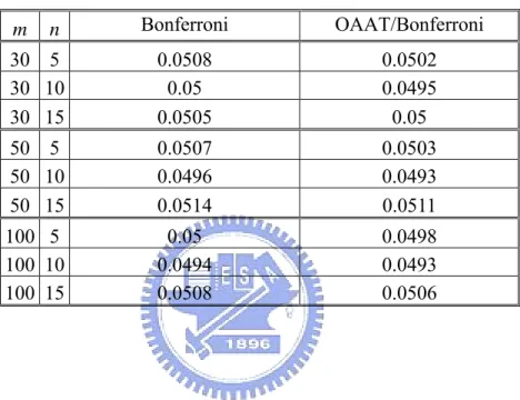
Table 6: R0 of the Bonferroni method and the OAAT/Bonferroni procedure when all
the samples are in-control for various combinations of m and n.
m n Bonferroni OAAT/Bonferroni 30 5 0.0508 0.0502 30 10 0.05 0.0495 30 15 0.0505 0.05 50 5 0.0507 0.0503 50 10 0.0496 0.0493 50 15 0.0514 0.0511 100 5 0.05 0.0498 100 10 0.0494 0.0493 100 15 0.0508 0.0506
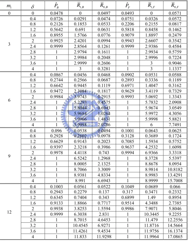
Table 7: ˆP, R1 and R0 between the Bonferroni method and the FDR method when m =30 and n =5. 1 m δ PˆB R1,B R0,B PˆF R1,F R0,F 0 0 0.0478 0 0.0497 0.0493 0 0.0571 0.4 0.0726 0.0291 0.0474 0.0751 0.0326 0.0572 0.8 0.2126 0.1853 0.0533 0.2206 0.2155 0.0817 1.2 0.5642 0.691 0.0631 0.5818 0.8458 0.1462 1.6 0.8955 1.5766 0.0776 0.9079 1.8897 0.2479 2 0.9925 2.4201 0.0994 0.9943 2.6607 0.3542 2.4 0.9999 2.8564 0.1261 0.9999 2.9386 0.4584 2.8 1 2.9794 0.1611 1 2.9934 0.5759 3.2 1 2.9984 0.2048 1 2.9996 0.7224 3.6 1 2.9999 0.2606 1 3 0.9046 3 4 1 3 0.3281 1 3 1.1337 0.4 0.0867 0.0456 0.0468 0.0902 0.0531 0.0588 0.8 0.2744 0.2566 0.0687 0.2893 0.3336 0.1189 1.2 0.6642 0.9445 0.1119 0.6971 1.4047 0.3162 1.6 0.9472 2.3084 0.1817 0.9629 3.4119 0.7329 2 0.9984 3.9743 0.2915 0.9993 5.0692 1.3343 2.4 1 5.2293 0.4575 1 5.7832 2.0908 2.8 1 5.8044 0.6943 1 5.9674 3.0549 3.2 1 5.9684 1.0264 1 5.9972 4.3056 3.6 1 5.9966 1.4831 1 5.9998 5.8821 6 4 1 5.9998 2.0786 1 6 7.7491 0.4 0.096 0.0538 0.0494 0.1001 0.0643 0.0625 0.8 0.2928 0.2602 0.0978 0.3128 0.3689 0.1724 1.2 0.6629 0.9143 0.2023 0.7085 1.5934 0.5752 1.6 0.9397 2.3218 0.3986 0.9637 4.2532 1.6098 2 0.9978 4.4118 0.743 0.9994 6.9366 3.3318 2.4 1 6.5242 1.2968 1 8.3728 5.5397 2.8 1 8.0005 2.1325 1 8.8678 8.0954 3.2 1 8.7066 3.3009 1 8.9814 10.8182 3.6 1 8.9381 4.8334 1 8.9983 13.4291 9 4 1 8.991 6.6943 1 8.9999 15.7008 0.4 0.1003 0.0561 0.0522 0.1049 0.0689 0.066 0.8 0.2943 0.2279 0.137 0.317 0.3471 0.2332 1.2 0.6345 0.7404 0.343 0.6899 1.49 0.8954 1.6 0.9133 1.8866 0.7717 0.9514 4.3488 2.7385 2 0.9938 3.8253 1.5594 0.9986 7.9071 5.8046 2.4 0.9999 6.3038 2.831 1 10.3445 9.2255 2.8 1 8.7015 4.6453 1 11.479 12.2556 3.2 1 10.4545 6.9271 1 11.8716 14.5664 3.6 1 11.4261 9.4534 1 11.9756 16.1374 12 4 1 11.833 11.9298 1 11.9964 17.0865
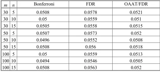
Table 8: R0 of the Bonferroni method, the FDR method, and the OAAT/FDR procedure
when all the samples are from the in-control process for various combinations of m and n.
m n Bonferroni FDR OAAT/FDR 30 5 0.0508 0.0578 0.0521 30 10 0.05 0.0559 0.051 30 15 0.0505 0.0558 0.0515 50 5 0.0507 0.0573 0.052 50 10 0.0496 0.0552 0.0508 50 15 0.0508 0.056 0.0518 100 5 0.05 0.0559 0.0513 100 10 0.0494 0.0546 0.0505 100 15 0.0508 0.0563 0.052
Figures
m=30, m1=3 0 0.2 0.4 0.6 0.8 1 0 1 2 3 4 γ1 m=30, m1=6 0 0.2 0.4 0.6 0.8 1 0 1 2 3 4 γ1 m=30, m1=9 0 0.2 0.4 0.6 0.8 1 0 1 2 3 4 γ1 m=30, m1=12 0 0.2 0.4 0.6 0.8 1 0 1 2 3 4 γ1 m=30, m1=3 0 0.02 0.04 0.06 0.08 0.1 0 1 2 3 4 γ0 m=30, m1=6 0 0.2 0.4 0.6 0.8 1 0 1 2 3 4 γ0 m=30, m1=9 0 0.2 0.4 0.6 0.8 1 0 1 2 3 4 γ0 m=30, m1=12 0 0.2 0.4 0.6 0.8 1 0 1 2 3 4 γ0 m=50, m1=5 0 0.2 0.4 0.6 0.8 1 0 1 2 3 4 γ1 m=50, m1=10 0 0.2 0.4 0.6 0.8 1 0 1 2 3 4 γ1 m=50, m1=15 0 0.2 0.4 0.6 0.8 1 0 1 2 3 4 γ1 m=50, m1=20 0 0.2 0.4 0.6 0.8 1 0 1 2 3 4 γ1 m=50, m1=5 0 0.02 0.04 0.06 0.08 0.1 0 1 2 3 4 γ0 m=50, m1=10 0 0.2 0.4 0.6 0.8 1 0 1 2 3 4 γ0 m=50, m1=15 0 0.2 0.4 0.6 0.8 1 0 1 2 3 4 γ0 m=50, m1=20 0 0.2 0.4 0.6 0.8 1 0 1 2 3 4 γ0 m=100, m1=10 0 0.2 0.4 0.6 0.8 1 0 1 2 3 4 γ1 m=100, m1=20 0 0.2 0.4 0.6 0.8 1 0 1 2 3 4 γ1 m=100, m1=30 0 0.2 0.4 0.6 0.8 1 0 1 2 3 4 γ1 m=100, m1=40 0 0.2 0.4 0.6 0.8 1 0 1 2 3 4 γ1 m=100, m1=10 0 0.02 0.04 0.06 0.08 0.1 0 1 2 3 4 γ0 m=100, m1=20 0 0.2 0.4 0.6 0.8 1 0 1 2 3 4 γ0 m=100, m1=30 0 0.2 0.4 0.6 0.8 1 0 1 2 3 4 γ0 m=100, m1=40 0 0.2 0.4 0.6 0.8 1 0 1 2 3 4 γ0Figure 1: R1/ m1 (denoted by γ1) and R0 / (denoted by γ0) for various combinations of m and (n=5). The x-axis is the shift size
0
m
1
m δ . The solid line with
diamonds corresponds to the traditional method and the dashed line with triangles corresponds to the OAAT/traditional procedure.
m=30, m1=3 0 0.2 0.4 0.6 0.8 1 0 1 2 3 4 γ1 m=30, m1=6 0 0.2 0.4 0.6 0.8 1 0 1 2 3 4 γ1 m=30, m1=9 0 0.2 0.4 0.6 0.8 1 0 1 2 3 4 γ1 m=30, m1=12 0 0.2 0.4 0.6 0.8 1 0 1 2 3 4 γ1 m=30, m1=3 0 0.02 0.04 0.06 0.08 0.1 0 1 2 3 4 γ0 m=30, m1=6 0 0.2 0.4 0.6 0.8 1 0 1 2 3 4 γ0 m=30, m1=9 0 0.2 0.4 0.6 0.8 1 0 1 2 3 4 γ0 m=30, m1=12 0 0.2 0.4 0.6 0.8 1 0 1 2 3 4 γ0 m=50, m1=5 0 0.2 0.4 0.6 0.8 1 0 1 2 3 4 γ1 m=50, m1=10 0 0.2 0.4 0.6 0.8 1 0 1 2 3 4 γ1 m=50, m1=15 0 0.2 0.4 0.6 0.8 1 0 1 2 3 4 γ1 m=50, m1=20 0 0.2 0.4 0.6 0.8 1 0 1 2 3 4 γ1 m=50, m1=5 0 0.02 0.04 0.06 0.08 0.1 0 1 2 3 4 γ0 m=50, m1=10 0 0.2 0.4 0.6 0.8 1 0 1 2 3 4 γ0 m=50, m1=15 0 0.2 0.4 0.6 0.8 1 0 1 2 3 4 γ0 m=50, m1=20 0 0.2 0.4 0.6 0.8 1 0 1 2 3 4 γ0 m=100, m1=10 0 0.2 0.4 0.6 0.8 1 0 1 2 3 4 γ1 m=100, m1=20 0 0.2 0.4 0.6 0.8 1 0 1 2 3 4 γ1 m=100, m1=30 0 0.2 0.4 0.6 0.8 1 0 1 2 3 4 γ1 m=100, m1=40 0 0.2 0.4 0.6 0.8 1 0 1 2 3 4 γ1 m=100, m1=10 0 0.02 0.04 0.06 0.08 0.1 0 1 2 3 4 γ0 m=100, m1=20 0 0.2 0.4 0.6 0.8 1 0 1 2 3 4 γ0 m=100, m1=30 0 0.2 0.4 0.6 0.8 1 0 1 2 3 4 γ0 m=100, m1=40 0 0.2 0.4 0.6 0.8 1 0 1 2 3 4 γ0
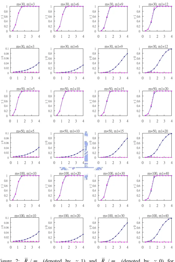
Figure 2: R1/ m1 (denoted by γ1) and R0 / (denoted by γ0) for various combinations of m and (n=10). The x-axis is the shift size
0
m
1
m δ . The solid line with
diamonds corresponds to the traditional method and the dashed line with triangles corresponds to the OAAT/traditional procedure.
m=30, m1=3 0 0.2 0.4 0.6 0.8 1 0 1 2 3 4 γ1 m=30, m1=6 0 0.2 0.4 0.6 0.8 1 0 1 2 3 4 γ1 m=30, m1=9 0 0.2 0.4 0.6 0.8 1 0 1 2 3 4 γ1 m=30, m1=12 0 0.2 0.4 0.6 0.8 1 0 1 2 3 4 γ1 m=30, m1=3 0 0.02 0.04 0.06 0.08 0.1 0 1 2 3 4 γ0 m=30, m1=6 0 0.2 0.4 0.6 0.8 1 0 1 2 3 4 γ0 m=30, m1=9 0 0.2 0.4 0.6 0.8 1 0 1 2 3 4 γ0 m=30, m1=12 0 0.2 0.4 0.6 0.8 1 0 1 2 3 4 γ0 m=50, m1=5 0 0.2 0.4 0.6 0.8 1 0 1 2 3 4 γ1 m=50, m1=10 0 0.2 0.4 0.6 0.8 1 0 1 2 3 4 γ1 m=50, m1=15 0 0.2 0.4 0.6 0.8 1 0 1 2 3 4 γ1 m=50, m1=20 0 0.2 0.4 0.6 0.8 1 0 1 2 3 4 γ1 m=50, m1=5 0 0.02 0.04 0.06 0.08 0.1 0 1 2 3 4 γ0 m=50, m1=10 0 0.2 0.4 0.6 0.8 1 0 1 2 3 4 γ0 m=50, m1=15 0 0.2 0.4 0.6 0.8 1 0 1 2 3 4 γ0 m=50, m1=20 0 0.2 0.4 0.6 0.8 1 0 1 2 3 4 γ0 m=100, m1=10 0 0.2 0.4 0.6 0.8 1 0 1 2 3 4 γ1 m=100, m1=20 0 0.2 0.4 0.6 0.8 1 0 1 2 3 4 γ1 m=100, m1=30 0 0.2 0.4 0.6 0.8 1 0 1 2 3 4 γ1 m=100, m1=40 0 0.2 0.4 0.6 0.8 1 0 1 2 3 4 γ1 m=100, m1=10 0 0.02 0.04 0.06 0.08 0.1 0 1 2 3 4 γ0 m=100, m1=20 0 0.2 0.4 0.6 0.8 1 0 1 2 3 4 γ0 m=100, m1=30 0 0.2 0.4 0.6 0.8 1 0 1 2 3 4 γ0 m=100, m1=40 0 0.2 0.4 0.6 0.8 1 0 1 2 3 4 γ0
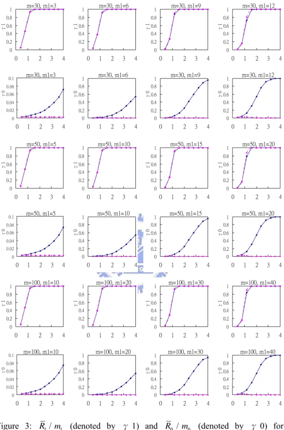
Figure 3: R1/ m1 (denoted by γ1) and R0 / (denoted by γ0) for various combinations of m and (n=15). The x-axis is the shift size
0
m
1
m δ . The solid line with
diamonds corresponds to the traditional method and the dashed line with triangles corresponds to the OAAT/traditional procedure.
m=30, m1=3 0 0.2 0.4 0.6 0.8 1 0 1 2 3 4 γ1 m=30, m1=6 0 0.2 0.4 0.6 0.8 1 0 1 2 3 4 γ1 m=30, m1=9 0 0.2 0.4 0.6 0.8 1 0 1 2 3 4 γ1 m=30, m1=12 0 0.2 0.4 0.6 0.8 1 0 1 2 3 4 γ1 m=30, m1=3 0 0.02 0.04 0.06 0.08 0.1 0 1 2 3 4 γ0 m=30, m1=6 0 0.2 0.4 0.6 0.8 1 0 1 2 3 4 γ0 m=30, m1=9 0 0.2 0.4 0.6 0.8 1 0 1 2 3 4 γ0 m=30, m1=12 0 0.2 0.4 0.6 0.8 1 0 1 2 3 4 γ0 m=50, m1=5 0 0.2 0.4 0.6 0.8 1 0 1 2 3 4 γ1 m=50, m1=10 0 0.2 0.4 0.6 0.8 1 0 1 2 3 4 γ1 m=50, m1=15 0 0.2 0.4 0.6 0.8 1 0 1 2 3 4 γ1 m=50, m1=20 0 0.2 0.4 0.6 0.8 1 0 1 2 3 4 γ1 m=50, m1=5 0 0.02 0.04 0.06 0.08 0.1 0 1 2 3 4 γ0 m=50, m1=10 0 0.2 0.4 0.6 0.8 1 0 1 2 3 4 γ0 m=50, m1=15 0 0.2 0.4 0.6 0.8 1 0 1 2 3 4 γ0 m=50, m1=20 0 0.2 0.4 0.6 0.8 1 0 1 2 3 4 γ0 m=100, m1=10 0 0.2 0.4 0.6 0.8 1 0 1 2 3 4 γ1 m=100, m1=20 0 0.2 0.4 0.6 0.8 1 0 1 2 3 4 γ1 m=100, m1=30 0 0.2 0.4 0.6 0.8 1 0 1 2 3 4 γ1 m=100, m1=40 0 0.2 0.4 0.6 0.8 1 0 1 2 3 4 γ1 m=100, m1=10 0 0.02 0.04 0.06 0.08 0.1 0 1 2 3 4 γ0 m=100, m1=20 0 0.2 0.4 0.6 0.8 1 0 1 2 3 4 γ0 m=100, m1=30 0 0.2 0.4 0.6 0.8 1 0 1 2 3 4 γ0 m=100, m1=40 0 0.2 0.4 0.6 0.8 1 0 1 2 3 4 γ0
Figure 4: R1/ m1 (denoted by γ1) and R0 / (denoted by γ0) for various combinations of m and (n=5). The x-axis is the shift size
0
m
1
m δ . The solid line with
diamonds corresponds to the Bonferroni method and the dashed line with triangles corresponds to the OAAT/Bonferroni procedure.
m=30, m1=3 0 0.2 0.4 0.6 0.8 1 0 1 2 3 4 γ1 m=30, m1=6 0 0.2 0.4 0.6 0.8 1 0 1 2 3 4 γ1 m=30, m1=9 0 0.2 0.4 0.6 0.8 1 0 1 2 3 4 γ1 m=30, m1=12 0 0.2 0.4 0.6 0.8 1 0 1 2 3 4 γ1 m=30, m1=3 0 0.02 0.04 0.06 0.08 0.1 0 1 2 3 4 γ0 m=30, m1=6 0 0.2 0.4 0.6 0.8 1 0 1 2 3 4 γ0 m=30, m1=9 0 0.2 0.4 0.6 0.8 1 0 1 2 3 4 γ0 m=30, m1=12 0 0.2 0.4 0.6 0.8 1 0 1 2 3 4 γ0 m=50, m1=5 0 0.2 0.4 0.6 0.8 1 0 1 2 3 4 γ1 m=50, m1=10 0 0.2 0.4 0.6 0.8 1 0 1 2 3 4 γ1 m=50, m1=15 0 0.2 0.4 0.6 0.8 1 0 1 2 3 4 γ1 m=50, m1=20 0 0.2 0.4 0.6 0.8 1 0 1 2 3 4 γ1 m=50, m1=5 0 0.02 0.04 0.06 0.08 0.1 0 1 2 3 4 γ0 m=50, m1=10 0 0.2 0.4 0.6 0.8 1 0 1 2 3 4 γ0 m=50, m1=15 0 0.2 0.4 0.6 0.8 1 0 1 2 3 4 γ0 m=50, m1=20 0 0.2 0.4 0.6 0.8 1 0 1 2 3 4 γ0 m=100, m1=10 0 0.2 0.4 0.6 0.8 1 0 1 2 3 4 γ1 m=100, m1=20 0 0.2 0.4 0.6 0.8 1 0 1 2 3 4 γ1 m=100, m1=30 0 0.2 0.4 0.6 0.8 1 0 1 2 3 4 γ1 m=100, m1=40 0 0.2 0.4 0.6 0.8 1 0 1 2 3 4 γ1 m=100, m1=10 0 0.02 0.04 0.06 0.08 0.1 0 1 2 3 4 γ0 m=100, m1=20 0 0.2 0.4 0.6 0.8 1 0 1 2 3 4 γ0 m=100, m1=30 0 0.2 0.4 0.6 0.8 1 0 1 2 3 4 γ0 m=100, m1=40 0 0.2 0.4 0.6 0.8 1 0 1 2 3 4 γ0
Figure 5: R1/ m1 (denoted by γ1) and R0 / (denoted by γ0) for various combinations of m and (n=10). The x-axis is the shift size
0
m
1
m δ . The solid line with
diamonds corresponds to the Bonferroni method and the dashed line with triangles corresponds to the OAAT/Bonferroni procedure.
m=30, m1=3 0 0.2 0.4 0.6 0.8 1 0 1 2 3 4 γ1 m=30, m1=6 0 0.2 0.4 0.6 0.8 1 0 1 2 3 4 γ1 m=30, m1=9 0 0.2 0.4 0.6 0.8 1 0 1 2 3 4 γ1 m=30, m1=12 0 0.2 0.4 0.6 0.8 1 0 1 2 3 4 γ1 m=30, m1=3 0 0.02 0.04 0.06 0.08 0.1 0 1 2 3 4 γ0 m=30, m1=6 0 0.2 0.4 0.6 0.8 1 0 1 2 3 4 γ0 m=30, m1=9 0 0.2 0.4 0.6 0.8 1 0 1 2 3 4 γ0 m=30, m1=12 0 0.2 0.4 0.6 0.8 1 0 1 2 3 4 γ0 m=50, m1=5 0 0.2 0.4 0.6 0.8 1 0 1 2 3 4 γ1 m=50, m1=10 0 0.2 0.4 0.6 0.8 1 0 1 2 3 4 γ1 m=50, m1=15 0 0.2 0.4 0.6 0.8 1 0 1 2 3 4 γ1 m=50, m1=20 0 0.2 0.4 0.6 0.8 1 0 1 2 3 4 γ1 m=50, m1=5 0 0.02 0.04 0.06 0.08 0.1 0 1 2 3 4 v0 m=50, m1=10 0 0.2 0.4 0.6 0.8 1 0 1 2 3 4 γ0 m=50, m1=15 0 0.2 0.4 0.6 0.8 1 0 1 2 3 4 γ0 m=50, m1=20 0 0.2 0.4 0.6 0.8 1 0 1 2 3 4 γ0 m=100, m1=10 0 0.2 0.4 0.6 0.8 1 0 1 2 3 4 γ1 m=100, m1=20 0 0.2 0.4 0.6 0.8 1 0 1 2 3 4 γ1 m=100, m1=30 0 0.2 0.4 0.6 0.8 1 0 1 2 3 4 γ1 m=100, m1=40 0 0.2 0.4 0.6 0.8 1 0 1 2 3 4 γ1 m=100, m1=10 0 0.02 0.04 0.06 0.08 0.1 0 1 2 3 4 γ0 m=100, m1=20 0 0.2 0.4 0.6 0.8 1 0 1 2 3 4 γ0 m=100, m1=30 0 0.2 0.4 0.6 0.8 1 0 1 2 3 4 γ0 m=100, m1=40 0 0.2 0.4 0.6 0.8 1 0 1 2 3 4 γ0
Figure 6: R1/ m1 (denoted by γ1) and R0 / (denoted by γ0) for various combinations of m and (n=15). The x-axis is the shift size
0
m
1
m δ . The solid line with
diamonds corresponds to the Bonferroni method and the dashed line with triangles corresponds to the OAAT/Bonferroni procedure.