緊束縛理論在光子晶體波導的應用

國

立

交

通

大

學

光電工程研究所

博

士

論

文

緊束縛理論在光子晶體波導的應用

Tight Binding Theory for Photonic Crystal Waveguides

研 究 生：黃至賢

指導教授： 謝文峰 教授

緊束縛理論在光子晶體波導的應用

Tight Binding Theory for Photonic Crystal Waveguides

研究生: 黃至賢 Student: Chih-Hsien Huang

指導教授:謝文峰 教授 Advisor: Prof. Wen-Feng Hsieh

國立交通大學

光電工程研究所

博士論文

A Dissertation Submitted to

Department of Photonics and Institute of Electro-Optical Engineering

College of Electrical and Computer Engineering

National Chiao Tung University

in Partial Fulfillment of the Requirements

for the Degree of Doctor of Philosophy

in

Electro-Optical Engineering

June 2009

Hsinchu, Taiwan, Republic of China

緊束縛理論在光子晶體波導的應用

研究生: 黃至賢 指導教授: 謝文峰 教授

國立交通大學光電工程研究所

摘要

本論文利用緊束縛理論來研究脈衝在單一且非線性光子晶體波導或共振耦合波 導以及電磁波在對稱或非對稱線性光子晶體耦合波導的傳播情形。從考慮缺陷間耦 合的緊束縛理論，電場在光子晶體和共振耦合波導的振幅可以寫成一個解析演化方 程式，此方程式稱為延伸離散非線性薛丁格方程式。在光子晶體波導或共振耦合波 導中，藉由解這個方程式我們可以得到光調制不穩定區域及在不同的平面波向量(p) 和不同擾動波向量(q)的增益係數G(p,q)的解析解形式。在共振耦合波導中，光調變 不穩定的區域只能出現在pa大於π/2或者小於π/2中。這裡a指的是缺陷間的距離。 而光調變不穩定區域的位置會由缺陷間界電柱數目以及克爾係數的正負號所決定。 然而，在光子晶體波導中，光調變不穩定區域中的pa可以超過π/2。當平面波的相位 pa超過π/2，在固定pa的情況下，光調變不穩定區域的增益曲線G(q)會有兩個最大 值，這和非線性光纖中的情況有很大的不同。 另外一方面，我們也成功地利用延伸離散非線性薛丁格方程式來描述光固子在 含有克爾介質的非線性光子晶體波導及共振耦合波導中的傳播及其傳播的條件。從 這個條件，我們得到了光固子在不同數目的間隔界電柱及不同自相位調變強度下的 穩定傳播區域，這和光調變不穩定區域是吻合的。光子晶體波導中，在低頻或者低

波向量的脈衝傳播時，需要加入正的克爾係數的物質到波導中，反之亦然。由於光 子晶體波導和共振耦合波導的耦合係數大小不同，導致共振耦合波導的群速度、色 散和支持光固子傳播的自聚焦強度比光子晶體波導小。對於一個長脈衝在光固子傳 播條件下，他的脈衝擴散由於大於二階的的最低階色散係數所造成。當脈衝變窄， 其他高階項需要被考慮，這導致光固子最小擴散的自聚焦強度會比導出來的傳播條 件小，尤其在三階色散趨近於0的時候更加明顯。 當另一個相同的波導刻入光子晶體中且與原波導相隔一排或數排介電柱，我們 可以得到一個光子晶體耦合器。耦合器的色散曲線會有一個交點，稱為不耦合點。 在這個點上，能量不能耦合到另一個波導。所以我們可以利用調變不耦合點來改變 耦合器的性質。從考慮到兩個波導間的耦合到次鄰近缺陷的緊束縛理論，我們發現 如果平行於耦合器的方向去移動缺陷柱，不耦合點頻率在正方晶格會有藍移的現 象，但在三角晶格則有紅移的現象。如果讓缺陷互相靠近，由於耦合強度變強，導 致耦合器的傳播頻率及兩條色散曲線間的頻率差都有增加的趨勢。當我們利用平面 波展開法及時域有限差分法來作模擬時，發現其結果跟我們的理論非常吻合。 如果光子晶體中的兩條波導不一樣，耦合器變的不對稱。利用考慮到兩個波導 間的耦合到次鄰近缺陷的緊束縛理論，我們解釋了幾個非對稱耦合波導的物理性 質:(1)在某個特定點時，耦合波導的色散曲線會退化到單一波導的色散曲線且電場 只會侷限在單一個波導中，此點我們稱為不耦合點；(2)即使色散曲線沒交叉，本徵 模態的宇稱仍會在不耦合點交換；(3)即使本徵模態交換，高頻色散曲線的電場會主 要分佈在擁有較高本徵模態的單一波導，反之亦然。當一個單頻光射入耦合器中， 能量的轉換也可以用解析解的形式表達。由於色散曲線沒交叉，所以在非對稱的耦 合波導的耦合長度並非無限大，但是在不耦合點兩個波導間有最低的能量轉換。

Tight binding theory for photonic crystal waveguides

Student: Chih-hsien Huang Advisor: Dr. Wen-Feng Hsieh

Department of Photonics & Institute of Electro-Optical Engineering

National Chiao Tung University

Abstract

Tight binding theory (TBT) is used to study the pulse propagation in singe photonic crystal waveguides (PCWs) and coupled resonant optical waveguides (CROWs) with nonlinear media as well as an electromagnetic (EM) wave propagation in the symmetric and asymmetric photonic crystal (PC) coupler. From the TBT and considering the coupling between the defects, the amplitude of the electric field in the PCWs or CROWs can be expressed as an analytic evolution equation and we termed it the extended discrete nonlinear Schrödinger (EDNLS) equation. By solving this equation for CROWs and PCWs, we obtained the modulation instability (MI) region and the MI gains, G(p,q), for different wavevectors of the incident plane wave (p) and perturbation (q) analytically. In CROWs, the MI region, in which solitons can be formed, can only occur for pa being located either before or after π/2, where a is the separation of the cavities. The location of the MI region is determined by the number of the separation rods between defects and the sign of the Kerr coefficient. However, in the PCWs, pa in the MI region can exceed the π/2. For those wavevectors close to π/2, the MI profile, G(q), can possess two gain

maxima at fixed pa. It is quite different from the results of the nonlinear CROWs and optical fibers.

We also successfully used the EDNLS equation to describe the soliton propagation and to obtain the soliton propagation criteria (SPC) in the nonlinear PCWs and CROWs containing Kerr media. From these criteria, we obtained the soliton propagating region of CROWs in different numbers of separated rods and strengths of self-phase modulation which coincides with the region of MI of the CROWs. In the PCWs, the positive Kerr coefficient medium needs to be added to support the pulse propagation in the low frequency or wave vector region of the dispersion relation and vice versa. Due to the different magnitudes of coupling coefficients in CROWs and PCWs, the group velocity, dispersion and self phase modulation strength to support soliton propagation in CROWs are smaller than those in PCWs. For a long pulse, only the lowest nonzero dispersion coefficients, βn with n > 2 needs to take into consideration for pulse broadening at the

SPC. However, as decreasing the pulse width, even higher order dispersion should be taken into account that makes the self phase modulation strength smaller than the criteria when the third order dispersion is almost zero.

As the other identical waveguides is inserted into the PC with one or several partition rods, the PC coupler is created. The dispersion relation curves of the coupler could be crossing. The crossing point is named as the decupling point. At this point, the energy cannot be transfer into the other waveguide. Controlling the decoupling point can modify the properties of the coupler. From the TBT that includes coupling of the guiding mode field up to the next nearest-neighbor defects, we find there is a blue shift in the frequency of the decoupling point in the square lattice and red shift in the triangular lattice by translating the defect rods along the axis of the coupler. By moving defects of

the coupler close to each other transversely, not only the eigenfrequencies of the coupler but also separations of dispersion curves increase due to the stronger coupling between defect rods. From the simulation results of the plane wave expansion method and finite difference time domain method, the theoretical analysis of TBT gets a great agreement with the numerical ones.

If the other waveguide inserted into the PC is different from the original one, the coupler will be asymmetric. By considering the next nearest-neighbor defects between two PCWs, analytic formulas derived by the TBT, we will explain the physical properties of the asymmetric directional coupler made of two coupled PCWs: (1) The dispersion curves of a PC coupler will decouple into the dispersion curves of a single line defect, and the electric field would only be localized in one waveguide of the coupler at a particular point that we name the decoupling point; (2) The parities of the eigenmode switch at the decoupling point, even though the dispersion curves are not crossing; (3) The eigenfield at a higher (lower) dispersion curve is always mainly localized in the waveguides that have higher (lower) eigenfrequencies of single line defects, even though the eigenmodes are switched. As a given frequency is incident into the coupler, the energy transfer between two waveguides and the coupling length can be expressed analytically. Due to no dispersion curve crossing, the coupling length is no longer infinite at the decoupling point in asymmetric PCWs, but it still possesses the minimal energy transfer between two waveguides when the frequency of the incident wave is close to the decoupling point.

Acknowledgement

首先我必須感謝我的指導教授謝文峰老師在這幾年來對我的論文以及課業上 的指導，讓我在學習上遇到障礙時有一個很好諮詢的對象；在推導和建構理論方面， 程思誠老師總是能在我遇到困難時適時伸出援手，指引我往一個正確的方向前進。 其次必須感謝論文計畫口試委員賴暎杰及楊宗哲老師在口試期間給我很多的意見， 這些意見對於往後的研究以及論文寫作有很大的幫助。謝謝吳博以及桂珠總是站在 我的立場替我設想以及提醒我應該注意的事項；謝謝智章學長在我有課業或研究有 不懂的地方都會認真的教我；謝謝黃董、維仁及楊松在我住宿期間給我很多的幫忙； 謝謝我的球友小豪、博濟、晉嘉、厚仁、冠智、建輝、智雅、a fat、家瑋，因為有 你們，我在實驗室才會有休閒娛樂、才有人陪我聊天打屁；謝謝棕儂當我們結婚的 伴郎，不然也不知道找誰去配麼高的伴娘齊平；謝謝婉君總是在我需要幫忙的時候 當我的小妹，你這小妹可當的很稱職；也謝謝鮮奶快遞柏毅，讓我冰箱的鮮奶永遠 不缺。謝謝我的家人、老婆、還有我剛出生的女兒以及其他那些曾經幫助過我的人， 因為你們的鼓勵以及陪伴讓我過了這幾年多采多姿的生活，我會永遠記得與你們相 處的點點滴滴。最後謝謝國科會計畫NSC96-2628-M-009-001-MY3, NSC96-2112- M-034-002-MY3, NSC96- 2628-E-009-018-MY3的支持讓我生活無後顧之憂。

Contents

Abstract in Chinese………...………....i

Abstract in English ………..………..iii

Acknowledgement….……….………vi Contents………...……….…..vii List of Figures……….…….……....x List of Tables………...xii Chapter 1 Introduction……….1 1.1 Photonic crystals ……….……….1

1.2 Photonic crystal waveguides (PCWs) and coupled resonant optical waveguides (CROWs)………..….2

1.3 Photonic crystal couplers………..4

1.4 Motivations………...4

1.5 Organization of the dissertation………6

Chapter 2 Tight binding theory………8

2.1 Photonic crystal waveguides and coupled resonant optical waveguides………..8

2.3 Discrete nonlinear Schrödinger equation………11

2.4 Coupling equations in asymmetric photonic-crystal coupler………..12

Chapter 3 Modulation instability in a single PCW and CROW ………16

3.1 Introduction……….………16

3.2 Modulation instability gain ………...……….…16

3.3 Gain regions and profiles analysis………..17

3.4 Simulation results………..……….19

3.5 Summary……….23

Chapter 4 Soliton propagation in a single PCW and CROW………..25

4.1 Soliton propagation criteria……….26

4.2 Pulse broadening due to the higher-order effect……….27

4.3 Simulation results and discussion………...28

4.3.1 Soliton propagation in the coupled resonant optical waveguides…………...30

4.3.2 Soliton propagation in the photonic-crystal waveguides………...31

4.4 Summary………..………..…….33

Chapter 5 Tuning the decoupling point of a photonic-crystal directional coupler...34

5.1.1 Eigen frequency shift of moving point defects and dispersion relation shifts in

PCWs………...……35

5.1.2 Dispersion relation shifts in photonic-crystal couplers………...…37

5.2 Simulation results and discussion………...39

5.3 Summary………...44

Chapter 6 Physical properties of coupled asymmetric photonic crystal waveguides………46

6.1 Coupled equations of asymmetric photonic crystal waveguides………...46

6.2 Electric field distribution and energy transfer………..…...50

6.3 Summary……….………....52

Chapter 7 Conclusions and Prospective………54

7.1 Conclusions………...54

7.2 Prospective………..56

References………...………57

Vita………64

List of Figures

Fig. 1 The structures of a photonic crystal waveguide (PCW) and a coupled resonator

optical waveguides (CROW)………..…..……….9

Fig. 2 The electric field distribution (Ez) of a point defect………....10

Fig. 3 Geometric structures of the PCW couplers………..12

Fig. 4 The dispersion relations of a CROW and a PCW in square lattices………20

Fig. 5 The values of A, the gains and the gain regions of the modulation instability (MI) in the CROW………...…...20

Fig. 6 The values of A, the gains and the gain regions of the MI in the PCW….………..22

Fig. 7 The MI gain profiles………...23

Fig. 8 The evolution of the perturbation in the PCW……….23

Fig. 9 The structure, dispersion relations and dispersion coefficients of a CROW and PCW………..……..…….29

Fig. 10 The hyperbolic-secant (HS) pulse propagates in the CROWs………...31

Fig. 11 The broadening factor of the HS envelope at the Soliton propagation criterion………..………32

Fig.12 Geometric structures of single and double PCWs in square lattices………..35

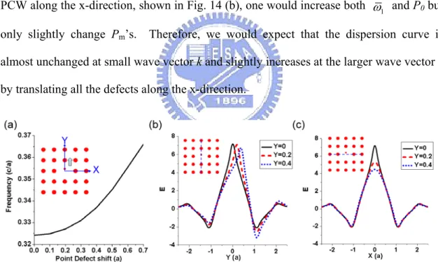
Fig 13 The eigenfrequencies, the electric field of the point-defect modes with a defect rod located at different positions………..………..36

Fig. 14 The ways of moving the defect rods in single or coupled PCWs………..37

Fig. 15 The electric field distribution of the point defect mode before and after moving the defect rods………..………..39 Fig. 16 Dispersion curves of a single PCW with all the defect rods moving along the

y-direction, and the x-direction………..………40 Fig. 17 The dispersion curves of the shifted directional couplers (DCs)………...41 Fig. 18 The dispersion curves as moving the defect rods along the x-direction…………42 Fig. 19 The dispersion relation curves and the FDTD simulation results of the original

DC without moving defects, longitudinally moving the defect rods by 0.5a, and transversely moving the defects closer by 0.5a………..……….43 Fig. 20 The electric field distribution of a point defect mode in the square lattice……...47 Fig. 21 Simulation results of asymmetric DCs by the PWEM ……….50 Fig. 22 The wave vectors, the mode amplitude ratio of the bonding (antibonding) mode,

List of Tables

Chapter 1 Introduction

1.1 Photonic crystals

Photonic crystals (PCs) arise from the cooperation of periodic scatters thus, they are called “crystal” because of their periodicity and “photonic” because of their action on light [1]. The concept behind these materials stems from pioneering work of Yablonovitch and John [2-6]. Yablonovitch proposed a structure in which an electronic and photonic gap overlapped, making it possible to enhance the performance of lasers, heterojunctions, bipolar transistors, and solar cells [4]. In the same year, John also proposed using such structures for the localization of light in strongly scattering dielectric structures [3]. A PC is interesting owing to whose band structure possesses a complete photonic band gap (PBG) [5-7]. A PBG defines a range of frequencies in which light cannot propagate inside the crystals. As a result of the existence of PBGs and their unusual dispersion properties, photonic crystals can sustain various light waves, pulses, and beam propagation regimes which are of physical interest and important for numerous applications, such as perfect reflector and negative refraction index structures.

The mathematic description of the PCs should start from the four Maxwell’s equations rather than other scalar wave description, such as the beam propagation method, because the special variation of the refraction index is comparable to the wavelength. From the researches in early 1990s, four main algorithms are proposed to model the wave propagation in the PCs. They are the plane wave expansion method (PWEM) [8, 9], finite difference time domain (FDTD) method [10-12], finite element method (FEM) [13, 14] and transfer matrix method (TMM) [15, 16]. The PWEM deals with the Maxwell’s

equations in wave vector space and solves the eigenfrequencies in each wave vector to get the dispersion relation. It is suitable for the high periodic structures. In the FDTD method, a wave propagating through the PC structure is found by a direct discretization of Maxwell’s equations in both time and space. It is powerful and flexible especially in a complex structure but is extremely time-consuming and its computational requirements grow exponentially with problem size. The FEM is a frequency domain method used to solve Maxwell’s equations. It takes into account material discontinuities in the dielectric structure more efficiently by a preconditioned subspace iteration algorithm, which helps overcome the slow convergence of the PWEM. It is widely used to simulate the dispersion of the photonic crystal fiber due to its structure uniformity in the wave propagation direction. TMM is powerful at layer structures such as 1D PCs or 2D and 3D PCs with square lattices. A matrix is used to connect the electric field or magnetic field between two layers. By solving the matrix, the transmission, refraction and dispersion relation can be obtained.

1.2 Photonic crystal waveguides and coupled resonant optical

waveguides

A photonic crystal waveguide (PCW) can be created by sequentially changing the radius or dielectric constant of the dielectric rods or changing the radius of periodic air holes in a dielectric slab; on the other hand, the coupled resonator optical waveguide (CROW) is created by arranging the cavities, made of point defects, periodically [17, 18]. The electromagnetic (EM) wave can propagate in these channels, PCWs or CROWs, with a very low loss even through a sharp bend [19]. Combining the point defects with the

PCWs or CROWs can be used to modulate the wave [20-22]. Lots of researches were focused on design the structures to modulate light to realize the all optical devices such as (1) Waveguide crossings: The perpendicular crossings in the waveguides intersection exhibit negligible crosstalk which closes to 10% when the waveguide width is on the order of a wavelength. The design in PC waveguide permitting single-mode waveguides with optimal miniaturization falls as low as 10-9 [23]. (2) Waveguide branches: An idea waveguide branches is a device that splits the input power into two or more output waveguides without significant reflection or radiation losses [24, 25]. (3) Channel drop filters: Channel dropping filters are devices that are necessary for the manipulation of wavelength division multiplexing optical communications [26]. PCs present a unique opportunity to investigate the possibilities of miniaturizing such a device to the scale of the wavelength of interest.

These defect resonators in the CROWs are designed such that their resonant frequency falls within the band gap of the surrounding 2D structure, which permits high-Q optical modes and the coupling is due to the overlap of evanescent waves between two cavities [17]. Therefore, the energy is strong localized in the cavities with very low group velocity. If nonlinear media are added in the cavities, the high Q and slow light in the CROWs will enhance the nonlinearity of the media. Another appearing feature of the CROW is the possibility of making lossless bends. Since the coupling of the corner resonator to its two immediate neighbors is identical due to its rotational symmetry, the transmission coefficient through the bend is 100% throughout the entire CROW band. That is contract with the PCWs, 100% transmission occurs only at a particular frequency [19].

1.3 Photonic crystal coupler

The photonic crystal coupler is formed by two adjacent PCWs with one or several row(s) of partition rods [27, 28]. When we calculate the dispersion relation of this structure of two identical PCWs, there would be two dispersion relation curves existed within the band gap [29, 30]. One is odd mode and the other is even mode [29]. An EM wave with a given frequency located on the dispersion curves is incident into one channel (PCW) of this coupler will couple into the other channel. The coupling length, in which the EM wave completely or maximally couples into the other waveguides for the symmetric or asymmetric cases, is defined as π/Δk, where Δk is the wave vector mismatch between two modes at the given frequency. The coupling length highly depends upon the incident frequency that can be used to design the demultiplexer [30-32]. The directional coupler can also be used to design power splitter [33], polarization splitter [34] and add/drop filters [35]. If a nonlinear medium is added in the branch of the waveguides, the switch which is controlled by the EM wave or the external electric field can also be fabricated by directional coupler structures [36].

1.4 Motivations

The tight binding theory (TBT) has been widely used in the CROWs to describe the amplitude of the EM wave propagation in linear or nonlinear system. When a plane wave is incident in these structures, the dispersion of the CROWs can be obtained by PWEM. The numbers of the separation rods extremely influence the sign and the slope of dispersion relation. From the dispersion relation, we can derive the group velocity and various orders of the group velocity dispersion (GVD) which means the difference of the separation rods in the CROWs will also determine the sign and the magnitudes of the

group velocity and GVD. Once, the nonlinear material is added in the waveguides region, the dispersion relation curve of the CROW has a constant frequency shift comparing to the curve of linear waveguides, so the linearly physical properties of the waveguides will be preserved and the properties will influence the performance of the nonlinear materials. Therefore, the properties of the CROWs with different separation rods or structures should initially be investigated and the TBT provides a powerful method for us to realize these properties.

As the defect rods are made of nonlinear materials such as Kerr media, the perturbation superimposed on a plane wave could grow exponentially at a certain condition. It is named as the modulation instability (MI). Because the field evolution in the PCWs with Kerr media can be expressed as a discrete nonlinear Schrödinger (DNLS) equation, the MI region and gain can be derived from this equation. On the other hand, when a pulse is incident into the waveguides with nonlinear materials, the pulse could propagate in the waveguides without distortion which is the so-called soliton. The criterion for soliton propagation under slowly varying envelope approximation (SVEA) can also be derived by the DNLS equation. Therefore, we can use this criterion to discuss the soliton propagation regions in different structures of CROWs. When the width of the pulse becomes shorter, the SVEA is broken. The soliton disperses under propagation due to the high order GVD. We can take the Fourier transform of the amplitudes of the pulse to discuss the pulse broadening caused by high order GVD under soliton propagation condition.

In PCWs, the distance between two defect rods (a) is so close that the next nearest-neighbor coupling is no longer negligible. Under this circumstance, the evolution equation to describe the wave propagation in the PCWs with nonlinear material

should be written as an extended formula. In general, the next nearest-neighbor coupling coefficient is approximately one order smaller than the nearest-neighbor coupling coefficient, such making the properties in the PCWs is different from the properties in the CROWs especially when ka = π/2. Therefore, it is needed to take advanced discussion on the MI and soliton propagation in the PCWs.

When the other identical waveguide is carved into PCs and partitioned with one or several rows of perfect rod(s), another useful device, the directional coupler (DC), is created. The dispersion relation curve of the coupler is usually crossing with triangular lattice but rare crossing in the square lattice. This phenomenon gives some limitation as designing the device. Therefore, we want to create the crossing point in the square lattice and then to move the crossing point at square lattice or triangular lattice which be achieved by moving the defect rods in the waveguides. We also want to use TBT to further realize the trend of shift of the crossing point as moving the defect rods.

On the other hand, when the other waveguide is created asymmetrically, the dispersion relation calculated by PWEM would not cross anymore, but the parity of the eigen mode may switch at a particular point, in which point we named it the decoupling point. At this point, the electric field is only localized at one waveguide of this asymmetric coupler. These phenomena cannot give a good explanation by the numerical simulation results. Therefore, we also want to use TBT to derive an analytic description to realize the physical properties of asymmetric PC couplers.

1.5 Organization of the dissertation

In this dissertation, we firstly use TBT to derive the electric field evolution equation in single PCWs and CROWs with or without the nonlinear media in Chapter two. The

coupling equations of double PCWs and the properties are also discussed in this chapter. By using the derived equation, we discuss the MI when the Kerr media are added in the PCWs or CROWs in Chapter 3. In the Chapter 4, the soliton propagation criterion and pulse broadening at this criterion is discussed. We found the soliton propagation regions agree with those of the MI. In Chapter 5, we investigate the mechanism which causes the movement of the crossing point of the dispersion relation curves by TBT. In Chapter 6, the coupling equations of asymmetric PC coupler are derived to discuss mode switching phenomena and the simulation results by the PWEM.

Chapter 2 Tight binding theory

2.1 Photonic crystal waveguides and coupled resonant optical

waveguides

We consider an optical waveguide which consists of a periodic sequence of identical single-mode defects in the PC with lattice constant aL as shown in Fig. 1. The distance

between successive defect points or cavities is a. Assuming the isolated point defect is a single mode with eigenfrequency of ω0 and electric field distribution in triangular and

square lattices as shown in Fig. 2, we can express the electric and magnetic fields of each point defect as E(r,t) = E0(r)exp(-iω0t) and H(r,t) = H0(r)exp(-iω0t). Let us assume that

the presence of the other defects near a particular site perturbs the total permittivity from

ε(r) to ε'(r). The fields in the waveguide 0

0 ( , )_t ( , )_{t e}−iωt ′ = ′ E r E r and 0 0 ( , )_t ( , )_{t e}−iωt ′ = ′

H r H r should obey the equations: ∇ ×E0′ =μ ω0(i 0H′0 − ∂H0′ / )∂t and

0 0 0

(i / )t

ε ω

′ ′ ′ ′

∇ ×H = E − ∂E ∂ .

Using the divergence theory of ∇ ⋅(E*0×H0' +E'0×H*0), we can get the Lorentz

reciprocity relation [37]: * ' ' * * ' * ' * ' 0 0 0 0 0 0 0 0 0 0 0 0 ( ) ( / / ) d × + × = dv iω εΔ ⋅ −ε′ ⋅ ∂ ∂ −t μ ⋅ ∂ ∂t

∫

s E H E H

∫

E E E E H H (2.1)

with Δε=ε-ε’. The electric field E r0′( , )t and magnetic field H′0( , )r t of the

waveguide can be expressed as a superposition of the bound states, i.e.,

0( , )t b tm( ) 0m

′ = ∑ ′

E r E and H r0′( , )t =

∑

b tm′( )H0m , where E0m =E r0( −ma) and 0m = 0( −ma).

0 ( ) ( ) i t m m b t =b t e′ −ω , we obtain n ( 0 0) n m( n m n m) 0. m db i P b P b b dt + −ω + +

∑

+ + − = (2.2)

Here the coupling coefficient Pm is defined as

0 0 0 2 2 0 0 0 ( ) n n m m n n d E E P d H E ω υ ε υ μ ε + Δ ⋅ = ⋅ +

∫∫∫

∫∫∫

(2.3)

P0 is a small shift arising from the presence of the neighboring defects. When we

consider a plane wave with wave vector k and frequency ω is incident into this waveguide, the dispersion of the waveguide becomes

0 0 1 1 ( ) 2 cos( ). m ka P P ka ω ω = = − −

∑

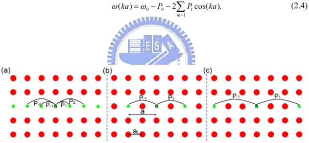
(2.4)

Fig. 1 The structures of (a) a PCW, (b) a CROW with one separation rod and (c) a CROW with two separation rods, where a is the length of successive defect points and aL is the lattice constant

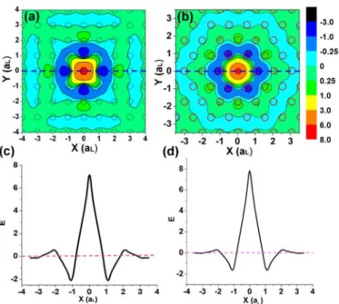
Fig. 2 The electric field distribution (Ez) of a point defect in square lattice for (a) f = 0.364 c/aL

with reduce rod ( rd = 0.05aL) defect and (b) f = 0.333 c/a with rd=0.1aL. (c) (d) The electric field

distribution of the blue dash line in (a) (b).

2.2 The properties of coupling coefficients in PCWs and CROWs

The electric field distribution (Ez) of a single point defect, simulated by the PWEM in

the square lattice and triangular lattice with the dielectric constant and radii of dielectric rods being 12, 0.2aL is shown in Fig. 2. The radius (rd) of the defect rods and eigen

frequency in square lattice are 0.05aL and 0.364 c/aL; those in triangular lattice are 0.1aL

and 0.333 c/aL. The field profile along the (blue) dash line in Fig. 2(c) and (d) has the

opposite sign when extending to odd nearest-neighbor rod(s) (E0(0,0)*E0(xa,0) < 0, x =

1,3,5,…) and has identical sign when extending to even nearest-neighbor rods [18, 38]. To maintain a single mode propagating in the waveguides, the radius or the refraction index of the rods in the waveguides is reduced therefore Δε is negative in the following discussion. Since the electric field is mainly localized around the dielectric rods of the waveguides, we can use the maximum values to replace the integral values for a simple

estimation of Eq. (2.3). Therefore, P1 is positive in even-separated-rod CROWs, in

which E0(0,0)*E0(xa,0) < 0, x = 1,3; P1 is negative in odd-separated-rod CROWs; | P2 | is

two orders smaller than | P1 | so P2 is negligible for considering the dispersion relation.

In the PCWs, P1 and P3 are positive and P2 and P4 are negative; P3 is two orders of

magnitude smaller than P1, and thus only P1 and P2 need to take into consideration when

calculating the dispersion relation. From the dispersion relation in Eq. (2.4), the frequency increases as k increases in PCWs and CROWs with even separation rods where

P1 is positive, but the frequency decreases as k increases in the CROWs with odd

separation rods.

2.3 Discrete nonlinear Schrödinger equation

If a Kerr medium (n2 =n02+2n n0 2 E2) is added around the defects, Eq. (2.2) can be

written as a DNLS equation [37]: 2 0 0 ( ) ( ) 0. n n m n m n m n n m db i P b P b b b b dt + −ω + +

∑

+ + − +γ = (2.5)

The self phase modulation (SPM) strength is

4 0 2 0 0 0 2 2 0 0 0 2 ( ) n n n n n d E d H E ε ω υ γ υ μ ε = +

∫∫∫

∫∫∫

(2.6) with n2 being the Kerr coefficient. Let the plane wave with amplitude φ, propagation

wave vector k, and frequency ω in site n as bn = φexp(inka-iωt) being the solution of Eq.

(2.5). The dispersion relation of the nonlinear PCW can be derived as

2 2

0 0 1 2

( )ka c 2 cos( ) 2 cos(2 )c ka c ka | | | | .

ω =ω − − − −γ φ =ω γ φ′− (2.7)

Here, ω’ is the dispersion relation of linear waveguides. The SPM will make the dispersion relation a constant frequency shift in all wave vectors. The positive Kerr

coefficient leads a low frequency shift and vice versa.

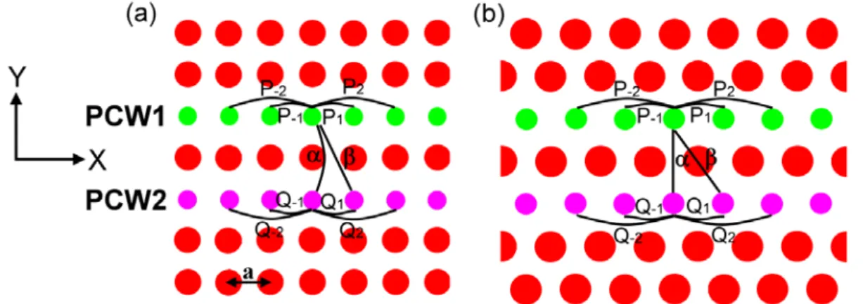
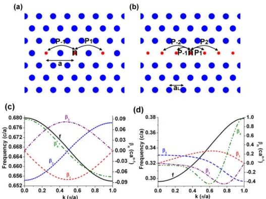
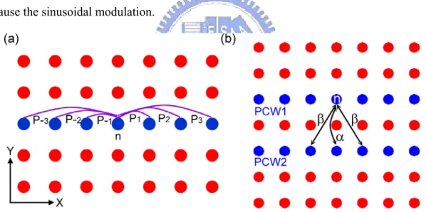
Fig. 3 Geometric structures of the photonic crystal waveguide couplers of (a) square lattice and (b) triangular lattice with the lattice constant a. Ps and Qs are the coupling coefficients between defects within a single waveguide. α, and β are the coupling coefficients between waveguides.

2.4 Coupling equations in asymmetric photonic-crystal coupler

We consider an asymmetric coupled PCWs in a PC with the lattice constant a, in which

a = aL, are formed by two rows of periodic defect rods partitioned by a perfect row of rods,

shown as PCW1 and PCW2 in Fig. 3 for the square and the triangular lattices, respectively. The field distribution of the eigenmode of an isolated (point) defect in each PCW can be written as the product of time-varying and spatial-varying functions, i.e., E10(r,t) = u0(t)E10(r) in PCW1 and E20(r,t) = v0(t)E20(r) in PCW2, where

u0(t)=U’exp(-iω1t) and v0(t)= V’exp(-iω2t), with U’ and V’ being the constant amplitudes

of electric fields and ω1 and ω2 the frequencies of localized modes of the point defect in

each PCW.

Under the TBT, the evolution equation of the isolated PCW1 can be written as

1 0 1 ( ) ( ) n n m n m n m m i u P u P u u t ω ₌ + − ∂ _{= − − +} ∂

∑

(2.8)

and 11

m m

P =P , where ij m

P is the coupling coefficient between the site n of the ith PCW and the site n+m of the jth PCW, and is defined as

2 2 0 ( ) . [ ] i in jn m ij m in in dv P dv ω ε μ ε ∞ + −∞ ∞ −∞ Δ ⋅ = +

∫

∫

r E E H E (2.9) Let k and ω be the wavevector and its corresponding eigenfrequency of PCW1,₁ respectively, we obtain the dispersion relation of PCW1:

1 1 0 1 ( ) 2 _mcos( ). m k P P mka ω ω = = − −

∑

(2.10) Similarly, the evolution equation and dispersion relation of the isolated PCW2 are shown below: 2 0 1 ( ) ( ), n n m n m n m m i v Q v Q v v t ω ₌ + − ∂ = − − + ∂

∑

(2.11) 2 2 0 1 ( ) 2 _mcos( ), m k Q Q mka ω ω = = − −

∑

(2.12) where 22 m m

Q =C , vn(t) and ω are the time-varying function and the eigenfrequency of 2

the isolated PCW2, respectively.

Due to the field distributions of defect modes being not strongly localized around defects, we shall consider the coupling effect of two asymmetric PCWs up to the second nearest-neighboring defects, with coupling coefficient 12 21

0 0 C C α= = and 12 21 1 1 C C

β= ± = ± shown in Fig. 3 for the square and the triangular lattices, respectively.

The coupled equations of asymmetric PCWs are given by [39, 40]:

_{1 0 1 1} 1 ( ) ( ) ( ), n n m n m n m n n n m i u P u P u u v v v t ω ₌ + − α β + − ∂ _{= − − + − − +} ∂

∑

(2.13) 2 0 1 1 1 ( ) ( ) ( ). n n m n m n m n n n m i v Q v Q v v u u u t ω ₌ + − α β + − ∂ _{= − − + − − +} ∂

∑

(2.14)

When the stationary solutions of coupled Eqs. (2.13) and (2.14) are taken as un = U0

exp(ikna-iωt) and vn = V0 exp(ikna-iω t), we obtain the characteristic equations of the

coupler:

1 0 0

(ω ω− ) U +g ka V( ) =0, (2.15)

2 0 0

(ω ω− ) V +g ka U( ) =0, (2.16) where g ka( )= +α 2βCos ka( ) and 0

0 U

V

⎡ ⎤ ⎢ ⎥

⎣ ⎦ stands for the eigenvector or field amplitudes in

two PCWs. The eigenfrequencies (dispersion relations) and eigenvectors (field amplitudes) of Eqs. (2.15) and (2.16) are

1 2 2 2 ( ) ( ) ( ( )) , 2 k ω ω g ka ω± ₌ + _{± Δ + (2.17)} 2 2 0 0 ( ( )) ( / ) , ( ) g ka V U g ka χ± ₌ ± _{= −}Δ ± Δ + _(2.18)

where Δ =(ω₂−ω₁) / 2 and χ± _{are the amplitude ratios corresponding to frequencies}

( )k

ω± _{. Note that χ χ}+ − _{= −1 is due to the orthogonality of these two eigenmodes at a}

given wave vector k. At a given frequency, χ χ+ − _{is not necessarily equal to -1. In}

symmetric waveguides,ω₂=ω₁, Eqs. (2.17) and (2.18) will become [41]

1 ( )k g ka( ), ω± ₌ω _{± (2.19)} 0 0 ( /V U ) 1. χ± ₌ ± _{= ± (2.20)}

The existence of g(ka) makes the eigenstates of the coupler be the linear combination of eigenstates of the single waveguides, leading the EM wave coupled from one waveguide from another. When g = 0, the waveguides will be no longer coupled to each other that means the coupling length is infinite.

In this chapter, we used TBT to derive the coupling equations to describe the electric field propagation in nonlinear or linear single waveguides and linear symmetric or asymmetric PC couplers. In the following chapters, these equations will be used to

further discuss pulse propagation in the PCWs and CROWs with nonlinear media and the EM wave coupling between two waveguides.

Chapter 3 Modulation instability in a single PCW and CROW

3.1 Introduction

A pulse experiences serious dispersion in the PCWs and CROWs [42, 43]; therefore, it would hardly propagate within the waveguides without broadening. There are two ideas to improve the situation of allowing the pulse propagation in the waveguides without broadening. The first method is to design a proper structure to create a linear dispersion curve in the range of operating frequency to provide dispersionless propagation; the other method is to add nonlinear Kerr media to provide soliton propagation [37, 44-46].

However, in the latter case, the criteria of forming a soliton is that the wavevector of the incident wave must be located within the modulation instability (MI) regions [46-48], where the MI refers to a process in which a small perturbation upon a uniform intensity beam would grow exponentially [49]. This phenomenon, which is commonly observed in nonlinear optical fibers [50], will also occur in the nonlinear PCWs and CROWs.

3.2 Modulation instability gain

In Section 2.3, we have derived the DNLS equation to describe the EM wave propagating in PCW or CROWs. Now, considering a small perturbation νn(t)

superimposed on a plane wave with wave vector and frequency being p and ω, shown as [49]

( )

( ( )) i pna t ,

n n

b _{= φ+}v t e −ω _(3.1)

we can substitute Eq. (3.1) into Eq. (2.5) in which the 1st _{and the 2}nd _{nearest-neighbor}

1 1 1 2 _* 2 2 2 ( 2cos( ) ) ( 2cos(2 ) ) ( ) 0. n ipa ipa n n n ipa ipa n n n n n dv i P v e v e pa v dt P v e v e pa v γ φ v v − + − − + − + + − + + − + + = (3.2)

Taking νn(t)as this form [49]

*

1 2

( ) ( iqna iqna) i t,

n t V e V e e

ν

_{= +} − − Ω _(3.3)

where q and ω are the wavevector and frequency of the modulation perturbation, V1 and

V2* represent small perturbation with perturbation wavevectors of q and – q, and

substituting vn(t) into Eq. (3.2), we obtained the dispersion relation of the perturbation:

2 ( , )p q B A A( γ φ| | ) Ω = ± − (3.4) with 2 2 1 2

4 cos( )sin ( ) 4 cos(2 )sin ( ) 2

qa

A= P pa + P pa qa (3.5) and

1 2

2 sin( ) cos( ) 2 sin(2 ) cos(2 )

B= P pa qa + P pa qa . (3.6) If the dispersion relation Ω (p,q) is complex as A(A - γ|φ|2) < 0, the perturbation field

would become unstable. The intensity growing rate G of MI, also called the MI gain, is related to the imaginary part of Ω (p, q) by

G(p,q)=2*Im(Ω (p, q)) =

1

2 ₂ 2 _{2 2} 4

Re(2⋅A(γ φ −A) ) 2 Re= ⋅ − −(A 0.5γ φ ) +0.25γ φ . (3.7)

3.3 Gain regions and profiles analysis

Because of P2 ≈ 0 for the CROWs, the coefficient A can be rewritten as

2 1

4 cos( )sin ( / 2)

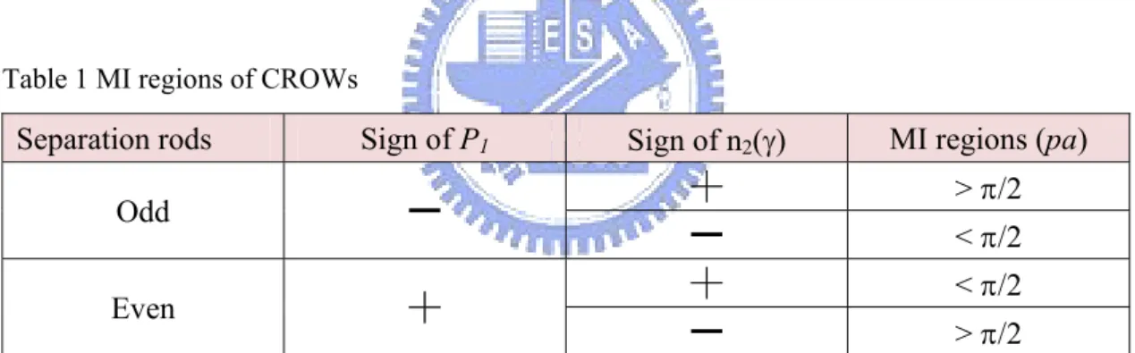
A= P pa qa , in which the sign of A is determined only by pa and it changes sign at pa = π/2. Here the region of pa (or qa) is defined between 0 and π. For positive (negative) A, γ must also be positive (negative) and γ|φ|2 _{> A > 0 (γ|φ|}2 _{< A < 0) to support}

MI, which can be easily derived from Eq. (3.7); in other words, P1cos(pa)γ must be

positive in MI region. Therefore, the boundary of MI must be located at pa = π/2. In odd-separation-rod CROWs, P1 is negative, therefore A and γ must be both negative when

0 < pa < π/2 and positive as pa > π/2. However, in even-separation-rod CROWs, P1 is

positive, therefore A and γ must be both positive when 0 < pa < π/2 and negative as pa > π/2, shown in Table 1. When the structure of the waveguide (P1) has been chosen, |A|

increases if q increases at constant P1 and p. When we plot the gain profile as the graph

of G vs. q at a given p and define the gain maximum as the maximal values in the graph, from Eq. (3.7), the gain maximum would be located at A = 0.5γ|φ|2 and cut off at A = γ|φ|2

when 2

1

4 |Pcos(pa) | 0.5 | |> γ φ ; otherwise, the gain maximum would be located at qa = π.

Table 1 MI regions of CROWs

Separation rods Sign of P1 Sign of n2(γ) MI regions (pa)

Odd ━ ┼ > π/2

━ < π/2

Even ┼ ┼ < π/2

━ > π/2

In negative (positive) P1 for an odd-separation-rod (even-separation-rod) case, the

slope of dispersion relation is negative (positive) [51] and the frequency dispersion β2

defined as d2ω/dk2 _{is negative (positive) when pa < π/2 and positive (negative) for pa >}

π/2 from Eq. (2.4). Therefore, for negative β2 (pa < π/2 for the odd-separation-rod case

and pa > π/2 for the even-separation-rod case), the negative γ is needed to support MI and positive γ is needed to support MI for positive β2. In other words, the MI regions of the

In PCWs, P1is positive and P2, which cannot be neglected, is negative. First, we

consider the positive Kerr media having positive n2 (or γ) so the criterion of the MI is γ|φ|2

> A > 0. From the criterion of A=4 cos(P1 pa)sin (2 qa/ 2) 4 cos(2 )sin ( )+ P2 pa 2 qa > 0,

since P2is an order of magnitude smaller than P1, this criterion can be further reduced to

cos(pa) > -4| P2 / P1 | cos2(qa/2). Under this circumstance, the MI region is determined

not only by pa but also by qa, and pa in the MI region can exceed π/2, unlike in CROWs that the MI boundary for pa is located at π/2 and is independent of qa. From the other criterion: γ|φ|2 > A, we found A is dominated by the P1 term as pa is located away from

π/2, in this case the MI gain is similar to that in the CROWs with even separation rods. Contrarily, when pa approaches to π/2, the P1 term is almost zero and A becomes

dominated by the P2 term. In this case, A would not increase as increasing qa. From

Eq. (3.7), we knew that the maximum of the gain profile, G(q), is located at A = 0.5γ|φ|2

or dA/dq = 0. For the latter case, the peak gain would be smaller than that of the former condition. When 4P2 cos(2pa) < 0.5γ|φ|2, there would be two gain maxima at a fixed pa

and the gain maxima is located at A = 0.5γ|φ|2, but there would be only one gain maximum located at dA/dq = 0 as 4P2 cos(2pa) < 0.5γ|φ|2.

On the other hand, in the condition of negative γ, the first criterion is cos(pa) < -4 | P2

/ P1| cos2(qa/2). We found the MI would happen only when pa > π/a. However, when

0 > cos(pa) > -4|P2 /P1|, the MI region is located at the higher q rather than the general

case in which the perturbation would have gain at qa = 0+. The cutoff gain is also decided by A = γ|φ|2.

We consider a square lattice PC with the dielectric constant and radii of the dielectric rods being 12 and 0.2aL, where aL is the lattice constant of the PCs. The radii (rd) of the

defect rods are reduced to be 0.05aL and the Kerr media are introduced around the defects

between one separation rod to create the CROW and sequentially to create the PCW. The structures and dispersion relations of the CROW and PCW in TM polarization (the electric field parallels the rod axis) without Kerr media are shown in Fig. 4, which are simulated by the PWEM.

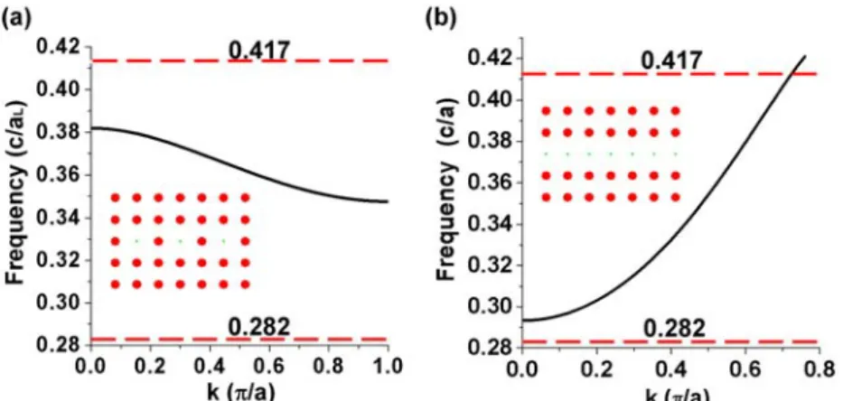
Fig. 4 The dispersion relations of (a) a CROW with one separation rod and (b) a PCW in square lattices, which are simulated by the plane wave expansion method. The dash red lines are the edges of the band gaps.

Fig. 5 (a) The values of A and (b) the gains and regions of the MI of the CROW with γ|φ|2_=0.01

First, the properties of the MI in the CROW would be discussed. The coupling coefficient P1 is -0.00841 (2πc/aL), where c is the speed of light in the vacuum. Because

P1 is negative, the eigenfrequencies will decrease as increasing k. Figure 5(a) shows A

vs. qa with different p. Let A’ = γ|φ0|2－A so that G = 2 AA′ . As aforementioned, the

MI region is determined by the condition that A lies between 0 and γ|φ|2 _{and the}

maximum of G appears when A equals (or is the closest) to 0.5γ|φ|2. Figure 5(b) shows G(p,a) with γ|φ|2=0.01 (2πc/aL). It can be seen that there is no MI gain when pa ≤ 0.5π

and only a single gain maximum at given pa in the condition of pa > 0.576π.

In PCWs, the coupling coefficients of P1 and P2 are 0.039 and -0.0047(2πc/a), and ω0-

P0 is 0.3632 (2πc/a). The values of A at a given pa were shown in Fig. 6(a). When pa

is small, i.e., in [0, 0.4π], A is dominated by P1 term and A increases as qa increases.

Due to P1 is positive, the properties of MI would be similar to the CROWs with even

separation rods that possesses a single gain maximum as the solid curve in Fig. 7(a) for pa = 0.4π. However, as pa is in (0.4π, 0.6π], A is not simple increasing or decreasing function of qa, shown in Fig. 6(b). At a given pa with positive Kerr media (γ > 0), when the values of A(q) is always smaller than 0.5γ|φ|2, e.g., γ|φ|2 = 0.01 (2πc/a) _{and pa = 0.6π,} there would be a maximal gain as the solid curve in Fig. 7(d). However, when A(q) is larger than 0.5γ|φ|2_{, e.g., γ|φ|}2_{=0.01 (2πc/a) and pa = 0.49π and 0.55π, there would have 2}

gain maxima, solid curves shown in Figs. 7(b) and (c). And the MI region with positive γ can extend to pa = 0.6π, as shown in Fig. 6(c). On the other hand, the MI region with negative Kerr media is shown in Fig. 6(d) which is located within π/2 < pa < π but having the MI region located at high qa as pa close to π/2.

Fig. 6 (a) (b)The values of A in the PCW. The region and gains of MI with (c) positive Kerr media (γ |φ |2_{=0.01*2πc/a) and (d) negative Kerr media (γ|φ |}2_{=-0.01*2πc/a).}

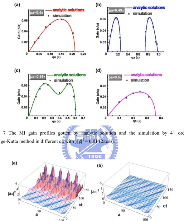
Next, we would use the 4th order Runge-Kutta method to simulate the evolution of the perturbation. A plane wave with 10% initial sinusoidal perturbation is used as the input source in a square-array PCW with γ|φ|2 = 0.01 (2πc/a). The perturbation will grow exponentially in the MI region to become a discrete soliton before it splits, as shown in Fig. 8(a), but the perturbation would never grow outside the MI region Fig. 8(b). We plot the gain coefficients with square dots in Fig. 7 by evaluating the growing rate by the Runge-Kutta method then compare with gain profiles (solid curves) calculated by using Eq. (3.7). The results show a quite good agreement.

Fig. 7 The MI gain profiles gotten by analytic solution and the simulation by 4th _order

Runge-Kutta method in different qa with γ|φ|2 _{= 0.01 (2πc/a).}

Fig. 8 The evolution of the perturbation in the PCW with (a) pa=0.4π and qa=0.1π (b) pa=0.6π and qa=0.1π.

3.5 Summary

We have successfully used the TBT to investigate the MI in both CROWs and PCWs by considering growth of a small perturbation superimposed on a plane wave. The

number of separation rods in the CROWs would decide the signs of the nearest-neighbor coupling coefficients (P1) and the next nearest-neighbor coefficient (P2) can be neglected

because it is more than 2 orders of magnitude smaller than P1. This leads to positive

dispersion for a positive coupling coefficient and vice versa. Although the signs of the coupling coefficient could be different, the criterion: P1cos(pa)γ > 0 for obtaining MI is

the same for incident plane wave of wave vector p. Therefore, the MI region can only be located in either pa < π/2 or pa > π/2 with only one gain maximum. In the air-defect PCWs, P1 is positive and P2, which is no longer negligible, is negative. It makes the MI

gain of positive Kerr media located at low wavevectors and vice versus. The boundary of gain region of pa is not exactly at π/2 due to the MI is mainly dominated by P2 term as pa

approaches π/2 and there could exist two gain maxima. Furthermore, the numerical simulation using the 4th order Runge-Kutta method reveals exponentially growing perturbation intensity as it propagates and the growing rate matches with the gain coefficient of MI in the analytic solution.

In next chapter, a pulse will be incident into the waveguide within or without the MI region to understand if a soliton can exist in the MI region. At the same time, the soliton propagation criterion will also be derived to observe the soliton propagation under this criterion.

Chapter 4 Soliton propagation in a single PCW and CROW

The amplitude evolution of the electric field in the nonlinear CROWs containing Kerr media often leads to DNLS equation derived by the TBT [37, 51-53] and Section 2-3. By solving the DNLS equation under long-wavelength approximation, this equation reduces to a nonlinear Schrödinger (NLS) equation. Spatiotemporal discrete solitons can propagate undistorted along the defects by balancing the effects of discrete lattice dispersion with material nonlinearity [37]. However, as the pulse becomes narrow, the long-wavelength approximation will be broken and high order dispersions should be considered [53]. Therefore, the more generalized criteria for solitons propagation in different structures of CROWs [51], e.g., different numbers of separation rods between two cavities or different pulse widths, should be derived. Moreover, in the PCWs, the defect rods are so close that the next nearest-neighbor coupling cannot be neglected [41]. The governed equation of motion is termed the extended discrete nonlinear Schrödinger (EDNLS) equation to distinguish the equations in CROWs in which only the nearest-neighbor coupling coefficient is considered. There are rare reports on pulse propagation in nonlinear PCWs using the TBT but the Green-function approach[44, 45]. Although the equations obtained from these two approaches are quite similar [54], it still lacks on the research about the dynamic or criteria of soliton propagation in the PCWs. Therefore, it is needed to take the advanced discussion about criteria of solitons propagation of different kinds of CROWs or PCWs, and to derive the EDNLS evolution equation for describing the dynamic properties of solitons with different nonlinear strengths and pulse widths.

4.1 Soliton propagation criteria

In order to get the soliton solution and to give the advanced analysis of high-order dispersion as pulse propagating, we let x = na and i kx( t)_.

n

b ₌φe −ω′ _{Taking the Taylor’}

expansion of φ [53] 1 ( ) , ! = ∂ + = + ∂

∑

n nn n a x a n x φ φ φ (4.1) Eq. (2.5) can be written as a NLS equation:

2 1 ( ) | | 0. ! = ∂ ₋ − ∂ _{+ =} ∂

∑

∂ n n n n n i i t n x φ _β φ _{γ φ φ (4.2)}

The dispersion coefficients, βn, equal to ∂nω( ) /k ∂kn or

2 1 1 2 1 2 1 1 2 − ( 1) + − sin( ), − = = n − n

∑

n n m m a m P mka β (4.3) 2 1 2 2 1 2 ( 1) + cos( ). = = n − n

∑

n n m m a m P mka β (4.4) Therefore, the angular frequency of the waveguides can also be expressed as the Taylor’ expansion sum of dispersion coefficients, i.e.,

2 3

0 1 2 3

( )k = + Δ +k (Δk) / 2!+ (Δk) / 3!+ ⋅⋅⋅,

ω ω β β β (4.5)

where β1 is the group velocity (vg) of the solitons in these waveguides if the high-order

terms is neglected. When the variation of the pulse amplitude is smooth enough, i.e., (Δ ) / ! 0n ≈ n k n β or ∂ ≈0 ∂ n n n x φ

β for n > 2, Eq. (4.2) has a soliton solution as

1 ( ) 0

sech(

−

)

−

.

=

x

t

i kx t

b

e

x

ω

β

φ

(4.6) The criterion to support a soliton propagation is thus 2 2

0 = 2/x0

γφ β or

2 2 2

1 2 3 0

=2 ( cos(a P ka) 4+ P cos(2ka) 9 cos(3 )+ P ka + ⋅⋅⋅) /x .

γφ (4.7)

into the nonlinear waveguides. The relationship between x0 and φ0 is determined by β2

and γ (n2 or χ(3)). The sign of β2 and γ must be the same to support a soliton

propagation and SPM strength (γs) is β2/(x02 2φ ).

In the CROWs, P2 is two orders of magnitude smaller than P1, so P2 can be neglected

in considering β2 and the soliton propagation criterion (SPC) in Eq. (4.7) can be further

reduced to 2 2 2

0 / =2 cos(1 ) /( ).

x a P ka γφ In even separated rods, P1 is positive so γ

should be positive at the SPC when ka < π/2 and γ should be negative as ka > π/2; however, in odd separated rod(s), P1 is negative so γ should be negative (positive) at the

SPC when ka <π/2 (ka > π /2), which correspond to the MI in these nonlinear waveguides [38] and the Kerr media should switch their signs when ka crosses π/2. In PCWs, P1 is

positive and P2 is negative with its value being an order of magnitude smaller than P1 [23].

Therefore, positive Kerr media should be put in the waveguides as a low wave vector or low frequency EM wave is incident, and vice versa. When the coupling coefficients Pn

(n > 2) are neglected for a simply estimation, Eq. (4.7) can be written as cos(ka) = -4 | P2 /

P1 | if γ = 0. Therefore, the border of switching sign of Kerr medium for soliton

propagation in PCWs occurs at ka > π/2. However, if the dielectric defect is used, in which Δε > 0, the signs of P’s should be changed and the type of Kerr media would also be changed accordingly.

4.2 Pulse broadening due to the high-order effect

To estimate the influence of high-order dispersion which makes the pulse broadening, and the width of the soliton pulse that can make the high-order term negligible, we took

the Fourier transform of the soliton solution, sech(x/x0), and calculated the standard

deviation of k’s distribution as Δk = 1/x0. Taking derivative of Eq. (4.5) with respect to k,

the group velocity can be expressed as

2 3

1 2 3 4

/ ( ) ( ) / 2! ( ) / 3! .

∂ω ∂ =k β +β Δ +k β Δk +β Δk + ⋅⋅⋅ (4.8) When the dispersion of β2 is balanced by the SPM and x0 > a, the pulse broaden will

mainly dominated by the lowest nonzero dispersion coefficients, βn, having n > 2. As

the GVD arises from β3 is determined by 0.5β3Δk2 and is proportional to (1/x0)2. The

dispersion can be neglected when 0.5β3Δk2t ≈ 0. At a particular frequency in which β3 =

0, Eq. (4.5) can be rewritten as

2 2

0 1 2( ) / 2!(1 ( 4/ 2) / 6)) .

= + Δ +k Δk + Δk + ⋅⋅⋅

ω ω β β β β (4.9)

From the dispersion relation in Eq. (2.7), the signs of β2 and β4 are opposite in all

propagation frequency of the CROWs and in mostly propagation frequency of the PCWs. Therefore, the term of (1+β4 / β2 Δk2/6) will be smaller than or equal to 1. We should

reduce the SPM strength (γs) to prevent overall SPM strength from making the pulse

narrowing, especially when the pulse width is short for large β4 and small (or zero) β3 at

ka approaches 0 or π. However, when the pulse is seriously dispersed in the waveguide, it is no longer having the form of hyperbolic secant (HS), the dispersion would be dominated by the β2 term again.

4.3 Simulation results and discussion

We consider triangular-lattice PCs with the dielectric constant and radius of the dielectric rods being 12 and 0.2aL. The radius (rd) of the defect rods is reduced to 0.1aL

CROW and sequentially to create the PCW as shown in Figs. 9(a) and (b). The dispersion curves, which were simulated by the PWEM, and dispersion coefficients (βn)

of the CROW and PCW in TM polarization without Kerr media are shown in Figs. 9(c) and (d). The coupling coefficient of P1 is -0.00652 (2πc/a) in the CROWs and P1, P2

and P3 are 0.02041, -0.00205 and 0.00026 (2πc/a) in the PCWs.

Fig. 9 (a) The structure of a CROW with a separation rod and (b) of a PCW in triangular lattice. The dispersion relations and dispersion coefficients of (c) a CROW with one separation rod and (d) a PCW in triangular lattices calculated by the plane wave expansion method.

Due to the magnitude of the coupling coefficients in the CROW is smaller than those in the PCW, the magnitude of the group velocity (β1) and the higher dispersion coefficients (β2,3,4) in CROWs would be smaller than in PCWs. However, because the signs of P1’s are different so that the EM waves in these two structures will propagate in

of β3 is almost symmetric at ka = π/2, leading to soliton propagations at k and 1-k (in π/a

unit) would be similar if different signs of Kerr media were introduced in the defects. However, it would behave quite differently in the PCWs. The border of switching sign of Kerr medium for soliton propagation occurs at ka > π/2, and the high-order dispersion coefficients (β3 ,β4) in high k is larger than those in low k due to the negligible 2nd and 3rd

next-neighbor coupling coefficients.

We will use the 4th _{order Runge-Kutta method to solve Eq. (2.5) to simulate an initial}

HS pulse propagating in the PCW and CROWs, because the HS pulse is a soliton solution. The advantage of using this method is to directly solve Eq. (2.5) without the requirement of calculating the dispersion coefficients. However, when the split-step Fourier method [53, 55] is used to solve Eq. (4.2), all orders of the dispersion coefficients are required to take into consideration for short pulse. On the other hand, if a Gaussian pulse is incident into the nonlinear waveguides with the same energy of the HS pulse at the SPC with small high-order GVD, the Gaussian pulse will initially develop into HS envelope, then finally the pulse becomes broadened due to the high-order dispersions that behaves like initially launching the HS pulse into the nonlinear waveguides.

4.3.1 Soliton propagation in the coupled resonant optical waveguides

To observe the pulse broadening without Kerr media or under the SPC, where

2 2 2

1 0

=2 cos( ) /( )

s c a ka x

γ φ in the CROWs with one separation rod and γs (n2) is positive

as ka > π / 2, we sent a hyperbolic-secant (HS) wave, i.e., φsech(x/x0)eikx with x0 = 2a

into the CROWs and let it propagate 400a/c in different k’s as shown in Fig. 10. It can be seen that the pulse would spread seriously without Kerr medium but spread slightly or

even preserve at the SPC. Because β2 = 0 at ka = 0.5π, the pulse would not spread even

without Kerr medium, whereas, the dispersive waves were observed at the farther distance wing with the larger x in Fig. 10(a) due to the higher order dispersion βn with n > 2.

From Fig. 9(a) we noticed that β2 monotonically increases, without Kerr medium the pulse

becomes broader as increasing k as shown in Fig. 10(a) and it is the broadest at ka = π. At the SPC, however, β2 can be balanced by the SPM and thus the pulse is basically

preserving the same shape without broadening except for the larger β3 as ka approaches

0.5 π. Because β3 = 0 at ka = 0 or π, it makes soliton propagation almost with no dispersive waves and the pulse disperse symmetrically in the waveguides even containing no Kerr media.

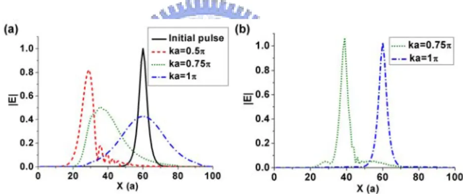
Fig. 10 The hyperbolic-secant (HS) pulse (x0 = 2a) propagates in the CROWs of different wave

vectors at t = 400a/c (a) without Kerr medium and (b) at the soliton propagation criterion by using the 4th _{order Runge-Kutta method. The black solid line in (a) is the incident pulse.}

4.3.2 Soliton propagation in the photonic crystal waveguides

In the PCWs, in order to further evaluate the degree of the pulse broadening arising from high-order dispersions, we define the broadening factor (BF) as σ/σ0, where σ is the

root-mean-square energy of output pulse and σ0 is that of the input pulse. From the BF

of PCWs at different propagating time (T) for ka = 0.6π and 0.75π as shown in Fig. 11 (a), the BF is proportional to 1+T2 as the BF is small, but it is proportional to 1+T when BF

>> 1, which corresponds to the Gaussian pulse propagating in the PCWs [55]. The BF (ka = 0.75π) > BF (0.6π) initially, but becoming reversely with BF (0.6π) > BF (0.75π) after the pulse propagates a span of 60 a/c for x0 = 2a. This is because the BF is mainly

dominated by β3 at the SPC but dominated by β2 after having been severely distorted by

β3. However, when ka = 0.9π and x0 = 2a, the BF would become smaller, which means

that the pulse width becomes narrower and its peak electric field becomes higher. It is due to the opposite signs of β2 and β4 make SPM at γ = γs too strong, especially when β4 is

much larger than β2 and β3 = 0 with small x0. At γ = 0.9γs, the pulse width would

become less broadening and neither further narrowing as time passes as shown in Fig. 11(b). Once the pulse width becomes wider, the high-order dispersions become negligible. The overall self phase modulation at γ = γs should not be apparent.

Fig. 11(a) The broadening factor of ka = 0.6π, 0.75π, and 0.9π and x0 = 2a and 4a of the HS

envelope at the SPC and (b) the broadening factor of γ = 0.9γs and 1γs at ka = 0.9π and x0 = 2a.

The broadening mechanism and the formula to define the SPCs in CROWs and PCWs are similar but the condition (γ or k) to support the SPC is quite different due to the difference of the coupling coefficients. Once when the coupling coefficients are obtained by the PWEM, the pulse broadening and the SPC can be well analyzed by the