RBF-network-based sliding mode control

RBF-Network-Based Sliding Mode Control

Sinn-Cheng L id, Student Member IEEE and Yung-Yaw Chen”, Member IEEE

Department of Electrical Engineering, Lab. 202, National Taiwan University, Taipei, Taiwan, R.O.C.

Electronic Research Laboratory, University of California, Berkeley, CA 94720, USA

1

2

Abstract

-

A sliding mode controller (SMC) design method based on radial basis function network

(RBFN)

is proposed in this paper. Similar to the multilayer perceptron, the RBFN also known to be good universal ap- proximator. In this work, the weights of the RBFN are changed according to some adap- tive algorithms for the purpose of controlling the system state to hit an user-defined sliding surface and then slide along it. The initial weights of the RBFN can be set to small ran- dom numbers, and then on-line tuned auto- matically, no supervised learning procedures are needed. By applying the RBFN-based slid- ing mode controller to control a nonlinear un- stable inverted pendulum system, the simulation results show the expected approx- imation sliding property was occurred, and the dynamic behavior of control system can be determined by the sliding surface.

I. Introduction

Sliding mode control (SMC) strategy has been developed essentially in the literature from the Soviet Union [3][4]. By carefully selecting a suitable sliding suface and applying discon- tinuous control action across the surface, the resulting state trajectory of the control system can be transferred onto the sliding surface and then slide along the surface. There are two phases in the sliding mode control system: 1) hitting phase and 2) sliding phase. In the hit-

ting phase, a hitting control law will be ap- plied to drive the representation point everywhere of state space onto the sliding sur- face. As soon as the representation point hit the surface, the controller turns the sliding phase on, and applies

an

equivalent control law to keep the state on the sliding surface. In ideal situation, when the state trajectory stay on the sliding surface, the control system then has perfect insensitivity respect to the external disturbances as well as the plant parameter variations. Furthermore, even if the system is perturbed such that the representation point is out off the sliding surface, the control system turns on the hitting phase again, and reacts the hitting controller to bring the state toward the sliding surface once more. Therefore, the slid- ing mode control imposes certain constrains on system dynamics. In other words, one can predetermine the sliding surface which domi- nates the dynamic behavior of control system. However, without knowing the mathematical model of system, there is no way to obtain the equivalent control. In the real world, there are many complex industrial processes whose available models can’t be easily developed. Hence, it’s a tough job that designing a model- based sliding mode controller to deal with ill- defined systems. In this paper, we develop a new sliding mode control design strategy based on radial basis jimction network (RBFN) [1][2]. The weights of the RBFN are changed according to some adaptive algorithm for the purpose of controlling the system states 0-7803-2129-4/94 $3.00 0 1994 IEEE

to hit an user-defined sliding surface and then slide along it. The initial weights of the RBFN can be set to small random numbers, and then on-line tuned, no supervised learning proce- dures are needed.

This paper is organized as follows. Sec- tion I1 is a brief description of sliding mode control. In Section 111, an adaptive radial basis function networks is presented for sliding mode controller design. In Section IV, the pro- posed controller is applied to a nonlinear and unstable inverted pendulum system, the simu- lation results verify the efficiency of proposed approach. Conclusions are given in Section V.

11. The Sliding Mode Control

Consider a class of n-th order nonlinear sys- tems, whose dynamics can be represented in the following differential equation

y'"'

=fcv,

y,

...,

y'""')

+

bu, b > 0 (1) wherefl.) is a unknown continuous function, b is a unknown positive constant, and U E R is

the system input and y E R is the system out-

put. To transfer this differential equation to a state space realization, let r be the reference input, and let E = r - y be the error signal. De-

i=1,2,

...,

n, then the system (1) can be repre- sented as the following state equations

A

fine the state e .

-

r(i-1) -y(i-I) = c(i-1) I -

In conventional SMC design, the designer must choose a sliding function. In this paper, we adopt the linear sliding function s = cTe,

where c = [c, c,

...,

c,,] 1IT. While the state reaches the sliding surface s = 0, the equiva-

lent control, U,, , could keep the state stay on

the sliding surface. So, U,, could be derived

from setting the derivative of s, S , equal to

where C = [c1 c2

...

cn-l 0IT. Moreover, in the

sliding mode, s = 0, the system dynamic could be characterized by the following characteris- tic polynomial

D-' + c,-1D-2

+

...

+

c1 = 0

₍₄₎

where

D

A

5.

Therefore, with suitable choice of the coefficients ci , one can obtain a desired equivalent control system.

111. Adaptive Radial Basis Function Networks for Sliding Mode Controller Design Figure 1 shows the block diagrams of RBF network [l], the basis functions we adopted in this paper are all in the form of g(x) = exp[-(T)

1.

Sometime, for the con- venience of notational simplicity, function

s(.)

also expressed as

a m ,

0) in this paper. The

output of the network is

x-m 2

where w = [wl w,

...

wJT, g = [g, g, ... gJT. Without knowing

A.)

and b, there is no way to get ueq, the main purpose here is to use an adaptive RBF network to approximate it. Suppose that the control law has two parts

where U, is obtained from a Rl3F network de-

scribed in the last section. Now, we derived the weights updating law to adjust the weight vector w. Assume there exist a set of weights w' in the universe W, such that (w*)'g

-

U,, is

A

where

Q

= w* - w , and q is a positive con- stant. If we choose the weights updating law as

and the sign of U, is agree with that of sb (this

part will be derived in the next paragraph), then

t.

will has a negative upper bound. Stabilitv consideration: The purpose of the hitting control part, U,

,

in the equation ( 6 ) is

used to draw the state to hit the sliding surface no matter where the initial state is. To achieve such a goal, let's define a Lyapunov function for s

v

- 1 2

s - 2s

the hitting condition which guarantees the sta- bility of sliding mode control system is

ps

=ss <

-qlsI

[7]. Suppose that we know the upper bound offl.) and lower bound of 6, i.e.

Ifl

%f, and 0 < b - I b , then

yields that

ks

I O , and the hitting condition could be satisfied, therefore the system is sta- ble.

Practical consideration: In general, the hitting control part described previously is a high gain bang-bang control. It will generate a very large control force and increase the control cost, which is usually undesired. Therefore, we replace the sign function in (9) by a satura- tion function and modify the control law ( 6 ) by

"

Is'"

, and S is a constant 0, Is1 < S

where

a

=

specified by the designer. Another alternative way to get a better hitting control law by a fuzzy rule base had been developed in our pre- vious work [4].

IV. Simulation Results

In this section, we applied the RBFN-based SMC developed in the last section to control an inverted pendulum system (Figure 2). The dynamics of the inverted pendulum system could be characterized by two state variables:

x,

denotes the angle of the pole with respect to the vertical line, and xz denotes the angular ve- locity of the pole. Neglecting the coefficient of friction, the state equation, which was used for computer simulation, could be expressed as follows

XI

=x2

x 2 =

gsinxl-cosxl ( & x i sinxl-

Af)

; I -

&

C0S*Xl

where g is the gravity constant, 9.8 d s 2 , m, is the mass of the cart, 1.0 kg, m is the mass of the pole, 0.1 kg, 1 is the length of the pole, 1 m

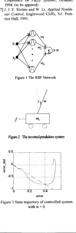
and f i s the input force to the cart. Select c =[2 1IT and q = 100. The activation functions of the single input node and the single output node are all identical. The number of the hid- den nodes is equal to 5 , and their activation functions (the radial basis functions) are se- lected as G,(2, l), G2(0.5, O S ) , G,(O, 0.5), G4(-0.5, O S ) , and G,(-2, l), respectively. The initial weights are all set to zero. By applying the weights updating law (8) and the control law (10) with

a

= 0, i.e. without hitting con- trol, Figure 3 shows the response of the con- trol system. By adding the hitting control part to the system, Figure 4 shows an asymptotical- ly sliding mode can be achieved.

V. Conclusions

In this report, we developed an RE3Fh'-based sliding mode controller, which has the follow- ing characteristics

1 ) Does not require the mathematical model of the system;

2) By applying the hitting control part, the stability of control system can be guaran- teed;

3) Approximation sliding mode was oc- curred;

4) Dynamic behavior of the control system can be specified by an user-defined sliding surface;

5) Does not need any supervise learning pro- cedure. Real time control requirement could be achieved.

Our future research topics focus on hardware implementation of proposed approach and ap- plied to MIMO systems.

Reference

Conference on F u z ~ Systems, Orlando,

1994. (to be appered)

[7] J. J. E. Slotine and W. Li, AppliedNonlin-

ear Control, Englewood Cliffs, NJ: Pren-

tice Hall, 1991.

Figure 1 The RBF Network

[ 1 ] S. Chen, C. F.

N.

Cowan, and P. M. Grant, "Orthogonal Least Squares Learning Algo- rithm for Radial Basis Function Networks,"

IEEE Truns. on Nmrul Networhq vol. 2 ,

no. 2, 1991, pp. 302-309.

[2] J. S. Roger and C. T. Sun, "Functional equivalence between radial basis function networks and fuzzy inference systems",

IEEE Trun. on Nmrul Net., ~01.4, no.1, 1 I

Figwe2 Themvertedpe"sysfem

0.5

I I

w

pp. 156- 159, JAN, 1993.

[3] V. I. Utkin, Sliding modes and their appli- 0

cution in vuriuhle structure .\ystem, Mos-

cow: Mir, 1978 (English translation) [4] U. Itkis, Control bystem of vuriuhle struc-

ture. New York: Wiley, 1976.

[ 5 ] S. C. Lin and C. C. Kung, "A linguistic fuzzy sliding mode controller," Proc. of' [6] S. C. Lin and Y. Y. Chen, "Design of

I \

0.4

0---

error

1992 A.C.C., pp. 1904-1905.

0.5

I I

I I

error

Figure 4 State trajectory of controlled system w i t h a = l