A Study of Exploiting Efficiency of the Duplication-based Algorithm in Distributed Heterogeneous Computing Systems

國立台中教育大學教育測驗統計研究所理學碩士論文

指導教授：賴冠州 博士

A Study of Exploiting Efficiency of the

Duplication-based Algorithm in Distributed

Heterogeneous Computing Systems

研 究 生：劉俊顯 撰

摘 要

近年來，科學應用層面逐漸廣泛，如流體力學、基因分析、氣象預測等等應用比比皆 是。而科學應用需要進行大量的數學或統計運算，如可增進這些常用之數學或統計運算， 則可大量縮短上述科學應用之作業時間。在這些運算中常使用到幾個運算模式，本研究將 針對幾個常見的模式，如:LU, GJE, FFT 加以分析探討。 透過分散式異質性計算系統，可以連結大量的計算資源達到降低各種平行程式之運算 時間。要有效利用計算資源與提昇效率，需要有效的工作排程策略來分配工作所需要的計 算資源與工作的執行次序。工作排程問題是個 NP-complete 的問題，為了降低排程時所需 要的時間，這篇研究提出一個新的直覺式靜態策略複製工作基礎演算法(Dynamic Critical Path Duplication algorithm, DCPD 演算法)，利用工作複製技術有效縮短平行程式執行

時間，以達到有效開發計算資源的目標。 透過實驗結果可以知道，本研究所提出的 DCPD 演算法，效能與開發資源使用率皆優於 其他近年較著名的工作排程演算法(CNPT, HCPFD, TANH)，而且證實這篇文章所提出的演算 法是可以在分散式異質性計算系統達到有效縮短平行程式執行時間與有效開發計算資源的 目標。 關鍵字：分散式異質性系統、有向非循環圖靜態、複製基礎、工作排程、 平行演算法

Abstract

Recently, the scientific applications have been applied in many areas; for example, fluid mechanics, genetic analysis, weather forecast, ..., and so on. Those applications usually need the statistics and the mathematics computation requirements. This study will focus on five common computation patterns (models), including FFT, GJE, LU, fork tree and join tree, as the benchmarks.

This study tries to improve those computation patterns by the Distributed Heterogeneous Computing (DHC) system. The DHC system generally consists of a large number of computing resources. The DHC needs an efficiently scheduling algorithm to schedule tasks to raise performance. But, the scheduling problem is an NP-complete problem. This thesis proposes a novel duplication-based algorithm, which called as the Dynamic Critical Path Duplication (DCPD) algorithm. The DCPD algorithm duplicates tasks to reduce the schedule length and to raise the utilization.

The experimental results show that the performance and the utilization by applying the DCPD algorithm are better than those by applying the other three famous ones: CNPT, HCPFD, and TANH. The experimental results also demonstrate that the DCPD algorithm could reduce the schedule length and exploit utilization effectively in the DHC system.

Keywords ： Distributed heterogeneous computing, directed acyclic graph, duplication-based, task scheduling, parallel algorithm.

Table of Contents

謝詞 ···i 摘要 ···ii Abstract ···iii Chapter 1. Introduction ···5 1.1 Motivations ···5 1.2 Problem Definition ···8 1.3 Objectives ···10 1.4 Restrictions ···15 1.5 Notations ···16

Chapter 2. Related Works ···19

2.1 The TDS Algorithm and The STDS Algorithm ···19

2.2 The TANH Algorithm ···21

2.3 The HNDP Algorithm ···23

2.4 The HCPFD Algorithm ···25

Chapter 3. The Proposed Algorithm ···27

3.1 Definitions ···27

3.2 Node-Processor Selection and Assignment ···30

3.3 Dynamic Critical Path Duplication (DCPD) Algorithm ···31

Chapter 4. Simulation Environment ···37

4.1 Simulation Model ···37

4.2 The Task Graph of Benchmarks ···41

Chapter 5. Experimental Results ···43

5.1 Impact Factors ···43

5.2 Schedule Lengths ···45

5.3 Resource Utilizations ···51

Chapter 6. Conclusions and Future Works ···56

List of Tables

Table 1.1. Terms and their meanings ... 16

Table 3.1. Tasks’ computation costs in different PEs ... 34

Table 3.2. DCPD scheduling steps ... 35

List of Figures

Fig.3.1. An example of unexamined tasks... 28

Fig.3.2. An example DAG... 34

Fig.3.3. Scheduling results for different algorithms. ... 36

Fig.4.1. Simulation environment ... 38

Fig.4.2. Task graphs for different applications. ... 42

Fig.5.1. Average scheduling lengths by varying the number of PEs. ... 46

Fig.5.2. Average scheduling lengths by varying CCRs. ... 48

Fig.5.3. Average scheduling lengths by varying the heterogeneity of PEs. ... 50

Fig.5.4. Average Utilization by varying the number of PEs... 52

Fig.5.5. Average utilization by varying CCRs. ... 53

Chapter 1. Introduction

1.1 Motivations

The statistics and the measurement computations have large computing requirements. Parallel computing could provide the computation capability for these mathematics computation requirements. This research will use five applications as benchmarks in the simulation experiment. Those applications, e.g., FFT, fork, join, Gaussian elimination

and LU-decomposition, usually are applied in the statistics and the measurement.

In both mathematics and statistics, there are may software could be utilized. “Matlab” is a software, which has been widely spread in use. In the last version, the parallel computing module is also supplied. The capability of parallel computing is qualified in order to provide more computation resources to rise computing efficiently.

Due to the advance of the information technology (e.g., CPU, high-speed networks,

etc.), the computational performance increases rapidly. However, there are various scientific applications with computational sensitive requirements; they lead to the related research topics of parallel computing. Therefore, extracting parallelism in scientific applications is an important research issue.

There are many issues of extracting parallelism in parallel applications, such as the software approach (e.g., parallel compiler), and the hardware approach (e.g., pipeline, superscalar, multithread). Recently, many researches focus on distributed computing systems. They utilize existing machines to construct high performance computing

systems. These high performance computing systems may be flexible and extensible. But their extensibility usually makes the high performance system more heterogeneous.

A Distributed Heterogeneous Computing system (DHC) generally consists of a set of different types of geographically distributed suites of computing machines with diverse processing rates, which interconnected by diverse high speed communication links. For applications like weather modeling, fluid flow, image processing, … and so on, distributed heterogeneous computing systems show a great deal of adaptable parallelism and make these applications potential candidates for gaining high performance improvement.

The DHC system would include various hardwires and operating systems. While

their extension capabilities increase, the heterogeneity of the DHC system becomes more

obvious. Beside, DHC systems could offer more commercial and powerful high performance computing environments. The homogeneous computing environments might need dedicated hardware costs. Therefore, the DHC system is more popular and

practical than the homogeneous computing one.

There are at least two distinct features in the distributed heterogeneous computing system: the heterogeneity of the communication network and the heterogeneity of the computational resources. The heterogeneous processor elements are connected by heterogeneous networks in the distributed heterogeneous computing system. The network has the characteristics of the bandwidth limitation and the data transfer latency in the practical distributed heterogeneous computing system. The heterogeneity of

computational resources offers various computing capabilities for the distributed heterogeneous computing system. In the distributed heterogeneous computing system, tasks executed on different processor elements have different execution times. Therefore, effectively exploiting heterogeneous networks and computation resources remains a major challenge in the distributed heterogeneous computing system.

1.2 Problem Definition

In the heterogeneous system, to exploit parallelism is a very important problem. In general, the parallelism within a program may be limited by the efficiency of the system resource. In parallel applications, there are various parallelisms including the fine-grain parallelism and the coarse-grain parallelism. Due to that the performance could be affected by the parallelism exploited in parallel applications, this study focuses on the problem of exploiting the coarse-grain parallelism. This project will consider the utilization of system resources in the distributed heterogeneous computing system.

Because that the distributed heterogeneous computing system has different features, the considerations of exploiting the computing resource in the homogeneous computing systems are different from that in heterogeneous ones. For example, the task scheduled to obtain the earliest starting time in the homogeneous computing system may not be the same task to obtain the earliest complete time in the distributed heterogeneous computing system. Therefore, the resource scheduling problem should be re-considered. It is a very important issue to allocate tasks to processor elements and to arrange their orders to keep the relationship among these tasks. This problem is usually called the task scheduling problem. The scheduling process is to assign the tasks to computing elements (processing elements, PEs) and to order their executions, so that the precedence requirements are satisfied and the minimal completion time is obtained (Braun, Siegel, Beck, Boloni, Maheswaran, Reuther, Robertson, Theys, Yao, Hengsen, & Freund, 1999; Liu, Li, Lai, & Wu, 2006; Li, 2006).

As a rule, there are two categories of task scheduling approaches: the dynamic strategy and the static strategy. In the dynamic scheduling approach, the task assignment and the task scheduling process are dynamically changed. During the task’s execution, the task scheduling algorithm schedules tasks dynamically in the scheduling process. However, in the static scheduling approach, it produces a schedule according the static scheduling algorithm during the compiling time, and the obtained scheduling results could be re-used. Therefore, this study focuses on the static scheduling algorithm strategy.

1.3

Objectives

In the distributed heterogeneous computing environment, an application could be partitioned into a set of tasks, these tasks could be assigned to a set of PEs and arrange their orders to be executed.

The task scheduling problem in the homogeneous computing system is different from that in the heterogeneous computing system. For example, the scheduling algorithms usually distribute even workloads to each computing component in the distributed homogeneous computing system; however, the even-distributed workloads will lead to different completion times in different computing components with various computing capabilities. The computing components with the higher processing capability would wait for the ones with the lower processing capability to finish their tasks’ execution. So the application completing time would be restricted by the computing components with the lower processing capability. This study proposes a novel scheduling algorithm to conform to the system heterogeneity. Therefore, the following issues should be considered:

a. The task which could be issued earlier may not get the earliest completion time. b. There are various parallelisms within the parallel application.

c. It could prompt the utilization of the distributed heterogeneous computing systems to achieve the system’s scalability.

For those reasons, this study will propose a novel algorithm to satisfy the above goals, and to gain the shortest execution time under the suitable system utilization.

In general, a parallel application could be modeled as a directed acyclic graph (DAG). In a DAG, a task is presented as a node, and an edge is presented as the inter-task communication relation and the data dependency between tasks. The weight of a node presents the task processing volume, and the weight of a edge presents the inter-task communication volume between tasks. In this study, we assume that the tasks of a DAG are non-preemptive; in other words, a task executed after other scheduled tasks executed completely on a PE in sequential.

This study proposes a duplication-based scheduling algorithm of the static scheduling algorithm strategy. Applying this algorithm to assign tasks to a system and to schedule these tasks to be executed should consider diverse resource requirements to

gain the minimum completion time(Braun, Siegel, Beck, Boloni, Maheswaran, Reuther,

Robertson, Theys, Yao, Hengsen, & Freund, 1999; Kwok, & Ahmad, 1999). To exploit the heterogeneous computational resource, many researches have focused on solving the NP-complete problem (Ullman, 1975; Garey, & Johnson, 1979) of efficiently scheduling tasks to DHC systems to obtain the near optimal solutions within an acceptable time complexity.

Generally, these static scheduling algorithms could be broadly classified into a variety of categories, such as the list-based algorithm, the clustering-based algorithm and the duplication-based algorithm. The list-based scheduling algorithm (Ranaweera, & Agrawal, 2000; Sih, & Lee, 1993; Park, shirazi, Marquis, & Choo, 1997; Hagras, & Janecek, 2003; Hagras, & Janecek, 2004; Kwok, & Ahmad, 2000) is a classical

scheduling heuristics. The first step of the list-based algorithm, the algorithms sets priorities to all tasks, the priority could be calculated in the static approach or the dynamic approach. By the priorities of the tasks, the algorithm can arrange the schedule order. In the final step, the algorithm allocates the task to the suitable PE repeatedly. The impact of the scheduling is determined by the selection step. So that, the list-based scheduling algorithm is generally an attractive approach in terms of low complexity and

high performance. The main drawback of the list-based algorithm is that each task is

scheduled without sufficient information of subsequent tasks; and hence, the priority assignment does not always lead to the optimal task scheduling.

The clustering-based approach (Gerasoulis, & Yang, 1992; Palis, Liou, & Wei, 1996; Pande, Agrawal, & Mauney, 1994; Pande, Agrawal, & Mauney, 1995) is generally known as a two-phase scheduling approach. The principal idea is trying to reduce the communication cost between inter-tasks to obtain the minimal completion time. For the above purpose, the clustering-based algorithm allocates heavily communicating tasks onto the same PE to reduce the overall communication cost. The clustering-based algorithm includes two phases: the first phase groups tasks into an unbounded number of clusters by clustering heuristics, and then the second phase allocates these clusters onto the PEs by load-balancing heuristics. If the available processors are fewer than the number of the clusters, the algorithm must appropriately merge clusters to fit the number of the available PEs (Ranaweera, & Agrawal, 2000). Although the complexity of clustering-based algorithms is generally lower than that of the list-based ones; the

scheduling performance of clustering-based algorithms is still worse than that of the list-based ones.

The duplication-based approach (Ahmad, & Kwok, 1998; Bajaj, & Agrawal, 2004; Hagras, & Janecek, 2004; Chung, & Ranka, 1992) is another attractive manner for reducing the schedule length. The main idea of this approach is to exploit schedule holes by duplicating the parents of the candidate nodes to more than one PE. The candidate’s starting and finishing time could be reduced by decreasing the communication overhead. The defects of the duplication-based algorithm include the redundant resource consumption and the high complexity. The redundant resource consumption may influence the final makespan. In general, the duplication-based

approaches exhibit their superiority over the list-based and clustering-based ones. The

proposed duplication-based approach is to improve the list-based algorithm to achieve the lower complexity and the higher performance.

There are several approaches to raise the performance in the DHC system, such as improving PEs’ performance, increasing networks bandwidth, and more efficiently exploiting computing resource to advance performance. This study focuses on efficient exploiting computing resources in the DHC environment. It could apply the task duplication approach to reduce the communication overhead between inter-tasks and correcting the priorities dynamically to obtain a more suitable schedule order. As a result, this study extends the classical duplication-based algorithm and it could correct priorities of tasks dynamically in the DHC environment.

The remainder of this thesis is organized as follows. Chapter 2 introduces the newly static duplication-based heuristics. Chapter 3 presents the proposed algorithm. Chapter 4 describes the simulation environment. Experimental results and performance analyses are provided in Chapter 5. Concluding remarks and future works are then offered in Chapter 6.

1.4 Restrictions

This research proposes a duplication-based algorithm in the distributed heterogeneous computing environment. Later, the restrictions about this research are listed.

z The bounded number of heterogeneous processor elements is known. z The number of tasks within an application could be known.

z The PE’s information could be known in advance. z The network bandwidth could be known previously.

z The computation volumes of all tasks are known beforehand. z The communication volumes of inter-tasks are known formerly.

1.5 Notations

The related terms and the meanings used in this thesis are given in Table 1.1. Below is the table of contents, indicates some symbols are used in this research.

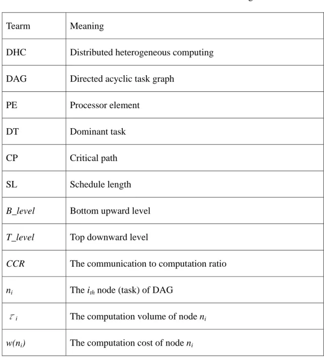
Table 1.1. Terms and their meanings

Tearm Meaning

DHC Distributed heterogeneous computing

DAG Directed acyclic task graph

PE Processor element

DT Dominant task

CP Critical path

SL Schedule length

B_level Bottom upward level

T_level Top downward level

CCR The communication to computation ratio

ni The ith node (task) of DAG

τ

i The computation volume of node ni

Ci,j

The communication volume of directed edge form the ni to the

node nj

ei,j

The communication cost of directed edge form the ni to the node

nj

pi The ith processor element

α

i The execution rate of processor element p_i

β

i The communication rate from processor element pi to processor

element pj

qi,j

The communication channel from processor element pi to

processor element pj

est(ni) The earliest starting time of node ni

ect(ni) The earliest completion time of node ni

lct(ni) The latest completion time of node ni

ST(ni,j) The starting time of node ni on processor element pj

FT The finish time

EST The earliest starting time

EFT The earliest finish time

LST The latest must starting time

AEST(ni,j)

The absolute earliest starting time of node ni on processor

element pj

ALST(ni,j)

The absolute latest starting time of node ni on processor element

pj

pred(ni) The set of immediate predecessor nodes of node ni

fpred(ni) The favorite predecessor nodes of node ni

fproc(ni)

The favorite processor of task ni, assigning task ni to the

processor will yield a minimum completion time for task ni

SL The Schedule length of the DAG

RT(pi) The time of pi is available

DAT(ni, pi) The data arrival time of the ni on pi

Chapter 2. Related Works

In this chapter, four well-known duplication-based scheduling algorithms are described, including the Task Duplication-based Scheduling (TDS) algorithm, the Scalable Task Duplication-based Scheduling (STDS) algorithm, the Task Duplication-based Scheduling Algorithm for Network of Heterogeneous Systems (TANH) algorithm, the Heterogeneous N-Predecessor Duplication (HNDP) algorithm and the Heterogeneous Critical Parents with Fast Duplicator (HCPFD) algorithm. These algorithms are discussed in the following sections respectively.

2.1 The TDS Algorithm and The STDS Algorithm

The TDS algorithm (Ranaweera, & Agrawal, 2000) is a duplication-based scheduling algorithm. It includes three steps: the first step is to calculate est,ect, fpred,

fproc1 to fprocn and level for each task from the DAG’s entry node to the exit node in a

top-down fashion. The level value is the highest value of the sum of the computation cost from the node to the exit node along different paths. The queue is built by all the tasks in ascending order by the levels. The second step is to calculate lact and last for each task in a bottom-up fashion. The third step is to cluster tasks to generate an initial set of clusters using the less number of processors. The algorithm performs the following steps repeatedly. The first step is to find the first un-examined task in the

task’s fproc order to cluster tasks. If the fpred is un-examined or it is on the critical path, the algorithm clusters the fpred of the task. If there is more than one predecessor, the algorithm selects the predecessor with the lowest computing cost on the processor. The final step is to exploit the task duplication to avoid communications. If the predecessor of the task is not the favorite one, the previous tasks are replaced by the favorite tasks by the order of the lengths of the paths in clusters. The replaced tasks are scheduled on a new processor. The TDS algorithm uses a task duplication approach if the favorite predecessor is not in the same cluster. But, replacing all tasks which are scheduled prior to its favorite task in the new cluster might increase the inter-processor communication overhead.

The STDS algorithm (Ranaweera, & Agrawal, 2000) is similar to the TDS one; it performs task duplication is the same as the TDS algorithm. However, the STDS algorithm improves the requirement that the number of processors is larger than that of the available processors. It merges clusters to match the actual number of processors.

Although the STDS algorithm works well in the unbounded number of processors environment. But, in general, the number of processors is bounded; the merging approach could be improved to obtain a better performance.

2.2 The TANH Algorithm

The TANH algorithm (Bajaj, & Agrawal, 2004) is a cluster-based and duplication-based combined algorithm. It is extended from the STDS algorithm (Ranaweera, & Agrawal, 2000) and is modified to get the optimal solution for the DAGs.

The TANH algorithm starts at calculating each node’s est, ect, favorite processors and level values. It obtains est and ect by using the mean computation costs of all PEs. The TANH algorithm determines favorite processors from fp1 to fpn by sorting the completion time of the nodes over all processors by ascending order under the assumption that there are n processor elements. In other words, the fp1 of the node indicates the node which can obtain the minimal completion time on the processor element. The ect and est values of the node are calculated on the favorite processor. The

level value of the node is the longest path along different paths from the node to exit node.

The level value would be obtained by finding the node’s computation cost, and it excludes communication costs between inter-nodes.

The TANH algorithm finds the exit node’s ect value, the exit node’s lact sets to be

ect. Calculating the lact and last values for each node is by the bottom-up fashion. The lact is the latest allowable completion time of the node and the last is the latest allowable

start time of the node. The fpred is the favorite predecessor which is defined as the predecessor with the largest value of the sum of the earliest completion times and the communication costs among all the predecessors. The TANH algorithm sets the entry

node’s fpred value to be null. The above procedure completes after building the table of those variables.

In the second step, the TANH algorithm generates initial clusters by pushing tasks into the queue by the level values of all nodes in an ascending order. By clustering tasks, each clustering procedure chooses the first unexamined node in the queue. After clustering phase is finished, it assigns the top task in the cluster to the first available favorite processor. Then, if each task’s predecessor is not the critical node or it has been assigned, the algorithm assigns the predecessor to the current cluster, and that predecessor is set to be examined recursively until reaching the entry node; if the fpred had been selected, the algorithm selects the unexamined predecessor in the queue and sets to be examined.

In the third step, if the number of available processors is less than the number of required processors, the TANH algorithm performs the processor reduction procedure to merge clusters to reduce the number of clusters into the number of available processors.

The disadvantage of the TANH algorithm is that the number of required processors is more than the number of available processors generally; otherwise, the performance would be degraded. Therefore, the algorithm performs the processor reduction procedure to merge two clusters by the largest and the least values of summing the computation costs of tasks in the processor. The above procedures lead to the performance downward seriously.

2.3 The HNDP Algorithm

The HNDP algorithm (Baskiyar, & Dickinson, 2005) is extended from the Decisive Path Scheduling (DPS) algorithm (Park, shirazi, Marquis, & Choo, 1997). The DPS algorithm has shown the efficient for homogeneous environment. The HNDP algorithm improves the DPS algorithm to suit the heterogeneous environment, and it extends the assign phase from the list-based algorithm to the duplication-based algorithm.

The DPS algorithm starts at transforming an input DAG to a new DAG which has only one entry node and only one exit node. The transform can be done by adding a pseudo entry node and a pseudo exit node, such that their computation cost are zero. So DPS algorithm can identify the decisive paths to all the nodes of the new DAG.

The DPS algorithm first calculates the top and bottom distance for each node using the mean computation cost. The top distance is the longest distance between the entry node and the node excluding computation cost of the node, and the bottom distance is the longest distance between the node and the exit node include computation cost of the node. The length of each node’s decisive path (DP) is the sum of the top distance and the bottom distance.

After building the DP for each node, the DPS algorithm will create a task_queue, whose sequence is the order to schedule the DAG. The DPS algorithm creates the task_queue starting with the DAG’s entry node and traversing the critical path (CP) to the exit node. In fact, the CP is a set of the nodes which have the largest DP from an entry

node. The critical path node (CPN) is the node on the CP. After all of the node’s predecessors have been added to the task_queue, the node can be added to the task_queue. If the node has at least one predecessor which isn’t in the task_queue, DPS attempts to schedule all of the node’s predecessors into the task_queue in a top-down fashion.

In the assign phase, The HNPD algorithm is an insertion-based algorithm. It uses the insertion policy to find the slot time in processors. The HNPD algorithm selects PEs according by calculating the node’s earliest complete time of all nodes. Once the node has been assigned to the processor, the HNPD algorithm attempts to duplicate predecessors of the node to reduce the actual complete time of the task. The algorithm duplicates the node’s predecessor, if there is the slot time which is large enough to duplicate the favorite predecessor between the recently assigned task and the preceding task on the selected PE. The duplication procedure is performed repeatedly for each predecessor in the order from the most favorite task to the least task. After HNPD duplicating each predecessor of the node, to duplicate the duplicated tasks’ predecessors recursively until no further duplication is possible.

The advantage of the HNPD algorithm is that the duplication procedure and the assignment procedure use the insertion fashion. The HNPD algorithm’s duplication procedure can duplicate tasks as possibly to reduce the execution time of the DAG. The HNPD algorithm also doesn’t to consider that the critical path might be changed during assign tasks and duplication tasks to processors. The HNPD algorithm can’t obtain more information during the determined schedule order.

2.4 The HCPFD Algorithm

THE HCPFD algorithm (Hagras, & Janecek, 2004) is based on the CNPT list-based algorithm (Hagras, & Janecek, 2003) and it extends the CNPT algorithm. The HCPFD algorithm improves the assign phase of the CNPT algorithm which modify assignment phase from the list-based algorithm to the duplication-based algorithm.

There are two phases of the CNPT algorithm. In the first phase, the CNPT algorithm determines the schedule order of all tasks. In the second phase, the CNPT algorithm depends on the schedule order in the first phase to assign a task onto the PE with the minimal complete time.

In the listing phase, the CNPT algorithm separates all task of a DAG into a set of parent-trees. All the root-nodes of parent-trees are the nodes on the critical path which called the critical node (CN). The CNPT algorithm applies a empty queue and an auxiliary stack during scheduling. The algorithm starts at pushing CNs into a auxiliary stack by their ALSTs. If the top node of a stack has more one unscheduled parents, those parent nodes are pushed into the stack. Otherwise, the top node of a stack is popped, and it is queued into the queue of schedule order.

In the assign phase, the CNPT algorithm depends on the schedule order of the listing phase, to assign task onto PE which has the minimal complete time.

The HCPFD algorithm extends the CNPT algorithm in the assign phase for reducing the makespan. At each assign step, the HCPFD algorithm assigns the candidate task to a PE which has the minimal complete time, and then duplicates its critical parent node on

the time slot between the candidate task and the previous task on the same PE, if this slot time is enough. This duplication procedure can raise the candidate task’ complete time on the PE.

The HCPFD algorithm reduces the makespan effectively by the duplicating critical parent nodes approach. But it just bases on the list scheduling and make task duplication simply, it doesn’t neither consider that critical path which could change during assign phase nor check the slot time between the data arrival time of the duplication task and candidate one.

Chapter 3. The Proposed Algorithm

3.1 Definitions

The classical scheduling algorithms adopt the macro-dataflow model (Banal, Kumar, & Singh, 2003) to be the program model. This program model assumes that the communication is contention-free (Bajaj, & Agrawal, 2004). In this study, a program is presented as a directed acyclic graph (DAG) ( Liu, Li, Lai, & Wu, 2006; Li, 2006). The DAG is defined as G = (N, E, T, C), where N is the set of task nodes, T is the set of node computation volumes, E is the set of communication edges that define a partial order or

precedence constraints on N, and C is the set of communication volumes. The value

τ

I

∈T is the computation volume for ni ∈ N. The value of can ∈ C is the communication

volume occurring along the edge eij ∈ E, where ni, nj ∈ N.

In this model, a task is assumed to be non-preemptive, and a PE is assumed to execute one task at a time (i.e., no multitasking). Precedence constraints occur only when one task’s execution is deferred by waiting for data receiving; and, resource contentions arise when the resource is occupied by some other tasks. After that precedence constraint is satisfied and that resource contention is removed, the task’s execution would be triggered.

the scheduling process, a task is called examined after it is scheduled to some PE and

unexamined before it is scheduled to some PE (Liu, Li, Lai, & Wu, 2006; Li,2006). The

set of the unexamined tasks consists of the ready set, the partially ready set and the unready set. In the ready set, the task’s immediate predecessors are all examined. In the partially ready set, at least one of the task’s immediate predecessors is examined and at least one of its immediate predecessors is unexamined. In the unready set, none of the task’s immediate predecessors of any unready task is examined. Fig.3.1 shows these

situations. After task na is scheduled to some PE, it is examined. The unexamined set

includes {nb, nc, nd, ne}, in which the set {nb, nc} is the ready set, the set {nd} is the

partially ready set, and the set {ne} is the unready set. Here, we define the u-level(ni) of

an unexamined ready node ni as the shortest average length from entry nodes to it.

a b _c d examined unexamined e

Fig.3.1. An example of unexamined tasks.

Generally, most of the proposed algorithms fail to consider the problem of exploiting schedule holes (Lai, Fang, Sung, & Pean, 2003; Baskiyar, & Dickinson, 2005). The DCPD algorithm employs these schedule holes by inserting the duplicated parent

tasks of a candidate task for advancing the earliest starting time of this candidate task. On the one hand, the utilization of the PE could be raised, and on the other hand, the earliest starting time of some task could be advanced to bring the shortening of the final generated schedule length.

3.2 Node-Processor Selection and Assignment

A dominant task must be identified at each scheduling step, and the challenge is to find the selection priority that could well reflect the critical nodes in the context of scheduling. To identify the dominant task in the DCPD algorithm, all the ready tasks are considered, and the task ndt with the maximal value of b-level(ndt) - u-level(ndt) +

)) ( ( dt

dt α p n

τ × is identified as the dominant task (DT). The priority function is derived

from three conditions, (a) the task that could be issued earlier should be scheduled first, (b) the one having the larger computation cost should also be scheduled first, and (c) the task that could be scheduled to the PE with the larger remainder should be scheduled first.

Therefore, we mix these conditions to obtain the priority function.

For a node, a PE that allows one node’s earliest start time is not necessarily the same

PE that allows the node’s earliest finish time in the heterogeneous environment.

Therefore, the candidate node, ndt, is scheduled to the PE that allows this node’s earliest

completion time to be obtained. In this study, the dominant predecessor (DP) is the predecessor of a task which belongs to the partial ready set or the unready set; when the DP finishes executing, the task’s execution would be triggered by satisfying precedence constraints and removing resource contentions. In another words, the advance of the earliest starting time of a task would be restricted by the task’s dominant predecessor.

3.3 Dynamic Critical Path Duplication (DCPD) Algorithm

The DCPD algorithm is presented below. First, the DCPD algorithm initializes variables and finds the average execution rates and the average communication rates for all heterogeneous PEs. The DCPD algorithm initially assumes that each task is assigned to one virtual PE and that the communication overhead between tasks is assumed to be the average communication rate times the communication volume between tasks. Then the DCPD algorithm estimates b-levels for all tasks by using the average execution rates for all heterogeneous PEs bottom-up. Let the tasks without predecessors be in the ready set. When the ready set is not empty, the DCPD algorithm repeats the following steps:

1. Calculate the priorities of tasks in the unexamined ready set. The priority function, priority(ni), of a task ni is τ_i×α(p(n_i)) + b-level(ni) - u-level(ni).

2. Let the dominant task, ndt, be the task with the maximal priority in the ready set.

3. Find out the PE, p(ndt), where the ect(ndt) could be obtained by insertion policy.

4. Find out the dominant predecessors, ndp, and the related data ready time, drt(ndp).

5. If there is an enough free time slot from drt(ndp) to est(ndt) to schedule ndp to p(ndt),

then schedule the duplicated ndp to p(ndt) to advance the est(ndt) by the insertion

policy.

6. Allocate ndt to p(ndt), and make ndt examined.

7. Re-check the ready set, and re-compute the u-levels for all tasks in the unexamined ready set.

8. Repeat steps 1 to 7 until all tasks are examined.

In the DCPD algorithm, the time complexity for calculating the b-level is O(|N|+|E|).

The while loop is executed in O(|N|), finding ndt and its related PE is O((|N|+|E|)|P|).

Finding out the ndp needs O(|N|) steps. Therefore, the time complexity of the DCPD

algorithm is O((|N|+|E|)|N||P|). Consequently, in practical applications, the complexity of the DCPD algorithm is reasonable.

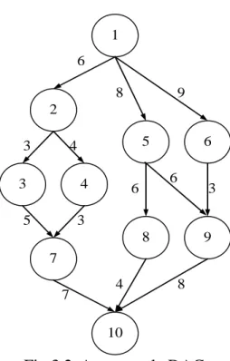
3.4 A simple Example

In the following, we introduce an example to show the superiority of the DCPD algorithm. In order to simplify the analyzing process, we assume that the computation cost (i.e., τi×α(p(ni))) of all tasks in all PEs are estimated in the Table 3.1 (e.g., the

computation costs of task n1 are 5, 3, 4 in PE1, PE2, and PE3 respectively), and that the

communication rates of all communication channels are all one, therefore the numbers listed along edges are communication volume and also could be considered as the communication costs when the parent node and its child node are scheduled in different

PEs (for example, when tasks n1 and n2 are scheduled in different PEs, the

communication cost between tasks n1 and n2 are 6).

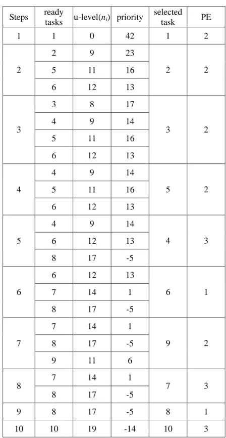
Next, we could calculate the average computation costs and b-levels for all tasks. When the set of unexamined tasks is not empty, the DCPD algorithm selects one candidate task, ndt, to be scheduled to its corresponding PE. Tasks with no predecessors

are selected first. The whole process steps are listed in Table 3.2. The scheduling results obtained from the TANH, HCPFD and DCPD algorithms are shown in Fig.3.3.

9 8 8 4 7 3 6 6 3 5 4 3 6 2 6 5 3 4 10 7 8 9 1

Fig.3.2. An example DAG.

Table 3.1. Tasks’ computation costs in different PEs PEs

Task ni

PE1 PE2 PE3

1 5 3 4 2 3 2 7 3 3 4 8 4 7 5 3 5 5 2 5 6 3 4 8 7 4 2 3 8 2 3 4 9 4 5 3 10 6 4 5

Table 3.2. DCPD scheduling steps

Steps ready

tasks u-level(ni) priority

selected task PE 1 1 0 42 1 2 2 9 23 5 11 16 2 6 12 13 2 2 3 8 17 4 9 14 5 11 16 3 6 12 13 3 2 4 9 14 5 11 16 4 6 12 13 5 2 4 9 14 6 12 13 5 8 17 -5 4 3 6 12 13 7 14 1 6 8 17 -5 6 1 7 14 1 8 17 -5 7 9 11 6 9 2 7 14 1 8 8 17 -5 7 3 9 8 17 -5 8 1 10 10 19 -14 10 3

(a) TANH 0 5 10 15 20 25 30

PE1 PE2 PE3

4 1 2 3 7 4 9 8 10 1 5 6 (b) HCPFD (c) DCPD 0 5 10 15 20 25 30

PE1 PE2 PE3

4 1 2 3 7 9 8 10 1 5 6 40 35 40 35 2 1 0 5 10 15 20 25 30

PE1 PE2 PE3

1 2 3 5 8 7 1 6 4 9 10 40 35 7 5 : Duplicated task

Chapter 4. Simulation Environment

In this chapter, the simulation environment would be discussed in the following sections respectively. Section 4.1 introduces five common benchmarks used in the simulation environment. Section 4.2 introduces the simulation environment and the related works.

4.1 Simulation Model

This study runs the experiments in a simulation environment, which consists of three modules: the task graph generator module, the parameter generator module and the simulation program module. First module produces the DAG generated by the program structure of the application. Second, the parameter generator module defines the heterogeneity of the simulation environment. After receiving information of the simulation environment from the above two modules, the simulation programs (algorithms) can be executed in the simulation program module. Third, the data is obtained by the simulation programs. The simulation environment is illustrated in Fig.4.1.

Parameter

Generator

Module

Task Graph

Generator

Module

Simulation

Program

Module

Experiment

Results

Fig.4.1. Simulation environment

The task graph generator module generates the volumes of the computation and the communication in the task graphs. The processing step of the task graph generator module would be discussed more detailed in section 4.2.

The communication to the computation ratio (CCR) is the ratio of the average communication rate to the average computation rate. If the CCR value of the application’s task graph is greater than one, which can be called as communication-sensitive. When the application is high communication-sensitive, its

CCR value is very high. In contrast, the application is called as computation-sensitive,

if its CCR value of the application’s task graph is less than one. In this study, the value of the CCR value is set to be 0.1, 0.3, 0.5, 0.7, 0.9, 1.0, 2.0, 4.0, 6.0, 8.0 or 10.0.

In this study, the simulation environment adopts the consistent heterogeneity (i.e., when any task that runs on a PE faster than another PE implies that the execution time of

parameter generator module generates the system parameters of the simulation environment such as computation and communication rates. As mentioned, a DHC system is represented as M = (P, Q, A, B) (Liu, Li, Lai, & Wu, 2006; Li,2006), where

P={pi|pi∈P, i=1,..,|P|} is the set of heterogeneous processing elements (PEs), A =

{

α

(pi)|

α

(pi)∈A, i=1,..,|P|} is the set of the execution rates for heterogeneous PEs,

α

(pi) is

the execution rate for pi, Q = {q(pi,pj)|q(pi,pj)∈Q, i, j= 1..|P|} is the set of communication

channels, q(pi,pj) is the communication channel from pi to pj, and B = {

β

(pi,pj)|

β

(pi,pj)

∈B, i, j=1..|P|} is the set of the transferring rates for communication channels from pi to

pj. Each PE has a coprocessor to deal with communications, which allow computations

and communications that are independent of each other to be overlapped. Let

τ

i×

α

(pj)

be the computation cost when task ni is allocated to pj, and cij×

β

(pk,pl) be the

communication cost from task ni to task nj, where ni is allocated to pk and task nj is

allocated to pl.

The parameters of system heterogeneity are

α

(pj) and

β

(pk,pl), which adjust the

range of the heterogeneity of the simulation environment.

α

(pj) and

β

(pk,pl) are

generated by the normal distribution, with increasing the various value of

α

(pj), the

computation heterogeneities of the simulation system would be raised. On the other hand, with increasing the various value of

β

(pk,pl), the communication heterogeneities of

the simulation system would be raised. As the number of variances increasing, the system heterogeneities become more obvious. It has been known that the system

heterogeneity may affect the quality of the schedule produced by heuristics. In order to

compare the result between the execution rate and the transfer rate, the number ofPEs are

set to 2, 4, 8, 16, or 32. The variance of the execution rates,

α

(pi), of the heterogeneous

PEs is defined as the heterogeneity of computational power. Assumption the distribution of the execution rate is normally distributed: its mean value is 10, and the variance may be set to 0.2, 0.4, 0.6, 0.8, 1.0, 2.0, 4.0, 6.0, 8.0 or 10.0. However, the variance of the transfer rates,

β

(pi,pj), for communication channels is defined as the

heterogeneity of communication mechanisms. The solution of the distribution of the transfer rate is also normally distributed: its mean value is 10, and the variance may be set to 0.2, 0.4, 0.6, 0.8, 1.0, 2.0, 4.0, 6.0, 8.0 or 10.0.

The simulation program module performs the algorithms by using the parameters generated by parameter generator module, and then generates the makespans. All the simulation programs are coded by C language, include the parameter generator and all the schedule algorithms. The simulation environment is built on the Linux operating system which version is Fedora Core 4, and the compiler is g++. The system is installed on the IBM Xserver 206, its specification include Intel Pentium IV 3.0G HZ CPU with Hyper-Thread, 1G DDRII RAM and two SCSI 36G harddisks. There are four algorithms performed and compared. They are the CNPT algorithm, the HCPFD algorithm, the TANH algorithm and the DCPD algorithm. After obtaining the schedule lengths from the simulation environment that would be analyze the output data from the simulation module and conclude the experimental results.

4.2 The Task Graph of Benchmarks

The applications can be partitioned into several sub_tasks, each sub_task is a program segment which couldn’t be divided. Those segments could be presented as the nodes in the DAG. The beginning segment presents the entry node, and the exit node as the last segment. The precedence relation between two sub_tasks can be presented by a direct line.

This study proposes five common applications as benchmarks for experiments evaluation in the simulation environment. The five benchmarks includes the Fast Fourier Transformation (FFT) (Chung, Liu, & Liu, 1995), the fork task graph, Gaussian elimination algorithm (Wu & Gajski, 1990), the join task graph, and LU-decomposition algorithm (Lord, Kowalik, & Kumar, 1983). Fig.4.2 indicates the five practical applications’ miniature examples.

The computation weight of each node and the communication weight of each edge are given by their in-degree and out-degree relations. The benchmark generator generates the volumes’ value for each task node of the application’s DAG. The volumes of computation and communication required for each task node are pre-determined according to the program structures of the applications.

(a) a Gaussian elimination task graph n14 n13 n1 n2 n3 n4 n5 n6 n7 n8 n9 n10 n12 n11

(b) a LU-decomposition task graph

n1 n2 n3 n4 n5 n6 n7 n8 n9 (c) a FFT task graph n1 n14 n2 n3 n4 n5 n6 n7 n8 n9 n10 n11 n12 n13 n15 n1 n2 n3 n4 n5 n6 n7 n8 n9 n10 n11 n12 n13

(d) a fork task graph

(e) a join task graph

n1 n2 n3 n4 n5 n6 n7 n8 n9

n10 n11 n12

n13

Chapter 5. Experimental Results

In this chapter, four proposed algorithms are evaluated. They are the CNPT algorithm, the HCPFD algorithm, the TANH algorithm, and the DCPD algorithm. To demonstrate the feasibility of the DCPD algorithm, the experimental results by evaluating five practical applications are presented in this section. The five practical applications includes the Gauss–Jordan Elimination, the Fast Fourier Transformation, the LU factoring, the Fork trees and the Join trees, whose graphic sizes vary from a minimal of 378 nodes to a maximum of 511 nodes. The computation/communication volumes required for each task node are pre-determined according to the program structures for the different applications.

The comparisons are based on the schedule lengths and the utilizations, which are generated by these algorithms. In section 5.1, the impact factors and the statistic analysis are discussed. In section 5.2, the comparisons of schedule lengths are illustrated. In section 5.3, the comparisons of processor elements’ utilizations are presented.

5.1 Impact Factors

The granularity of the application would affect scheduling result. In general, the granularity could classify fine-grain and coarse-grain. If the CCR is greater than one, the application’s granularity is called fine-grain. In other words, if a application’s

granularity is called coarse-grain, the CCR is less than one. The performance generated by different CCRs has been discussed.

If the application’s granularity is fine-grain, the communication cost is lower than

the computation cost. This situation would cause the little schedule hole. The

insertion policy would exploit those schedule holes to perform tasks earlier.

In other words, if the application’s granularity is coarse-grain, the communication cost is higher than the computation cost. In this circumstance, it would cause a large time slot on the PEs. The DCPD algorithm exercises duplicating tasks to reduce schedule length and to increase utilization of PEs.

The DCPD algorithm considers the critical path could change during scheduling by assigning tasks on PEs. The DCPD algorithm uses the priority values to select the dominant tasks, and these priorities would be computed dynamically. The selection of dominant tasks could be more exactly by the dynamically priority, which could reduce the schedule lengths efficiently.

5.2 Schedule Lengths

In general, the HCPFD algorithm outperforms the CNPT and the TANH ones; therefore, only the key issues between the HCPFD and the DCPD algorithms are presented in the follows. First, the HCPFD algorithm does not consider the effect that the critical path may dynamically change in the scheduling process due to that the

scheduling sequence is determined in the listing phase. Second, the HCPFD algorithm

tries to duplicate the candidate’s critical parent at the idle time slot between the starting time of the candidate’s critical parent and the last previous task assigned in the same PE. However, the DCPD algorithm duplicate the candidate’s critical parent at the idle time slot from the data ready time of the candidate’s critical parent to the starting time of the candidate node. Third, the DCPD algorithm initially assigns each task to one virtual PE, and avoids from re-evaluating the ready-task-PE pairs in every scheduling steps.

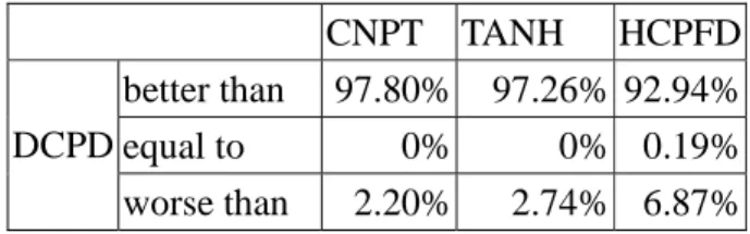
Table 5.1. Algorithm Comparison in terms of Scheduling Lengths

CNPT TANH HCPFD better than 97.80% 97.26% 92.94% equal to 0% 0% 0.19% DCPD

worse than 2.20% 2.74% 6.87%

Comparatively, the DCPD algorithm outperforms the CNPT algorithm, the TANH algorithm and the HCPFD algorithm in terms of the schedule lengths, as shown in Table 5.1. The average schedule lengths obtained by the DCPD algorithm are shorter than

those obtained by the HCPFD algorithm in 92.94% cases, by the TANH algorithm in 97.26%, and by the CNPT algorithm in 97.80% cases. In general, DCPD algorithm outperforms the CNPT, the TANH and the HCPFD in terms of the schedule lengths, by handling the heterogeneity of computational power and that of communication mechanisms. (a) FFT 40000 80000 120000 160000 200000 2 4 8 16 32 PE # S ch edu le L en gt h CNPT HCPFD TANH DCPD (b) Fork 0 50000 100000 150000 200000 250000 300000 350000 400000 450000 2 4 8 16 32 PE # S chedu le L en g th CNPT HCPFD TANH DCPD (c) GJE 0 100000 200000 300000 400000 500000 600000 2 4 8 16 32 PE # Sc hedu le L ength CNPT HCPFD TANH DCPD (d) Join 0 50000 100000 150000 200000 250000 300000 350000 2 4 8 16 32 PE # S che du le L en gt h CNPT HCPFD TANH DCPD (e) LU 400000 600000 800000 1000000 1200000 1400000 2 4 8 16 32 PE # Schedule L ength CNPT HCPFD TANH DCPD

Fig.5.1 shows the average scheduling lengths for different applications are given by varying the number of PEs. Generally, the schedule length which generated by the DCPD algorithm decreases gradually as the number of PEs increases. In Fig.5.1 (a) ~ (e), showing the average schedule lengths are generated by the DCPD algorithm are shorter than that generated by other three algorithms. It shows the DCPD algorithm outperforms others. The main reason is that the DCPD algorithm could capture the track of the dominant nodes in each scheduling step.

In Fig.5.1 (c), the schedule lengths obtained by the DCPD algorithm are obvious shorter than those obtained by other three algorithms when the number of PEs are smaller than 16. The main reason is that the scope of the application’s parallelism is limited (only 378 ~ 511 nodes) to simplify the experimental process. The same situations are also shown in Fig.5.1 (a) ~ (e).

In Fig.5.1 (c) ~ (d), the performance of the GJE and the JOIN applications generated by the TANH algorithm is similar to that of the other algorithms. The main reason is that both the GJE and the JOIN applications have many join structures.

(a) FFT 50000 70000 90000 110000 130000 150000 170000 190000 210000 230000 0.1 0.3 0.5 0.7 0.9 1 2 4 6 8 10 CCR Sc hedule L eng th CNPT HCPFD TANH DCPD (b) FORK 70000 90000 110000 130000 150000 170000 190000 210000 0.1 0.3 0.5 0.7 0.9 1 2 4 6 8 10 CCR Sche dule L engt h CNPT HCPFD TANH DCPD (c) GJE 120000 140000 160000 180000 200000 220000 0.1 0.3 0.5 0.7 0.9 1 2 4 6 8 10 CCR Schedul e L engt h CNPT HCPFD TANH DCPD (d) JOIN 80000 100000 120000 140000 160000 180000 200000 220000 240000 0.1 0.3 0.5 0.7 0.9 1 2 4 6 8 10 CCR Sc he du le L ength _CNPT HCPFD TANH DCPD (e) LU 0 500000 1000000 1500000 2000000 2500000 0.1 0.3 0.5 0.7 0.9 1 2 4 6 8 10 CCR Sc he du le L en gt h CNPT HCPFD TANH DCPD

Fig.5.2. Average scheduling lengths by varying CCRs.

Fig.5.2 (a) ~ (e) shows that the average scheduling lengths increase as the communication to computation cost ratio (CCR) increases. The main reason is that, when CCR is greater than one, the communication cost has a greater effect upon the scheduling lengths obtained in the scheduling process. Due to that the

DHC system allows computations and communications which are independent of each other to be overlapped, the scheduling length would be dominated by scheduling communications among tasks when CCR is smaller than one.

In Fig.5.2 (a) and Fig.5.2 (b) show the scheduling lengths of the CNPT algorithm and the HCPFD algorithm a bit of decreasing when the CCR equals to one. The reason is that the CNPT algorithm is fix the critical path, the critical node would assign to the same PE, the system parallelism could not be exploited. For the FORK application and the GJE application, their DAG has more fork task procedure, the reason leads the similar variation in these two applications. After

CCR is greater than one, the performance result is the same as previous

discussions.

Fig.5.3 (a) ~ (e) shows the average scheduling lengths for different applications by varying the heterogeneity of PEs. In general, the variation of schedule lengths varies very rapidly. However, in Fig.5.3 (a) ~ (e), showing the average schedule lengths are generated by the DCPD algorithm are shorter than that generated by other three algorithms. It shows that the DCPD algorithm outperforms others. The main reason is that the DCPD algorithm could exploit the insertion policy to execute task earlier to raise performance.

(a) FFT 50000 70000 90000 110000 130000 150000 170000 190000 0.2 0.4 0.6 0.8 1 2 4 6 8 10 PE Various Schedul e L engt h CNPT HCPFD TANH DCPD (b) FORK 50000 100000 150000 200000 250000 300000 0.2 0.4 0.6 0.8 1 2 4 6 8 10 PE Various Sc he du le L ength CNPT HCPFD TANH DCPD (c) GJE 100000 120000 140000 160000 180000 200000 220000 240000 0.2 0.4 0.6 0.8 1 2 4 6 8 10 PE Various Sc hedule L engt h CNPT HCPFD TANH DCPD (d) JOIN 60000 80000 100000 120000 140000 160000 180000 0.2 0.4 0.6 0.8 1 2 4 6 8 10 PE Various Sc he du le L en gt h CNPT HCPFD TANH DCPD (e) LU 400000 500000 600000 700000 800000 900000 1000000 1100000 0.2 0.4 0.6 0.8 1 2 4 6 8 10 PE Various Schedul e L en gt h CNPT HCPFD TANH DCPD

5.3 Resource Utilizations

The Resource utilizations are the utilization of the PEs’ computation resource. In this paper, the utilization is defined as below:

Utilization= AET / (schedule length × PE #) ,

where AET is defined all tasks execute time on all PEs include over all duplication tasks.

Fig.5.4 (a) ~ (e) shows that the average system utilization obtained by the CNPT, TANH, HCPFD and DCPD algorithms decreases gradually as the number of PEs increases. It implies that the system utilization reduces as the number of PEs increases. The utilization of the TANH algorithm is higher than others, but the schedule length of the TANH algorithm is not shorter than others, it indicates the TANH algorithm has redundant duplication, those duplication tasks could addition the schedule length.

In Fig.5.4 (c), when the number of PEs is equal to 32, the utilization of the DCPD algorithm is less than that of the HCPFD algorithm and that of the TANH algorithm. The reason is that the schedule length of the DCPD algorithm doesn’t change obvious at the number of PEs from 16 to 32. So, as the number of PEs increasing to 32, the utilization is falling down.

Except the TANH algorithm, the experimental results also show that the DCPD algorithm outperforms the other two algorithms in terms of the system

utilization. The main reason is that the DCPD algorithm dynamically duplicates

the candidate’s critical parent at the idle time slot from the data ready time of the candidate’s critical parent to the start time of the candidate node. Therefore, the DCPD algorithm could improve the possibility of exploiting resource utilization.

(a) FFT 0 0.1 0.2 0.3 0.4 0.5 0.6 0.7 0.8 0.9 2 4 8 16 32 PE # U tiliz atio n CNPT HCPFD TANH DCPD (b) FORK 0 0.2 0.4 0.6 0.8 1 1.2 2 4 8 16 32 PE # U tili za tio n CNPT HCPFD TANH DCPD (c) GJE 0 0.2 0.4 0.6 0.8 1 1.2 2 4 8 16 32 PE # U til iz at io n CNPT HCPFD TANH DCPD (d) JOIN 0 0.2 0.4 0.6 0.8 1 1.2 2 4 8 16 32 PE # U tili za tion CNPT HCPFD TANH DCPD (e) LU 0 0.2 0.4 0.6 0.8 1 1.2 2 4 8 16 32 PE # U tiliz atio n CNPT HCPFD TANH DCPD

(a) FFT 0 0.1 0.2 0.3 0.4 0.5 0.6 0.7 0.8 0.1 0.3 0.5 0.7 0.9 1 2 4 6 8 10 CCR U tili za tio n CNPT HCPFD TANH DCPD (b) FORK 0.4 0.5 0.6 0.7 0.8 0.9 1 0.1 0.3 0.5 0.7 0.9 1 2 4 6 8 10 CCR U tili za tio n CNPT HCPFD TANH DCPD (c) GJE 0.5 0.6 0.7 0.8 0.9 0.1 0.3 0.5 0.7 0.9 1 2 4 6 8 10 CCR U tili za tio n CNPT HCPFD TANH DCPD (d) JOIN 0.3 0.4 0.5 0.6 0.7 0.8 0.9 1 0.1 0.3 0.5 0.7 0.9 1 2 4 6 8 10 CCR U til iz at io n CNPT HCPFD TANH DCPD (e) LU 0 0.1 0.2 0.3 0.4 0.5 0.6 0.7 0.8 0.1 0.3 0.5 0.7 0.9 1 2 4 6 8 10 CCR U tili za tio n CNPT HCPFD TANH DCPD

Fig.5.5. Average utilization by varying CCRs.

Fig.5.5 (a) ~ (e) shows that the average utilization decreases as the communication to computation cost ratio (CCR) increases. Due to that the DHC system allows computations and communications which are independent of each

other to be overlapped, the utilization would be promoted by duplicating tasks when CCR is larger than one.

(a) FFT 0.2 0.3 0.4 0.5 0.6 0.7 0.2 0.4 0.6 0.8 1 2 4 6 8 10 PE Various U tili za tio n CNPT HCPFD TANH DCPD (b) FORK 0.5 0.55 0.6 0.65 0.7 0.75 0.8 0.85 0.9 0.95 0.2 0.4 0.6 0.8 1 2 4 6 8 10 PE Various U tiliz at io n CNPT HCPFD TANH DCPD (c) GJE 0.5 0.55 0.6 0.65 0.7 0.75 0.8 0.85 0.2 0.4 0.6 0.8 1 2 4 6 8 10 PE Various U til iz at io n CNPT HCPFD TANH DCPD (d) JOIN 0.5 0.55 0.6 0.65 0.7 0.75 0.8 0.85 0.9 0.2 0.4 0.6 0.8 1 2 4 6 8 10 PE Various U tili za tio n CNPT HCPFD TANH DCPD (e) LU 0.35 0.4 0.45 0.5 0.55 0.6 0.2 0.4 0.6 0.8 1 2 4 6 8 10 PE Various U tiliz atio n CNPT HCPFD TANH DCPD

Fig.5.6. Utilization by varying the heterogeneity of PEs.

Fig.5.6 (a) ~ (e) demonstrates the variance of utilization isn’t obvious. When PE various less than one, the utilization almost doesn’t vary. There are a

little variance when PE various greater than one. Anyhow, the DCPD algorithm could exploit resource utilization more effectively than other three algorithms.

Chapter 6. Conclusions and Future Works

In this study, we present a novel compiler-time scheduling algorithm, DCPD, for distributed computing environments which consists of heterogeneous resources. The proposed algorithm could avoid the redundant duplication to improve the utilization, and could also generate the shorter schedule length. The effectiveness

of the DCPD algorithm is shown by comparing three proposed algorithms. Experimental results display the superiority of the DCPD algorithm over those presented in previous literature, and also show that the scheduling performance is affected by the heterogeneity of computational power, the heterogeneity of communication mechanisms and the program structure of applications.

The time complexity of the DCPD algorithm is O((|N|+|E|)|N||P|). It is reasonable in practical applications. Therefore, the proposed scheduling algorithm may be used in designing scheduling strategies for those situations where the system heterogeneity is the system performance bottlenecks. In this paper, the experiment runs at the simulation environment and the experiment result is satisfaction explicitly. Therefore; this new algorithm is suitable to be applied in the heterogeneous computing environment.

The preliminary experimental results have been proposed in IEEE the Twelfth International Conference on Parallel and Distributed Systems (ICPADS 2006).

The future works of our study include:

1. To reduce the time complexity of the DCPD algorithm. 2. Exploiting the utilization more effectively.

References

Ahmad, I., and Kwok, Y.-K. (1998). On Exploiting Task Duplication in Parallel Program Scheduling, IEEE Transactions on Parallel and Distributed

Systems, 9(8), 872-892.

Bozdag, Doruk., Ozguner, Fusun., Ekici, Eylem., and Catalyurek, Umit. (2005). A Task Duplication Based Scheduling Algorithm Using Partial Schedules.

Proceedings of the 2005 International Conference on Parallel Processing (ICPP’05),

Braun, T., Siegel, H.J., Beck, N., Boloni, L.L., Maheswaran, M., Reuther, A.I., Robertson, J.P., Theys, M.D., Yao, B., Hengsen, D., and Freund, R.F. (1999). A Comparison Study 25 of Static Mapping Heuristics for a Classes of Meta-Tasks on Heterogeneous Computing Systems, Proc. Heterogeneous

Computing Workshop, 15-29.

Chung, Y.C., and Ranka, S. (1992). Application and Performance Analysis of a Compile-Time Optimization Approach for List Scheduling Algorithms on Distributed-Memory Multiprocessors, Proc. Supercomputing, 512-521. Chung, Y.C., Liu, C.C., and Liu, J.S. (1995, June). Applications and

Performance Analysis of A Compile-Time Optimization Approach for List Scheduling Algorithms on Distributed Memory Multiprocessors. Journal of

Dogan, A. and Ozguner, R. (2002). LDBS: a duplication based scheduling algorithm for heterogeneous computing systems. Proceedings of

International Conference on Parallel Processing 2002 (ICPP'02), 352- 359.

Garey, M.R., and Johnson, D.S. (1979). Computers and Intractability: A Guide to the Theory of NP-Completeness. Freeman.

Gerasoulis, A. and Yang, T. (1992). A Comparison of Clustering Heuristics for Scheduling Directed Acyclic Graphs onto Multiprocessors, Journal of

Parallel and Distributed Computing, 16( 4), 276-291.

Gerasoulis, A. and Yang, T. (1993). On the Granularity and Clustering of Directed Acyclic Task Graphs, IEEE Transactions on Parallel and Distributed

Systems, 4(6), 686-701.

Guodong, L., Daoxu, C., Daming, W., and Defu, Z. (2003). Task clustering and scheduling to multiprocessors with duplication, Proceedings of the

International Parallel and Distributed Processing Symposium, April 2003.

Hagras, Tarek., and Janecek, Jan. (2003). A High Performance, Low Complexity Algorithm for Compile-Time Job Scheduling in Homogeneous Computing Environment, 2003 IEEE Int. Conf. on Parallel Processing Workshops. Hagras, Tarek., and Janecek, Jan. (2004). A High Performance, Low Complexity

Algorithm for Compile-Time Task Scheduling in Heterogeneous Systems,

2004 IEEE Int. Parallel and Distributed Processing Symposium.

Algorithm for Compile-Time Task-Scheduling in Heterogeneous Computing Systems, 2004 IEEE Proceedings of the ISPDC/HeteroPar’04.

ILIJA, EKMECIC., IGOR, TARTALJA,, AND VELJKO MILUTINOVIC (1996). A Survey of Heterogeneous Computing: Concepts and Systems,

PROCEEDINGS OF THE IEEE, vol. 84, NO. 8.

Kwok, Y.-K. (2000). Parallel Program Execution on a Heterogeneous PC Cluster Using Task Duplication. Heterogeneous Computing Workshop 2000, 364-374.

Kwok, Y.-K., and Ahmad, I. (1996). Dynamic critical-path scheduling: an effective technique for allocating task graphs onto multiprocessors. IEEE

Transactions on Parallel and Distributed Systems, 7(5), 506–521.

Kwok, Y.-K., and Ahmad, I. (1999). Static scheduling algorithms for allocating directed task graphs to multiprocessors, ACM Computing Surveys, 31(4), 406 – 471.

Kwok, Y.-K., and Ahmad, I. (2000). Link Contention-Constrained Scheduling and Mapping of Tasks and Messages to a Network of Heterogeneous Processors, Cluster Computing:Journal of Networks, Software Tools, and

Applications, 3(2), 113-124.

Lai, G.J., Fang, J.F., Sung, P.S., and Pean, D.L. (2003). Scheduling Parallel Tasks onto NUMA Multiprocessors with Inter-processor Communication Overhead,

Applications, ISPA-03, Japan, 2(4).

Li, C.F. (2006, July). A Study of a Scalable Duplication-based Task Scheduling Algorithm with Low Complexity. Unpublished dissertation, National Tai-chung University, Taiwan.

Liu, C.H., Li, C.F., Lai, K.C., and Wu, C.C. (2006, July). A Dynamic Critical Path Duplication Task Scheduling Algorithm for Distributed Heterogeneous Computing Systems. The 2006 International Conference on Parallel and Distributed Systems

(ICPADS 2006), Minneapolis, U.S.A.

Lord, R.E., Kowalik, J.S., and Kumar, S.P. (1983, Jan). Solving Linear Algebraic Equations on an MIMD Computer. Journal of the ACM, 30(1), 103-117.

Olivier, B., Vincent, B., and Yves, R. (2002). The Iso-Level Scheduling Heuristic for Heterogeneous Processors, Proc. Of 10th Euromicro Workshop on

Parallel, Distributed and Network-based Processing.

Palis, M.A., Liou, J.-C., and Wei, D.S.L. (1996). Task Clustering and Scheduling for Distributed Memory Parallel Architectures, IEEE Transactions on

Parallel and Distributed Systems, 7(1), 46-55.

Pande, S.S., Agrawal, D.P., and Mauney, J. (1994). A New Threshold Scheduling Strategy for Sisal Programs on Distributed Memory Systems, Journal of

Parallel and Distributed Computing, 21(2), 223-236.