符合IEEE802.16e 時域雙工之正交分頻多工下鏈之碼框同步效能研究
118
0
0
全文
(2) ii.
(3) 符合 IEEE802.16e 時域雙工之正交分頻多工 下鏈之碼框同步效能研究. 學生:陳宜寬. 指導教授:魏哲和 教授. 國立交通大學 電機學院產業研發碩士班. 摘要. OFDM 的系統效能對於時序與頻率的同步相當敏感,符號時序的錯誤會造成 系統效能的嚴重下降。針對時序同步的問題上我們引用了 pseudo path 的概念,藉 由 pseudo path 的介入來改善系統的效能。 本文是架構在 IEEE Std. 802.16e 的環境下,提出了 modified pseudo multipath algorithm,主要藉由 pseudo path 的強度以及 pseudo path 加入的時間點來改善系統 碼框同步的效能;該方法也實現了不需增加大量硬體以及大量運算複雜度下,無 論在靜止或是移動的環境之下也能夠達到更好的系統效能。. iii.
(4) iv.
(5) Data-Aided Frame Timing Synchronization for IEEE 802.16e TDD OFDM Downlink. Student:Yi-Kuan Chen. Advisor:Dr. Che-Ho Wei. Department of Electronics Engineering Institute of Electronics National Chiao Tung University. ABSTRACT. OFDM system is very sensitive to timing and frequency synchronization. A symbol timing error may dramatically degrade the system performance. We introduce the concept of pseudo path to solve the problem of frame timing synchronization. It can improve the system performance by adding the pseudo path. The thesis is based on IEEE Std. 802.16e and brings up pseudo multipath algorithm which can improve the system performance by using properly chosen strength of pseudo path and timing of pseudo path inserted. The proposed scheme is v.
(6) able to achieve better system performance in both fixed and mobile environment without adding lots of hardware and computing complexity.. vi.
(7) 致謝. 本文若是沒有許多人的支援將無法完成。首先要感謝我的指導教授 魏哲和博 士;在兩年的研究所生涯當中,細心耐心的指導,使我能夠順利地朝著正確的方 向前進。 同時,也要感謝通訊電子與訊號處理實驗室的師長及成員們;特別感謝唐之 璇學姊、鍾翼州學長、吳俊榮學長給予我的指導與建議;鍾國洋同學在各方面的 協助以及討論;還有陳勇竹同學、紀國偉同學,黃育彰同學等;能和你們一起分 享學習,是我一生難忘的經驗。 最後我要感謝我的家人與朋友,感激他們在背後默默的不遺餘力給予我支持 與鼓勵,使我能夠安心的完成研究所的學業。 至此,將本文獻給愛我、給予我支持與鼓勵以及我所愛的人。. 陳宜寬. 中華民國 96 年 1 月. vii. 於新竹交大.
(8) viii.
(9) Contents. Contents ........................................................................................................................... ix List of figures .................................................................................................................. xi List of tables ................................................................................................................... xv Chapter 1 Introduction................................................................................................... 1 Chapter 2 OFDM System Overview ............................................................................. 3 2.1 Principle of OFDM Transmission ................................................................... 3 2.2 Guard Interval.................................................................................................11 Chapter 3 IEEE 802.16e Standard............................................................................... 15 3.1 Overview of WiMAX .................................................................................... 15 3.2 WirelessMAN-OFDM PHY .......................................................................... 18 3.2.1 OFDM symbol parameters and transmitted signal ............................. 19 3.2.1.1 Randomization......................................................................... 21 3.2.1.2 FEC.......................................................................................... 22 3.2.1.3 Interleaving.............................................................................. 22 3.2.1.4 Data Modulation ...................................................................... 23 3.2.2 Preamble structure .............................................................................. 24 3.2.3 Frame Structure .................................................................................. 26 Chapter 4 Frame Synchronization Techniques ............................................................ 31 4.1 System Architecture....................................................................................... 32 4.1.1 SUI Channel Model ............................................................................ 32 4.1.2 Simulation Parameters........................................................................ 39 4.2 Some Frame Synchronization Algorithms..................................................... 40 ix.
(10) 4.2.1 Schmidl & Cox Algorithm .................................................................. 40 4.2.2. Adaptive Symbol Timing Algorithm (ASTA) ................................... 42 4.2.3 Pseudo-Multipath Iteration Algorithm (PMIA).......................................... 45 Chapter 5 Modified Pseudo-Multipath Algorithm ...................................................... 49 5.1 Modified Pseudo-Multipath Algorithm (PMA)............................................. 49 5.1.1 Comparison of PMA with Schmidl & Cox Algorithm and PMIA ...... 74 5.2 IEEE 802.16e System .................................................................................... 78 5.3 Fix-Point Simulation ..................................................................................... 91 5.3.1 Rounding Mode .................................................................................. 94 5.3.2 Truncation Mode ................................................................................ 95 Chapter 6 Conclusion .................................................................................................. 97 References ...................................................................................................................... 99. x.
(11) List of figures. FIGURE 2.1- 1 THE SPECTRA OF FDM SYSTEM ..............................................................................................4 FIGURE 2.1- 2 THE SPECTRA OF OFDM SYSTEM ............................................................................................5 FIGURE 2.1- 3 THE TRANSMITTER OF OFDM SYSTEM ...................................................................................7 FIGURE 2.1- 4 THE RECEIVER OF OFDM SYSTEM ..........................................................................................9 FIGURE 2.1- 5 THE OFDM TRANSMISSION SYSTEM .....................................................................................10 FIGURE 2.2- 1 OFDM SYMBOL WITH GUARD INTERVAL ............................................................................... 11 FIGURE 2.2- 2 TWO-RAY MULTIPATH WITHOUT ISI.......................................................................................12 FIGURE 2.2- 3 TWO-RAY MULTIPATH WITH ISI .............................................................................................12 FIGURE 3.2- 1 SYMBOL TIME STRUCTURE OF OFDM...................................................................................18 FIGURE 3.2- 2 FREQUENCY DESCRIPTION OF OFDM ...................................................................................19 FIGURE 3.2.1.1- 1 PRBS FOR DATA RANDOMIZATION ..................................................................................21 FIGURE 3.2.1.4- 1BPSK, QPSK, 16-QAM AND 64-QAM CONSTELLATIONS ...............................................24 FIGURE 3.2.2- 1 DOWNLINK AND NETWORK ENTRY PREAMBLE STRUCTURE ................................................25 FIGURE 3.2.3- 1 EXAMPLE OF OFDM FRAME STRUCTURE WITH TDD.........................................................28 FIGURE 3.2.3- 2 EXAMPLE OF OFDM FRAME STRUCTURE WITH FDD.........................................................29 FIGURE 4.1- 1 802.16-2004 SYSTEM STRUCTURE........................................................................................33 FIGURE 4.1.1- 1 AN EXAMPLE OF TAP FADING OF SUI-3 CHANNEL ..............................................................35 FIGURE 4.2.1- 1 BLOCK DIAGRAM OF SCHMIDL & COX ALGORITHM ............................................................41 FIGURE 4.2.1- 2 SCHMIDL & COX ALGORITHM (FOR CP=64, L=128) ..........................................................41 FIGURE 4.2.2- 1 BLOCK DIAGRAM OF AST ALGORITHM ..............................................................................43 FIGURE 4.2.2- 2 AST ALGORITHM ...............................................................................................................44 FIGURE 4.2.2- 3 THE ESTIMATE PROBABILITY DISTRIBUTION IN SUI-3 OF AST ALGORITHM .......................45 FIGURE 4.2.3- 1 THE TIMING OF PSEUDO PATH INSERTED FOR AST ALGORITHM ..........................................47 FIGURE 5.1- 1 BLOCK DIAGRAM OF PMA ALGORITHM ................................................................................51 FIGURE 5.1- 2 FLOW CHART OF PMA ..........................................................................................................54 FIGURE 5.1- 3 TIMING OF PSEUDO-PATH INSERT...........................................................................................55 xi.
(12) FIGURE 5.1- 4 RMS OF PMA MODE IN AWGN CHANNEL (Α=0.5, Λ=0) .......................................................57 FIGURE 5.1- 5 MEAN OF PMA MODE IN AWGN CHANNEL (Α=0.5, Λ=0) .....................................................57 FIGURE 5.1- 6 RMS PMA MODE IN SUI-3 CHANNEL (Α=1) .........................................................................58 FIGURE 5.1- 7 RMS PMA MODE IN SUI-3 CHANNEL (Α=0.5) ......................................................................58 FIGURE 5.1- 8 RMS PMA MODE IN SUI-3 CHANNEL (Α=0.25) ....................................................................59 FIGURE 5.1- 9 RMS PMA MODE IN SUI-3 CHANNEL (Α=0.125) ..................................................................59 FIGURE 5.1- 10 MEAN PMA MODE IN SUI-3 CHANNEL (Α=1) .....................................................................60 FIGURE 5.1- 11 MEAN PMA MODE IN SUI-3 CHANNEL (Α=0.5)...................................................................60 FIGURE 5.1- 12 MEAN PMA MODE IN SUI-3 CHANNEL (Α=0.25) ................................................................61 FIGURE 5.1- 13 MEAN PMA MODE IN SUI-3 CHANNEL (Α=0.125) ..............................................................61 FIGURE 5.1- 14 PMA MODE IN SUI-3 CHANNEL (RMS) ..............................................................................62 FIGURE 5.1- 15 PMA MODE IN SUI-3 CHANNEL (MEAN).............................................................................62 FIGURE 5.1- 16 RMS AND MEAN OF PMA MODE IN SUI-3 CHANNEL (Α=0.5, Λ=33)...................................63 FIGURE 5.1- 17 TIME ERROR AT SNR=10DB OF PMA MODE IN SUI-3 CHANNEL (Α=0.5, Λ=33) .................64 FIGURE 5.1- 18 TIME ERROR AT SNR=30DB OF PMA MODE IN SUI-3 CHANNEL (Α=0.5, Λ=33) .................64 FIGURE 5.1- 19 SUI-1 (Α=0.5, Λ=33 )..........................................................................................................65 FIGURE 5.1- 20 SUI-2 (Α=0.5, Λ=33 )..........................................................................................................66 FIGURE 5.1- 21 SUI-4 (Α=0.5, Λ=33 )..........................................................................................................66 FIGURE 5.1- 22 SUI-5 (Α=0.5, Λ=33 )..........................................................................................................67 FIGURE 5.1- 23 SUI-6 (Α=0.5, Λ=33 )..........................................................................................................67 FIGURE 5.1- 24 SUI-1 (RMS)......................................................................................................................69 FIGURE 5.1- 25 SUI-1 (MEAN) ....................................................................................................................69 FIGURE 5.1- 26 SUI-2 (RMS)......................................................................................................................70 FIGURE 5.1- 27 SUI-2 (MEAN) ....................................................................................................................70 FIGURE 5.1- 28 SUI-4 (RMS)......................................................................................................................71 FIGURE 5.1- 29 SUI-4 (MEAN) ....................................................................................................................71 FIGURE 5.1- 30 SUI-5 (RMS)......................................................................................................................72 FIGURE 5.1- 31 SUI-5 (MEAN) ....................................................................................................................72 FIGURE 5.1- 32 SUI-6 (RMS)......................................................................................................................73 FIGURE 5.1- 33 SUI-6 (MEAN) ....................................................................................................................73 FIGURE 5.1.1- 1 SCHMIDL & COX VS. PMA IN FIXED SUI-3 (RMS) .............................................................75 FIGURE 5.1.1- 2 SCHMIDL & COX VS. PMA IN FIXED SUI-3 (MEAN) ...........................................................75 FIGURE 5.1.1- 3 ASTA AND PMIA VS. PMA IN FIXED SUI-3 (RMS) ...........................................................76 FIGURE 5.1.1- 4 ASTA AND PMIA VS. PMA IN FIXED SUI-3 (MEAN) .........................................................76 FIGURE 5.2- 1 MOBILE SUI-1 RMS.............................................................................................................79 FIGURE 5.2- 2 MOBILE SUI-1 MEAN ...........................................................................................................79 FIGURE 5.2- 3 MOBILE SUI-2 RMS.............................................................................................................80 FIGURE 5.2- 4 MOBILE SUI-2 MEAN ...........................................................................................................80 FIGURE 5.2- 5 MOBILE SUI-3 RMS.............................................................................................................81 xii.
(13) FIGURE 5.2- 6 MOBILE SUI-3 MEAN ...........................................................................................................81 FIGURE 5.2- 7 MOBILE SUI-4 RMS.............................................................................................................82 FIGURE 5.2- 8 MOBILE SUI-4 MEAN ...........................................................................................................82 FIGURE 5.2- 9 MOBILE SUI-5 RMS.............................................................................................................83 FIGURE 5.2- 10 MOBILE SUI-5 MEAN .........................................................................................................83 FIGURE 5.2- 11 MOBILE SUI-6 RMS...........................................................................................................84 FIGURE 5.2- 12 MOBILE SUI-6 MEAN .........................................................................................................84 FIGURE 5.2- 13 802.16D SUI-3 (RMS)........................................................................................................86 FIGURE 5.2- 14802.16D SUI-3 (MEAN).......................................................................................................86 FIGURE 5.2- 15802.16E SUI-3 AT 2.5 GHZ BAND (RMS) .............................................................................87 FIGURE 5.2- 16802.16E SUI-3 AT 2.5 GHZ BAND (MEAN) ...........................................................................87 FIGURE 5.2- 17802.16E SUI-3 AT 3.5 GHZ BAND (RMS) .............................................................................88 FIGURE 5.2- 18 802.16E SUI-3 AT 3.5 GHZ BAND (MEAN)...........................................................................88 FIGURE 5.2- 19802.16E SUI-3 AT 6 GHZ LICENSE-EXEMPT BAND (RMS) ....................................................89 FIGURE 5.2- 20 802.16E SUI-3 AT 6 GHZ LICENSE-EXEMPT BAND (MEAN)..................................................89 FIGURE 5.3- 1 FIX-POINT STRUCTURE .........................................................................................................91 FIGURE 5.3- 2 THE FLOATING-POINT TO FIX-POINT POSITION IN SYSTEM......................................................93 FIGURE 5.3.1- 1 ROUNDING MODE IN SUI-3 CHANNEL (RMS)....................................................................94 FIGURE 5.3.1- 2 ROUNDING MODE IN SUI-3 CHANNEL (MEAN) ..................................................................94 FIGURE 5.3.2- 1 TRUNCATION MODE IN SUI-3 CHANNEL (RMS) ................................................................95 FIGURE 5.3.2- 2 TRUNCATION MODE IN SUI-3 CHANNEL (MEAN)...............................................................95. xiii.
(14) xiv.
(15) List of tables. TABLE 2.2- 1 ADVANTAGES AND DISADVANTAGES OF OFDM......................................................................13 TABLE 3.1- 1 COMPARISON WITH IEEE STD.802.16D AND IEEE STD. 802.16E ...........................................16 TABLE 3.2.1- 1 OFDM SYMBOL PARAMETERS .............................................................................................20 TABLE 3.2.1.3- 1 BLOCK SIZES OF THE BIT INTERLEAVER ............................................................................23 TABLE 4.1.1- 1 SUI CHANNEL MODEL (1)....................................................................................................34 TABLE 4.1.1- 2 SUI CHANNEL MODEL (2)....................................................................................................34 TABLE 4.1.1- 3 THE PARAMETERS OF SUI-1 CHANNEL ................................................................................35 TABLE 4.1.1- 4 THE PARAMETERS OF SUI-2 CHANNEL ................................................................................36 TABLE 4.1.1- 5 THE PARAMETERS OF SUI-3 CHANNEL ................................................................................36 TABLE 4.1.1- 6 THE PARAMETERS OF SUI-4 CHANNEL ................................................................................37 TABLE 4.1.1- 7 THE PARAMETERS OF SUI-5 CHANNEL ................................................................................37 TABLE 4.1.1- 8 THE PARAMETERS OF SUI-6 CHANNEL ................................................................................38 TABLE 4.1.2- 1 SYSTEM SIMULATION PARAMETERS ....................................................................................39 TABLE 5.1- 1 OPTIMIZATION PARAMETER OF IEEE STD. 802.16D................................................................74 TABLE 5.1.1- 1 COMPARISON OF PMA WITH SCHMIDL & COX ALGORITHM AND PMIA...............................77 TABLE 5.2- 1 OPTIMIZATION PARAMETER OF IEEE STD. 802.16E ................................................................85. xv.
(16) xvi.
(17) Chapter 1 Introduction. O. rthogonal Frequency Division Multiplexing (OFDM) is a technique which has high bandwidth-efficiency for high data-rate wireless system. OFDM system is also against frequency-selective fading if. we insert a guard interval between the frames. However, OFDM systems is very sensitive to the non-ideal synchronization parameters, such as timing offset, carrier frequency offset, sampling frequency offset and so on. A symbol timing error may cause inter carrier interference (ICI) and inter symbol interference (ISI), and thus dramatically degrades the system performance. Frame timing error often results in a timing error in each symbol within the frame. Therefore, precise frame timing estimation is necessary. Various methods of symbol timing detection using the auto-correlation function of received preambles have been presented in the past decade. Due to large frequency offset between transmitter and receiver oscillators, large Doppler frequency shift and phase rotation, some of the methods would not achieve accurate timing estimation. In 1.
(18) the following simulations, we build our scheme in the wireless environment which fits IEEE 802.16e standard. SUI channel model is used to construct the transmission channel. In chapter 2, we demonstrate the basic principle of the OFDM system. Then, we will briefly introduce IEEE 802.16e standard in chapter 3. Some algorithms for frame timing synchronization are introduced in chapter 4. We also show the proposed scheme and the computer software simulation result, and then compare the system performance differences between different schemes in chapter 5. Finally, a conclusion is given in chapter 6.. 2.
(19) Chapter 2 OFDM System Overview. O. rthogonal Frequency Division Multiplexing (OFDM) technology was proposed in 1960’s [1]. It evolves from the concept of multicarrier modulation.. It. is. a. transmission. technology. suitable. in. frequency-selective fading channel. It can reduce inter symbol interference caused by channel delay spread, and make receiver design simpler than before, making high speed transmission possible. Because there is orthogonality between signals, OFDM transmission has higher spectral efficiency.. 2.1 Principle of OFDM Transmission In the traditional single carrier transmission system, data occupy a fixed bandwidth and carried on a high frequency carry wave for transmission. When data rate gets higher and higher, the system needs more and more bandwidth, while the symbol duration becomes shorter and shorter. When the signal passes through a 3.
(20) channel with delay spread, the interference between symbols may become severer because the length of symbols becomes shorter. The main idea behind OFDM is to split the data stream to be transmitted into N-parallel substreams that have lower data rate. The N-parallel streams are then transmitted on separate subcarriers. These carriers are made orthogonal by appropriately modulation. OFDM system allows individual subcarriers to be overlapped. This kind of system can use the spectrum more efficiently. If the frequency spacing between signals in adjacent bands is Δf , the total bandwidth in a traditional FDM system with N subcarriers needs 2 N ⋅ Δf or more, as shown in Figure 2.1- 1. Under the same circumstances, total bandwidth needs (N + 1) ⋅ Δf , as shown in Figure 2.1- 2. We can see that the OFDM system is more efficient than the traditional FDM system.. Figure 2.1- 1 The spectra of FDM system. 4.
(21) Figure 2.1- 2 The spectra of OFDM system. When the carrier frequency is f c and the frequency spacing between signals in adjacent bands is Δf , the serial data stream defined as input is rearranged into a sequence d (k ) , where k=0, 1, 2, ….., N of symbols in baseband. Ts is the time. duration between two symbols. d (k ) is a signal constructed by in-phase component d I (k ) and a quadrature-phase component d Q (k ) ,therefore, d (k ) = d I (k ) +j d Q (k ) . If. the. symbols. are. modulated. by. quadrature. carriers:. cos(2 ⋅ π ⋅ f k ⋅ t ). and. 1 N ⋅ Ts. and. sin(2 ⋅ π ⋅ f k ⋅ t ) , where f k = f c + k ⋅ Δf is subcarrier frequency, Δf = Ts =. 1 , and modulated signal at each subcarrier whose frequency is f k , and fs. transmission signal can be expressed as: 5.
(22) S k (t ) = d k (k ) ⋅ e j⋅2π ⋅ f k ⋅t. (2.1-1). If there are N-subcarriers, the output of multiplexer can be expressed as:. N −1. S (t ) = ∑ d k ⋅ e j⋅2π ⋅ f k ⋅t. (2.1-2). k =0. The transmitter of the OFDM system is shown in Figure 2.1- 3. After signals pass through the channel, we can use DFT to demodulate signals. If we define the sampling time interval as Δt , the signal after sampling can be expressed by S (n ⋅ Δt ) :. N −1. S (n ⋅ Δt ) = ∑ d k ⋅ e j⋅2π ⋅ f k ⋅nΔt k =0. N −1. = e j⋅2π ⋅ f 0 ⋅Δt ⋅ ∑ d k ⋅ e j⋅2π ⋅Δf ⋅nΔt. (2.1-3). k =0. 6.
(23) Figure 2.1- 3 The transmitter of OFDM system. 7.
(24) When f 0 = 0 and Δf =. N −1. S (n ⋅ Δt ) = ∑ d k ⋅ e. 1 , Equation (2.1-3) becomes: N ⋅ Δt. j ⋅2π ⋅h⋅nΔt N ⋅Δt. k =0. N −1. = ∑ dk ⋅ e. j ⋅ 2π ⋅ n ⋅ k N. (2.1-4). k =0. The receiver of the OFDM system is shown in Figure 2.1- 4. If we use S [n] to express the modulated signal at the nth sampling time, d [n ] is transmission signal at the nth sampling time, and Equation (2.1-4) is the IDFT of the data and can be rewritten as Equation (2.1-5):. N −1. S [n] = ∑ d [n] ⋅ e. j ⋅ 2π ⋅ n ⋅k N. (2.1-5). k =0. Both DFT and IDFT can be calculated by fast Fourier transform algorithms, thus we can decrease the hardware complexity in implementation.. 8.
(25) Figure 2.1- 4 The receiver of OFDM system. 9.
(26) Figure 2.1- 5 The OFDM transmission system. In the OFDM transmitter, based on modulation method, each bit will be mapped to a point on the constellation in the transmitter [14]. All these d k [n] , after passing through IDFT operation, parallel-to-serial converters, inserting by guard interval, going through digital-to-analog low pass filter, are transmitted through to radio channel. In the receiver, signals will make an inverse action on the transmitter to reverse the signal, as shown in Figure 2.1- 5. Because the data stream is split to N-lower speed data sub-stream. We only need one equalizer at each subcarrier in the receiver which reduces the need of complex broadband equalizers.. 10.
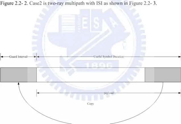
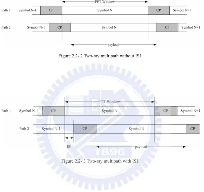
(27) 2.2. Guard Interval. Guard interval is often inserted in the data stream to reduce the inter symbol interference caused by multipath propagation [15]. Guard interval is using constructed with cyclic prefix. The OFDM symbol with guard interval is shown in Figure 2.2- 1. Generally, the length of guard interval should be longer than RMS delay spread of the channel. ISI only damages the information within guard interval. Since the signal is transmitted over multipath channel, the received signal may contain some delayed replica. We show two cases here. Case1 is two-ray multipath without ISI as shown in Figure 2.2- 2. Case2 is two-ray multipath with ISI as shown in Figure 2.2- 3.. Figure 2.2- 1 OFDM symbol with guard interval. 11.
(28) Figure 2.2- 2 Two-ray multipath without ISI. Figure 2.2- 3 Two-ray multipath with ISI. Note that the component of guard interval can not be inserted with zeros. If we insert zeros within guard interval, the signal will lose orthogonality between every two components of the subcarriers which will result in a large degrade in the system performance after DFT operation. Since cyclic prefix still has non-zero power, system should also increase the transmit power when guard interval is longer. The starting position of FFT window must be set properly to avoid ISI from either previous or next symbol. The possible range to set FFT window is that length between 12.
(29) the starting of guard interval of the longest delay ray and the end of guard interval of preceding wave. The delay of the longest delay ray that can avoid ISI is the length of one guard interval. The ideal position for setting FFT window is the beginning of the payload or the end of guard interval of the preceding wave so that the system can admit the longest delay wave. If the symbol timing position is set after the ideal position, ISI with the next symbol occurs, the performance of the receiver is then drastically affected. In summary, the guard interval using cyclic prefix not only preserves the mutual orthogonality between the subcarriers but also prevents the adjacent symbols from ISI. Here we lists the advantages and disadvantage of OFDM [14], [15] and [19] in Table 2.2- 1... Table 2.2- 1 Advantages and disadvantages of OFDM. Advantage. Disadvantage. With symbol and frequency Immunity to delay spread. synchronization problems.. Need FFT units at transmitter and Resistance to frequency selective receiver, higher complexity of fading. computations.. Simple equalization.. Sensitive to carrier frequency offset.. Efficient bandwidth usage.. With high peak-to-average power ratio.. 13.
(30) 14.
(31) Chapter 3 IEEE 802.16e Standard. I. EEE 802.16 standard [2], [3] is for Line-of-Sight (LOS) application, it utilizes 10 Ghz-66 Ghz licensed band. Its channel bandwidths of 25 Mhz or 28 Mhz are typical. With carrier frequency below 11 Ghz, it can support. near-LOS and non-LOS (NLOS), at raw data rate exceeding 120 Mb/s.. 3.1. Overview of WiMAX. Worldwide interoperability for microwave access (WiMAX) is the common name associated to IEEE802.16 standard. WiMAX is also a broadband wireless communication technology designed for high rate data transmission. The application of WiMAX can be applied in DSL, cable modem and so on. WiMAX does not need lots of wiring cost, and it can support wide range wireless service. WiMAX shows great. 15.
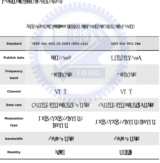
(32) promise as the “last-mile” solution for bringing high-speed internet access into homes and businesses. WiMAX technology has advantages of high data rate and beyond the restriction of terrains, and has the character of mobility. WiMAX was specified in 2003. Intel, Alvarion, Samsung, Fujitsu, Nokia and Siemens all support this standard. IEEE Std. 802.16e is an enhanced version of IEEE Std. 802.16-2004. It can support both fixed and mobile wireless systems, and is compatible with IEEE Std. 802.16-2004. The differences between IEEE Std. 802.16-2004 (802.16d) and IEEE Std. 802.16e are listed in Table 3.1- 1.. Table 3.1- 1 Comparison with IEEE Std.802.16d and IEEE Std. 802.16e. Standard. IEEE Std. 802.16-2004 (802.16d). IEEE Std. 802.16e. Publish date. June, 2004. December, 2005. 2 ~ 66 Ghz. 2 ~ 6 Ghz. Channel. NLOS. NLOS. Data rate. 75 Mbps (bandwidth is 20 Mhz). 15 Mbps (bandwidth is 5 Mhz). Modulation type. BPSK, QPSK, 16-QAM, 64-QAM. BPSK, QPSK, 16-QAM, 64-QAM. bandwidth. 1.5 ~ 20 Mhz. 1.5 ~ 20 Mhz. Mobility. Fixed. Mobile. Frequency band. 16.
(33) The advantages of the WiMAX are summarized as: a.) Suitable in both NLOS and LOS environments. b.) High spectrum efficiency and high data rate. c.) Support the QoS of voice and image.. Due to the cost and complexity associated with traditional wired cable could not provide satisfactory coverage and cause gaps in the broadband coverage, WiMAX is expected to extend the potential of Wi-Fi to far longer distances [1].. 17.
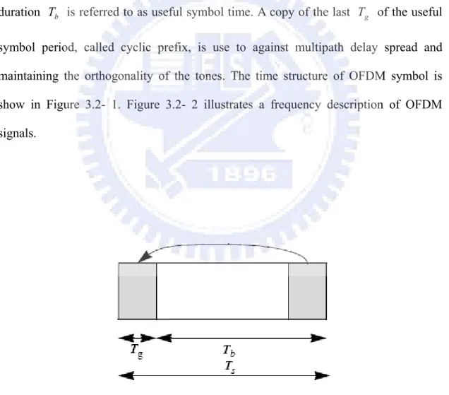
(34) 3.2. WirelessMAN-OFDM PHY. The wirelessMAN-OFDM PHY is based on OFDM modulation and designed for NLOS operation in the frequency bands below 11 Ghz. On initialization, a subscriber station (SS) should search all possible values of cyclic prefix (CP) until it finds the cyclic prefix being used by base station (BS). Once a specific cyclic prefix duration has been selected by the base station for operation on the downlink, it should not be changed. Changing the CP would force all the subscriber stations to resynchronize to the base station. Inverse Fourier transforming creates the OFDM waveform. The time duration Tb is referred to as useful symbol time. A copy of the last Tg of the useful symbol period, called cyclic prefix, is use to against multipath delay spread and maintaining the orthogonality of the tones. The time structure of OFDM symbol is show in Figure 3.2- 1. Figure 3.2- 2 illustrates a frequency description of OFDM signals.. Figure 3.2- 1 Symbol time structure of OFDM. 18.
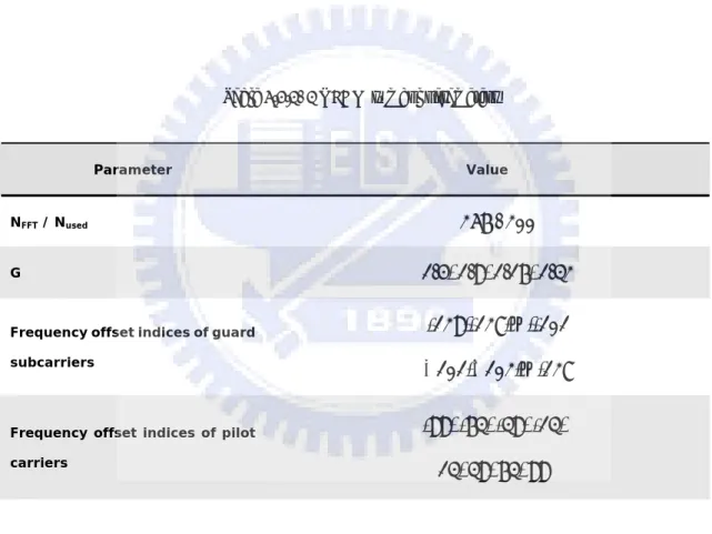
(35) Figure 3.2- 2 Frequency description of OFDM. Data subcarriers: For data transmission. Pilot subcarriers: For various estimation purposes. Null subcarriers: No transmission at all, for guard bands, non-active subcarriers and DC subcarrier.. 3.2.1. OFDM symbol parameters and transmitted signal. Equation (3-1) specifies the transmitted signal voltage to the antenna, as a function of time during any OFDM symbol.. s (t ) = Re{e j 2πf ct ⋅. N used / 2. ∑. ck ⋅ e. j 2πkΔf ( t −Tg ). }. − N used / 2. 19. (3-1).
(36) where t. →. is the time, elapsed since the beginning of the subject OFDM symbol, with 0 < t < Ts .. c k → is a complex number; the data to be transmitted on the subcarrier whose frequency offset index is k, during the subject OFDM symbol. The parameters of the transmitted OFDM signal expressed as Equation (3-1) are given in Table 3.2.1- 1.. Table 3.2.1- 1 OFDM symbol parameters. Parameter. Value. 256 / 200. NFFT / Nused. 1/4, 1/8, 1/16, 1/32. G. -128,-127,…,-101. Frequency offset indices of guard subcarriers. +101,+102,…,127 -88, -63, -38, -13,. Frequency offset indices of pilot carriers. n. 13, 38, 63, 88. For channel bandwidth that are a multiple of:1.75Mhz then n=8/7, 1.5Mhz then n=86/75, 1.25Mhz then n=144/125, 2.75Mhz then n=316/275, 2.0Mhz then n=57/50; otherwise specified then n=8/7.. 20.
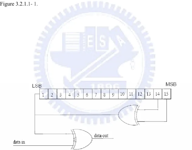
(37) 3.2.1.1. Randomization. Data randomization is performed on each burst of data on the downlink and uplink. The randomization is performed in each data block, the randomizer shall be used independently. If the amount of data to transmit does not fit exactly the amount of data allocated, padding of 0xFF shall be added to the end of the transmission block. The preambles are not randomized, the randomizer sequences is applied only to information bits. A pseudo random binary sequence (PRBS) generator is shown in Figure 3.2.1.1- 1.. Figure 3.2.1.1- 1 PRBS for data randomization. 21.
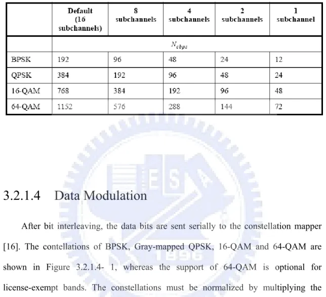
(38) 3.2.1.2 FEC An FEC, consisting of the concatenation of a Reed-Solomon (RS) outer code and a rate-compatible convolutional inner code, are supported on both uplink and downlink. Support BTC and CTC is optional. The BPSK-1/2 should always be used as the coding mode when requesting access to the network and in the FEC burst. The encoding is performed by first passing the data in block format through the RS encoder and then passing it through the zero-terminating convolutional encoder.. 3.2.1.3 Interleaving All encoded data bits are interleaved by a block interleaver with a block size corresponding to the number of coded bits per the allocated subchannels per OFDM symbol. The interlevavr is defined by a two step permutation. The first one ensures that adjacent coded bits are mapped onto nonadjacent subcarriers. The second permutation insures that adjacent coded bits are mapped alternately onto less or more significant bits of the constellation, thus avoiding long runs of lowly reliable bits. Table 3.2.1.3- 1 gives the block size of the bit interleaver.. 22.
(39) Table 3.2.1.3- 1 Block sizes of the bit interleaver. 3.2.1.4. Data Modulation. After bit interleaving, the data bits are sent serially to the constellation mapper [16]. The contellations of BPSK, Gray-mapped QPSK, 16-QAM and 64-QAM are shown in Figure 3.2.1.4- 1, whereas the support of 64-QAM is optional for license-exempt bands. The constellations must be normalized by multiplying the constellation point with the indicated factor c to achieve equal average power. For each modulation, b0 denotes the LSB. The constellation-mapped data must be subsequently modulation onto all allocated data subcarriers in order of increase frequency offset index. The first symbol out of the data constellation mapping should be modulated onto the allocated subcarrier with the lowest frequency index.. 23.
(40) 3.2.2. Preamble structure. All preambles are structured as either one or two OFDM symbol is. The OFDM symbols are defined by the values of composing subcarriers. Each of those OFDM symbols contains a cyclic prefix (CP), which length is the same as the CP for data OFDM symbols. The first preamble consists of two consecutive OFDM symbols. The time domain waveform of the first symbol consists of four repetitions of 64-sample fragment, preceeded by a cyclic prefix (section A). The second OFDM symbol in time domain structure composed of two repetitions of a 128-sample fragment, preceded by a cyclic prefix (section B). The time domain structure are shown in Figure 3.2.2- 1. Figure 3.2.1.4- 1BPSK, QPSK, 16-QAM and 64-QAM constellations 24.
(41) Figure 3.2.2- 1 Downlink and network entry preamble structure. The frequency domain sequences for all full bandwidth preambles are derived form the sequence:. PALL={ 1-j, 1-j, -1-j, 1+j, 1-j, 1-j, -1+j, 1-j, 1-j, 1-j, 1+j, -1-j, 1+j, 1+j, -1-j, 1+j, -1-j, -1-j, 1-j, -1+j, 1-j, 1-j, -1-j, 1+j, 1-j, 1-j, -1+j, 1-j, 1-j, 1-j, 1+j, -1-j, 1+j, 1+j, -1-j, 1+j, -1-j, -1-j, 1-j, -1+j, 1-j, 1-j, -1-j, 1+j, 1-j, 1-j, -1+j, 1-j, 1-j, 1-j, 1+j, -1-j, 1+j, 1+j, -1-j, 1+j, -1-j, -1-j, 1-j, -1+j, 1+j, 1+j, 1-j, -1+j, 1+j, 1+j, -1-j, 1+j, 1+j, 1+j, -1+j, 1-j, -1+j, -1+j, 1-j, -1+j, 1-j, 1-j, 1+j, -1-j, -1-j, -1-j, -1+j, 1-j, -1-j, -1-j, 1+j, -1-j, -1-j, -1-j, 1-j, -1+j, 1-j, 1-j, -1+j, 1-j, -1+j, -1+j, -1-j, 1+j, 0, -1-j, 1+j, -1+j, -1+j, -1-j, 1+j, 1+j, 1+j, -1-j, 1+j, 1-j, 1-j, 1-j, -1+j, -1+j, -1+j, -1+j, 1-j, -1-j, -1-j, -1+j, 1-j, 1+j, 1+j, -1+j, 1-j, 1-j, 1-j, -1+j, 1-j, -1-j, -1-j, -1-j, 1+j, 1+j, 1+j, 1+j, -1-j, -1+j, -1+j, 1+j, -1-j, 1-j, 1-j, 1+j, -1-j, -1-j, -1-j, 1+j, -1-j, -1+j, -1+j, -1+j, 1-j, 1-j, 1-j, 1-j, -1+j, 1+j, 1+j, -1-j, 1+j, -1+j, -1+j, -1-j, 1+j, 1+j, 1+j, -1-j, 1+j, 1-j, 1-j, 1-j, -1+j, -1+j, -1+j, -1+j, 1-j, 1-j, -1-j, 1-j, -1+j, -1-j, -1-j, 1-j, -1+j, -1+j, -1+j, 1-j, -1+j, 1+j, 1+j, 1+j, -1-j, -1-j, -1-j, -1-j, 1+j, 1-j, 1-j }. 25.
(42) The frequency domain sequences for the 4 × 64 sequence, P4×64 , is defined by Equation (3.2.2-1), and 2 × 128 sequences, PEVEN , is defined by Equation (3.2.2-2), where factor. 2 equates the Root-Mean-Square power with that of the data section.. And the additional factor of. 2 is related to the 3-dB boost.. P4×64 (k ) = 2 ⋅ 2 ⋅ conj ( PALL (k )). k mod = 0. P4×64 (k ) = 0. k mod ≠ 0. PEVEN (k ) = 2 ⋅ PALL (k ). k mod 2 = 0. PEVEN (k ) = 0. k mod 2 ≠ 0. 3.2.3. (3.2.2-1). (3.2.2-2). Frame Structure. In licensed bands, the duplexing method must be either TDD or FDD. In license-exempt bands, the duplexing method should be TDD. The OFDM PHY supports a frame-based transmission. A frame consists of a downlink subframe and an uplink subframe. A downlink subframe consists of only one downlink PHY PDU. An uplink subframe consists of contention intervals scheduled for initial ranging and bandwidth request purposes and one or more multiple uplink PHY PDUs, each transmitted from a different subscriber station.. 26.
(43) A downlink PHY PDU starts with a long preamble, which is used for PHY synchronization. The preamble is followed by a FCH burst. The FCH burst is one OFDM symbol long and is transmitted using BPSK rate 1/2. The FCH contains downlink frame prefix to specify burst profile and length of one or several downlink bursts immediately following the FCH. The FCH is followed by one or more multiple downlink bursts, each transmitted with different burst profile. Each downlink burst consists of an integer number of OFDM symbols. With the OFDM PHY, a PHY burst, either a downlink PHY burst or an uplink PHY burst, consists of an integer number of OFDM symbols, carrying MAC messages. To from an integer number of OFDM symbols, unused bytes in the burst payload maybe padded by the bytes 0xFF. In each time division duplex or duplexing (TDD) frame, see Figure 3.2.3- 1, the TTG and RTG must be inserted between the downlink and uplink subframe and at the end of each frame, respectively, to allow the base station (BS) to turn around. The downlink and uplink frame structure of FDD of an OFDM system are shown in Figure 3.2.3- 2 .. 27.
(44) Figure 3.2.3- 1 Example of OFDM frame structure with TDD. 28.
(45) Figure 3.2.3- 2 Example of OFDM frame structure with FDD. 29.
(46) 30.
(47) Chapter 4 Frame Synchronization Techniques. O. FDM is a kind of multi-carrier modulation on multi-channel. By adding guard interval (GI) between OFDM symbols, OFDM WLAN system can be against multipath delay spread. Signals can be detected. up on the reception of just one training sequence of two OFDM symbols. Finding the symbol timing for OFDM means finding an estimate of where the symbol starts. There have been several methods of synchronization for OFDM in recent years [4]-[6], [17] and [22]. Some new schemes has been proposed in [18]-[21], they use the convolution characteristic of cyclic prefix to overcome the defects of the fluctuation of the estimated start position. In this chapter, we will introduce Schmidl & Cox algorithm [10] and Feng Lu, et al.’s adaptive symbol timing (AST) algorithm [11], which try to overcome the fault of plateau in Schmidl & Cox’s algorithm of the fluctuation of the estimated start position. 31.
(48) Finally, we will introduce the pseudo-multipath iteration algorithm (PMIA) [12], which provide a new concept of pseudo-multipath.. 4.1 System Architecture Figure 4.1- 1 is the system architecture of OFDM system. It shows the action between Transceiver (Tx) and receiver (Rx). Transceiver deliver signals to receivers through radio channel. As for the channel model, we use SUI channel model, see section 4.1.1. Signals from transceivers may distort because of channel fading or delay spread. We must create some mechanism to recover the correct timing so as to let receivers receive the correct signals form transceivers. Because of not knowing the correct timing for signals, we must detect the exact timing of signals of the receivers for synchronization. If the timing of these signals can not synchronized, the signal may either produce phase rotation or cause errors on the received signals. Therefore, synchronization at the receiver is one important step that must be performed.. 4.1.1 SUI Channel Model As for the channel model, we would like to construct SUI channel, taking SUI parameters in reference document 802.16.3c01-29r4 [7]. Because the system is designed for NLOS environment, we use Jakes model accompanied with SUI channel parameters to build this fading channel [8], [9].. 32.
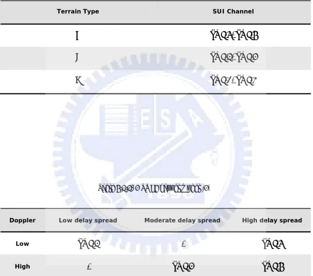
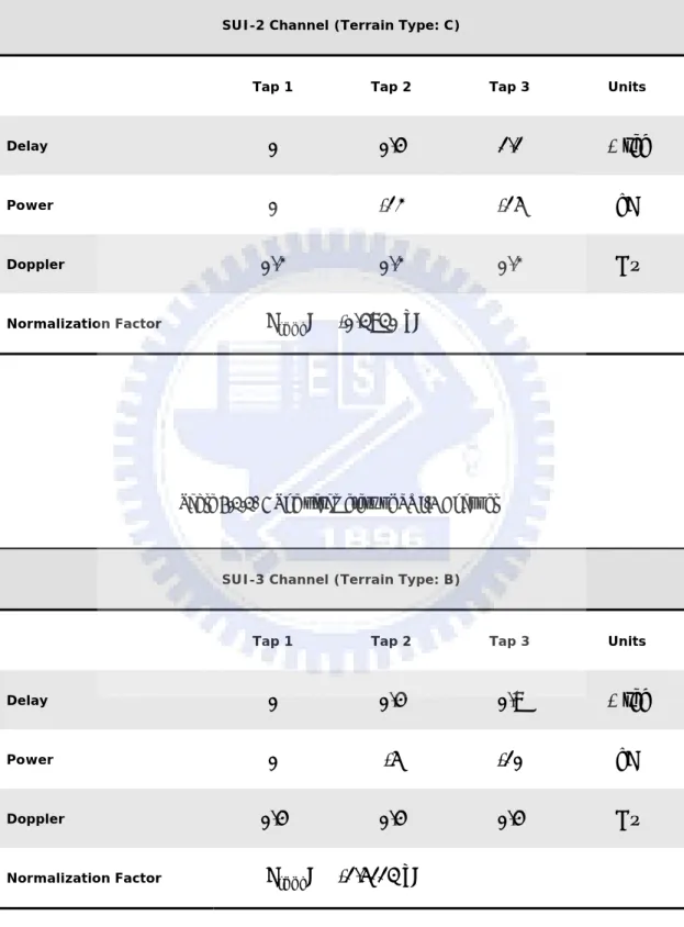
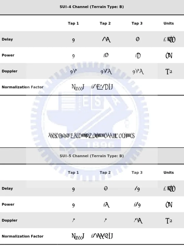
(49) Figure 4.1- 1 802.16-2004 System Structure. The SUI model defines three types of terrains, given below: Category A: maximum path loss, hilly terrain, moderate-to-heavy tree density. Category B: Intermediate path loss, flat terrain, light tree density. Category C: minimum path loss, flat terrain, light tree density. These categories are shown in Table 4.1.1- 1 and Table 4.1.1- 2. Figure 4.1.1- 1 shows examples for each taps magnitude. We list all of the SUI channel parameters in Table 4.1.1- 3 to Table 4.1.1- 8 that will be used in our simulations below.. 33.
(50) Table 4.1.1- 1 SUI Channel model (1). Terrain Type. SUI Channel. A. SUI-5, SUI-6. B. SUI-3, SUI-4. C. SUI-1, SUI-2. Table 4.1.1- 2 SUI Channel model (2). Doppler. Low delay spread. Moderate delay spread. High delay spread. Low. SUI-3. -. SUI-5. High. -. SUI-4. SUI-6. 34.
(51) Figure 4.1.1- 1 An example of tap fading of SUI-3 Channel. Table 4.1.1- 3 The parameters of SUI-1 Channel. SUI-1 Channel (Terrain Type: C). Tap 1. Tap 2. Tap 3. Units. Delay. 0. 0.4. 0.9. μ sec. Power. 0. -15. -20. dB. 0.4. 0.4. 0.4. Hz. Doppler. Normalization Factor. Fommi =. -0.1771 dB. 35.
(52) Table 4.1.1- 4 The parameters of SUI-2 Channel. SUI-2 Channel (Terrain Type: C). Tap 1. Tap 2. Tap 3. Units. Delay. 0. 0.4. 1.1. μ sec. Power. 0. -12. -15. dB. 0.2. 0.2. 0.2. Hz. Doppler. Normalization Factor. Fommi = -0.3930 dB. Table 4.1.1- 5 The parameters of SUI-3 Channel. SUI-3 Channel (Terrain Type: B). Tap 1. Tap 2. Tap 3. Units. Delay. 0. 0.4. 0.9. μ sec. Power. 0. -5. -10. dB. 0.4. 0.4. 0.4. Hz. Doppler. Normalization Factor. Fommi =. -1.5113 dB. 36.
(53) Table 4.1.1- 6 The parameters of SUI-4 Channel. SUI-4 Channel (Terrain Type: B). Tap 1. Tap 2. Tap 3. Units. Delay. 0. 1.5. 4. μ sec. Power. 0. -4. -8. dB. 0.2. 0.15. 0.25. Hz. Doppler. Normalization Factor. Fommi =. -1.9218 dB. Table 4.1.1- 7 The parameters of SUI-5 Channel. SUI-5 Channel (Terrain Type: B). Tap 1. Tap 2. Tap 3. Units. Delay. 0. 4. 10. μ sec. Power. 0. -5. -10. dB. Doppler. 2. 2. 2.5. Hz. Normalization Factor. Fommi =. -1.5513 dB. 37.
(54) Table 4.1.1- 8 The parameters of SUI-6 Channel. SUI-6 Channel (Terrain Type: B). Tap 1. Tap 2. Tap 3. Units. Delay. 0. 14. 20. μ sec. Power. 0. -10. -14. dB. 0.4. 0.4. 0.4. Hz. Doppler. Normalization Factor. Fommi =. -0.5683 dB. In accordance with IEEE Std. 802.16e in reference [3], we modify the SUI channel model. We only adjust the parameters with Doppler frequency [13]. In 2.5 Ghz licensed band, 7 Mhz bandwidth and 120 km/hr to calculate the Doppler frequency, and then modify the tap magnitude of each SUI channel parameters. We can see the detail equations and its computing procedure in the section 5.2.. 38.
(55) 4.1.2 Simulation Parameters Table 4.1.2- 1 lists the parameters and its value that we used in our fixed and mobile simulations [12].. Table 4.1.2- 1 System Simulation Parameters. Parameter. Value. Number of subcarrier (N). 256 (include 200 used subcarriers). Pilot Number (P). 8. Bandwidth (BW). 7 Mhz / (10 Mhz for licensed-exempt band). Carrier spacing ( Δf ). 31.25 Khz. Sampling Rate (. fs ). 8 Mhz / (11 Mhz for licensed-exempt band). Symbol Rate. 25 Khz. Mapping Modulation. 16-QAM. Useful Time. 32μsec. Cyclic Prefix. 1/4. OFDM symbol time. 40μsec. Frequency offset (Normalized). 0.25. 39. (256 samples). (320 samples).
(56) 4.2 Some Frame Synchronization Algorithms Symbol timing error will affect the amplitude of the received signal and carrier phase. It also introduces ISI. In order to correctly demodulate the signal, we must find the start point of OFDM symbol before FFT demodulation.. 4.2.1. Schmidl & Cox Algorithm. In 1997, Schmidl & Cox [10] introduced a technique employing the preamble to estimate the start point of the received OFDM signal. However, the outcome produces a plateau in metric function. This plateau leads to some uncertainty in the estimated start position. We list the timing metric functions of Schmidl & Cox method for frame timing estimation below:. L −1. P(d ) = ∑ rd*+ m ⋅ rd + m + L. (4.2.1-1). m =0 L −1. R (d ) = ∑ rd + m + L. 2. (4.2.1-2). m =0. M (d ) =. P(d ). 2. (4.2.1-3). [ R(d )]2. where L=128. 40.
(57) Figure 4.2.1- 1 shows the block diagram of Schmidl & Cox algorithm. Schmidl & Cox algorithm has a plateau region, the result of single frame simulation as shown in Figure 4.2.1- 2. We still can find a maximum value in this region. The position of maximum value is used as the start point of the OFDM symbol.. Figure 4.2.1- 1 Block diagram of Schmidl & Cox algorithm. Figure 4.2.1- 2 Schmidl & Cox Algorithm (for CP=64, L=128) 41.
(58) 4.2.2.. Adaptive Symbol Timing Algorithm (ASTA). Recently, Feng Lu et al. introduced a new method called adaptive symbol timing (AST) algorithm [11], which used the autocorrelation of the received signal and its delayed version to get frame timing synchronization. The AST algorithm needs a preamble whose length is equal to two OFDM symbols (a section A preamble and a section B preamble). Based on Schmidl & Cox algorithm, by fixing the length of cyclic prefix and the length of correlation window, we can find the first peak at the end of the section A preamble. Then, we can find another peak at the end of the section B preamble. Then, we can find the only peak by the mean value of the metric function M(k) and the metric function M (k − 320) and divided by two, see Equation (4.2.2-4). All timing metric functions are shown in Equations (4.2.2-1), (4.2.2-2), (4.2.2-3) and (4.2.2-4). Finally, we can get the peak value. The position of the peak value is defined as the start point of the symbol.. N −1. P (k ) = ∑ r (k + i ) ⋅ r * (k + Td 1 + i ). (4.2.2-1). i =0. N −1. R(k ) = ∑ r (k + i ). 2. (4.2.2-2). i =0. M (k ) =. P(k ) ⋅ P(k ) * ( R (k )) 2. MM (k ) =. (4.2.2-3). M (k ) + M (k − Td 2 ) 2. (4.2.2-4). where N=192, Td 1 = 128 Td 2 = 320. 42.
(59) Note that, N is the length of correlation window. Figure 4.2.2- 1 shows the block diagram of AST algorithm. After ASTA operation, we will not find the plateau as that in using Schmidl & Cox algorithm anymore and get a unique peak in curve of metric function MM(k) [18]. In this way, we have a much better precision in the estimate of start position. The results of single frame simulation of the metric functions MM(k) and M(k) are shown in Figure 4.2.2- 2.. Figure 4.2.2- 1 Block diagram of AST algorithm. 43.
(60) Figure 4.2.2- 2 AST Algorithm. In a wireless environment, signals may have fading and multipath delay spread when passing the channels. Figure 4.2.2- 3 is the probability distribution of estimated start positions of 20000 frames. However, the more precise ratio in the estimation by using AST algorithm would just be 61.8% at time error index 0 [12], as shown in Figure 4.2.2- 3.. 44.
(61) Figure 4.2.2- 3 The estimate probability distribution in SUI-3 of AST Algorithm. 4.2.3. Pseudo-Multipath Iteration Algorithm (PMIA). In 2005, C. C. Wu [12] in his thesis introduced a concept of pseudo multipath. The scheme is based on the AST algorithm. First, the algorithm defined a pseudo path with preamble which is two-OFDM symbol long (a section A preamble and a section B preamble). We can get a unique peak at the end of the preamble. Then, we exploit the peak index for the start position of the pseudo path that we want to insert in. We would use the original signal added with a preamble multiplied a factor α, and moves forward in time frame by λ. This outcome is seen as original signal with a pseudo-path. In the 45.
(62) same way, we must iterate several times to get the final outcome of the PMIA algorithm. After several times of iteration, the peak’s position of the last iteration will then become our estimated start position. The PMIA algorithm can further increase the precision of the estimation of start position. In PMIA, three variables must be set: 1) the strength of pseudo path, 2) the timing of pseudo path inserted and 3) times of iteration. Because there are three variables that should be optimized, it is difficult to get the trade off among these variables. The PMIA needs a lot of computation complexity for the iterative operation, and need more hardware for the computation. Although PMIA has some disadvantages but it still has advantages. The PMIA is not only more precise than AST algorithm but also able to fine-tune the system performance when we select a smaller value of α. The timing of inserting the pseudo path in PMIA is shown in Figure 4.2.3- 1. From the computer simulation results within the thesis [12], we can see that the optimized value of these parameters in fixed SUI-3 environment is: α=0.1, λ=6 and 4 times of iteration. We will show our computer simulation results using the same optimized value [12] as listed above and compare the system performance with PMIA and PMA in fixed SUI-3 environment as shown in the section 5.1.1.. 46.
(63) Figure 4.2.3- 1 The timing of pseudo path inserted for AST algorithm. 47.
(64) 48.
(65) Chapter 5 Modified Pseudo-Multipath Algorithm. I. n this chapter, we will present a new method by putting a section B preamble in the receiver when we use the pseudo-path for the frame timing synchronization. This modified pseudo multipath algorithm. (PMA) can increase the accuracy of frame timing estimation without adding more hardware. We apply this method in TDD, downlink OFDM system which fits IEEE 802.16-2004/e Std. environment [2], [3].. 5.1 Modified Pseudo-Multipath Algorithm (PMA) To increase the precision of estimation of the start position, we apply the concept of pseudo-multipath [12]. The pseudo multipath algorithm uses a section B preamble in the receiver as a pseudo-multipath (4th tap) shown in Figure 3.2.2- 1. First, we exploit a. 49.
(66) section A preamble of the original signal to find the position of the first peak of M(k) curve, see Equation (4.2.2-3). Then, we put a section B preamble prior to the first peak whose length is λ, and used it as a pseudo-path. This section B preamble multiplied by a factor α, then adds the original signal to become a new received signal for following calculation. Then we can find the only peak on the curve of MM(k), and the position of the peak is defined as the symbol start position. The block diagram is shown in Figure 5.1- 1. In Figure 5.1- 1, the green part shows the differences between pseudo multipath algorithm and AST algorithm. We just add only a set of adder and one multiplexer. In Figure 5.1- 1, the multiplier is replaced by a bit shifter to save a set of multiplier. Therefore, we limit our value of the factor α to 2 n where n can be any positive or negative integer, including 0. We select the value of the factor α as 1, 0.5, 0.25 and 0.125 in our hardware design. We also show PMA algorithm flow chart in Figure 5.1- 2. In the proposed scheme (PMA), we will increase the precision of estimation of the start position and eliminate a variable of times of iteration of the PMIA. The PMA only uses a section B preamble in the receiver (note that: PMIA needs a section A preamble and a section B preamble in the receiver) and reduce the hardware and computation complexity successfully. The following equation tells us how the pseudo multipath can be used to fight against channel delay spread [12]. Equation (5.1-1) is the outcome of the auto-correlation of the received signal. When h1 result of auto-correlation will be dominated by h1 2. 2. 2. 2. is much larger than h2 . The term. Also, when h2. larger than h1 , the result of auto-correlation will be dominated by h2. 2. 2. is much. term. This. also means that the estimated start position is mainly influenced by one of the taps of multipath. Note that: noise term is not considered in the following computation. 50.
(67) Figure 5.1- 1 Block Diagram of PMA algorithm. 192. f (d ) = ∑ ri + d ri*+ d −128 i =1. 192. = ∑ {(h1 xi + d + h2 xi + d +τ1 + h3 xi + d +τ 2 )(h1 xi + d −128 + h2 xi + d +τ1 −128 + h3 xi + d +τ 2 −128 ) * } i =1. 192. = ∑ { h1 xi + d xi + d −128 + h1 h2* xi + d xi*+ d +τ 1 −128 + h1 h3* xi + d xi*+ d +τ 2 −128 + 2. i =1. 2. h1* h2 xi + d +τ 1 xi*+ d −128 + h2 xi + d +τ1 xi*+ d +τ1 −128 + h2 h3* xi + d +τ1 xi*+ d +τ 2 −128 + 2. h1* h3 xi + d +τ 2 xi*+ d −128 + h2* h3 xi + d +τ 2 xi*+ d +τ 1 −128 + h3 xi + d +τ 2 xi*+ d +τ 2 −128 }. 51.
(68) 192. = ∑ ( h1 xi + d xi*+ d −128 + h2 xi + d +τ1 xi*+ d +τ1 −128 + h3 xi + d +τ 2 xi*+ d +τ 2 −128 ) 2. 2. 2. i =1. (5.1-1). From Equation (5.1-1), we can easily find that the outcome signal f (d ) is the auto-correlation sum of the original signal passing through the channel with some fading and delay. Similarly, α is a factor multiplying the pseudo-path to define its influence on the original signal. Then, we use λ to set the position of the influence of pseudo-path, adding with the original signal, and produce a new signal. Figure 5.1- 3 shows the timing of pseudo-path, and Equation (5.1-2) shows the outcome of adding pseudo-path, and ε is the offset between the first estimated peak from the timing metric M(k) and the ideal peak position of the timing metric M(k). Noise term is still not considered here.. 192. f (d ) = ∑ ri + d ri*+ d −128 i =1. 192. = ∑ {(h1 xi + d + h2 xi + d +τ 1 + h3 xi + d +τ 2 + αxi + d +ε −λ )(h1 xi + d −128 + h2 xi + d +τ1 −128 + i =1. h3 xi + d +τ 2 −128 + αxi + d +ε −λ −128 ) * } 192. f (d ) ≅ ∑ { h1 xi + d xi + d −128 + h2 xi + d +τ1 xi + d +τ1 −128 + h3 xi + d +τ 2 xi*+ d +τ 2 −128 + 2. 2. 2. i =1. α 2 xi + d +ε −λ xi*+ d +ε −λ −128 } (5.1-2). 52.
(69) Therefore, when the value of α 2 is large, this equation may be dominated by the. α 2 term (pseudo-path term), which means that the signal will be dominated by pseudo multipath. If the value of each term is similar, the outcome would be the sum of each term, not dominated by any single term. We use Equation (5.1-3) and Equation (5.1-4) to evaluate the system performance (the deviation of the frame start point) in either fixed or mobile environments.. ∑ (estimation _ index − ideal _ index). Estimate index RMS =. No _ Frame. No _ Frame. 2. (5.1-3). ∑ (estimation _ index − ideal _ index). Estimate index Mean =. No _ Frame. No _ Frame. 53. (5.1-4).
(70) Figure 5.1- 2 Flow chart of PMA. 54.
(71) Figure 5.1- 3 Timing of pseudo-path insert. 55.
(72) Next, we simulate 20000 frames, at SNR=5dB to SNR=30dB in SUI-3 channel environment. In Figure 5.1- 4 and Figure 5.1- 5, we show the system performance of PMA compared with normal mode (ASTA mode) when the system is in the AWGN channel. Then, we try to set different values of α and λ in the SUI-3 channel to examine the variations of system performance by different values of α and λ. We limit the value of α to be 1, 0.5, 0.25 or 0.125, to avoid the use of multiplier. We only show the optimized λ value in each α that we found from Figure 5.1- 7 to Figure 5.1- 15. Then, we can get the optimized value of α and λ in SUI-3 channel environment. From the result of the previous description and simulation, we find that α=0.5 and λ=33 is the optimized value in SUI-3 environment for IEEE Std. 802.16-2004. Because its RMS value and mean value are closer to the center than other combinations of α and λ, it indicates that the average estimated start position of every frame is very close to the ideal start position of frames. Figure 5.1- 16 shows the system performance when α=0.5 and λ=33, and it also shows the comparison with timing error probability distribution between normal mode and PMA mode at 10dB SNR and 30dB SNR. These results are shown in Figure 5.1- 17 and Figure 5.1- 18. From the result of computer simulations, we can find that the PMA’s system performance is much better than AST algorithm without pseudo path. It also shows that pseudo multipath algorithm apparently makes the estimated start position much closer to the center (which is the ideal start position; that is, index 0 as shown in Figure 5.1- 17 and Figure 5.1- 18).. 56.
(73) Figure 5.1- 4 RMS of PMA mode in AWGN channel (α=0.5, λ=0). Figure 5.1- 5 Mean of PMA mode in AWGN channel (α=0.5, λ=0) 57.
(74) RMS (SUI-3):. Figure 5.1- 6 RMS PMA mode in SUI-3 channel (α=1). Figure 5.1- 7 RMS PMA mode in SUI-3 channel (α=0.5) 58.
(75) Figure 5.1- 8 RMS PMA mode in SUI-3 channel (α=0.25). Figure 5.1- 9 RMS PMA mode in SUI-3 channel (α=0.125) 59.
(76) Mean (SUI-3):. Figure 5.1- 10 Mean PMA mode in SUI-3 channel (α=1). Figure 5.1- 11 Mean PMA mode in SUI-3 channel (α=0.5) 60.
(77) Figure 5.1- 12 Mean PMA mode in SUI-3 channel (α=0.25). Figure 5.1- 13 Mean PMA mode in SUI-3 channel (α=0.125) 61.
(78) Comparison (SUI-3):. Figure 5.1- 14 PMA mode in SUI-3 channel (RMS). Figure 5.1- 15 PMA mode in SUI-3 channel (Mean) 62.
(79) Figure 5.1- 16 RMS and Mean of PMA mode in SUI-3 channel (α=0.5, λ=33). 63.
(80) Figure 5.1- 17 Time Error at SNR=10dB of PMA mode in SUI-3 channel (α=0.5, λ=33). Figure 5.1- 18 Time Error at SNR=30dB of PMA mode in SUI-3 channel (α=0.5, λ=33). 64.
(81) The green line sets α=0 and λ=0, that is, the system works using AST algorithm. In this mode, the system without pseudo path is called “Normal Mode” in our simulations. The blue line shows the system performance after adding pseudo path. From the results of simulations, we see that PMA algorithm can improve system performance a lot. In the same way, when we find the optimized value of α and λ in SUI-3, we put the same parameters α and λ in the other SUI channels (SUI-1/SUI2 and SUI-4 to SUI-6 environments), to check if it can improve the system’s performance. Figure 5.1- 19 to Figure 5.1- 23 show the system performance when we set α=0.5 and λ=33 (the optimized value at SUI-3 channel) in different SUI channels.. Figure 5.1- 19 SUI-1 (α=0.5, λ=33 ). 65.
(82) Figure 5.1- 20 SUI-2 (α=0.5, λ=33 ). Figure 5.1- 21 SUI-4 (α=0.5, λ=33 ) 66.
(83) Figure 5.1- 22 SUI-5 (α=0.5, λ=33 ). Figure 5.1- 23 SUI-6 (α=0.5, λ=33 ) 67.
(84) From the result of the simulations, we find the fact that the same set of parameters can not be suit to every SUI environment. To further analyze the result, we can find that the Doppler shift and tap’s power of each multipath of SUI-1 and SUI-2, respectively, are weaker than other SUI channels. This means that in the SUI-1 and SUI-2 environments, signals are transmitted in a good channel environment. Therefore, if we add a pseudo-path, its strength and the length moved forward by λ would be the same as that in SUI-3 channel. It does not improve or degrade the performance of the estimated start position. But if the system is in a serious multipath delay spread environment, we can improve the estimation accuracy a lot by adding the pseudo path. How do we solve the problems that the system performance may be degraded in SUI-1 and SUI-2 channels by using PMA? First, we use a few frames at the start of bursts and set α=0 and λ=0 to detect the current system channel environment. By the result of detection, the system will figure out the current channel environment. Then we switch to PMA mode and dynamically set the new α and λ values that are suitable for the channel. This procedure can work periodically when we need. We can get better system performance than ASTA mode after training. The same procedure can be applied to either fixed or mobile environment. We care about the individual optimized value of α and λ in the different SUI channels. Next, we will show the computer simulation results to see the optimized values of α and λ in SUI-1, SUI-2, SUI-4, SUI-5 and SUI-6 as shown in Figure 5.1- 24 to Figure 5.1- 33.. 68.
(85) Figure 5.1- 24 SUI-1 (RMS). Figure 5.1- 25 SUI-1 (Mean) 69.
(86) Figure 5.1- 26 SUI-2 (RMS). Figure 5.1- 27 SUI-2 (Mean) 70.
(87) Figure 5.1- 28 SUI-4 (RMS). Figure 5.1- 29 SUI-4 (Mean) 71.
(88) Figure 5.1- 30 SUI-5 (RMS). Figure 5.1- 31 SUI-5 (Mean) 72.
(89) Figure 5.1- 32 SUI-6 (RMS). Figure 5.1- 33 SUI-6 (Mean) 73.
(90) Table 5.1- 1 Optimization parameter of IEEE Std. 802.16d. SUI-1. SUI-2. SUI-3. SUI-4. SUI-5. SUI-6. α. 0.25. 0.5. 0.5. 1. 1. 0.5. λ. 26. 26. 33. 0. 32. 14. From the result of all the above mentioned, we list the recommended individual optimized values of α and λ in each SUI channel, as shown in Table 5.1- 1.. 5.1.1. Comparison of PMA with Schmidl & Cox Algorithm and PMIA. In the previous section, we have introduced Schmidl & Cox algorithm [10]. Now, if we put the system in the same SUI environment (SUI-3) and set the system parameter as α=0.5 and λ=33 in PMA mode, and then compare the performance of PMA mode and that of Schmidl & Cox algorithm. The performances are shown in Figure 5.1.1- 1 and Figure 5.1.1- 2. We also compare the performance of PMIA and PMA. The results are shown in Figure 5.1.1- 3 and Figure 5.1.1- 4. From the result of the simulations, we can see that PMA algorithm is much better than Schmodl & Cox algorithm and PMIA on frame-timing estimate.. 74.
(91) Figure 5.1.1- 1 Schmidl & Cox vs. PMA in fixed SUI-3 (RMS). Figure 5.1.1- 2 Schmidl & Cox vs. PMA in fixed SUI-3 (Mean) 75.
(92) Figure 5.1.1- 3 ASTA and PMIA vs. PMA in fixed SUI-3 (RMS). Figure 5.1.1- 4 ASTA and PMIA vs. PMA in fixed SUI-3 (Mean) 76.
(93) We compare all the algorithms we introduced above including precision of the estimated start position of signals, the complexity of computations and the complexity of hardware [23]. The results are summarized as: 1) Precision of estimation: PMA > PMIA > ASTA >> Schmidl & Cox. 2) Complexity of computation: PMIA >> PMA = ASTA ≅ Schmidl & Cox. 3) Hardware complexity: PMIA >> PMA ≅ ASTA ≅ Schmidl & Cox.. By comparing the computation complexity and hardware complexity, PMIA has the highest effort and the effort of Schmidl & Cox, ASTA and PMA algorithms are very similar. But PMA has the highest precision of estimated start position among all the algorithms.. Table 5.1.1- 1 Comparison of PMA with Schmidl & Cox Algorithm and PMIA. Schmidl & ASTA. PMIA. PMA. Cox Precise of estimation. Low. High. High. The Highest. Complexity of computation. Low. Low. The Highest. Low. Hardware complexity. Low. Low. The Highest. Low. 77.
(94) 5.2 IEEE 802.16e System All the above simulations fit IEEE Std. 802.16-2004 OFDM PHY specification [2]. If we put PMA in mobile environment to fit IEEE Std. 802.16e [3], what influence it might have on the system performance? By reference [13], we rebuild the channel model for mobile environment, and set the system to work in 2.5GHz band, mobile velocity at 120km/hr. We use Equation (5.2-1) to calculate the corresponding Doppler frequency, and obtain 277.8 hz.. fD =. v × f c × cos θ c. (5.2-1). where v=120km/hr, c = 3× 10 8 m/s, θ = 0 o. fD =. 120 × 1000 × (1 /(60 × 60) ) × 2.5 × 10 9 × cos(0) 8 3 × 10. = (1.11 × 10 −7 ) × (2.5 × 10 9 ) × 1 = 277.777 Hz. After rebuilding the channel in mobile environment, the system performances from software simulations are shown in Figure 5.2- 1 to Figure 5.2- 12.. 78.
(95) Figure 5.2- 1 Mobile SUI-1 RMS. Figure 5.2- 2 Mobile SUI-1 Mean 79.
(96) Figure 5.2- 3 Mobile SUI-2 RMS. Figure 5.2- 4 Mobile SUI-2 Mean 80.
(97) Figure 5.2- 5 Mobile SUI-3 RMS. Figure 5.2- 6 Mobile SUI-3 Mean 81.
(98) Figure 5.2- 7 Mobile SUI-4 RMS. Figure 5.2- 8 Mobile SUI-4 Mean 82.
(99) Figure 5.2- 9 Mobile SUI-5 RMS. Figure 5.2- 10 Mobile SUI-5 Mean 83.
(100) Figure 5.2- 11 Mobile SUI-6 RMS. Figure 5.2- 12 Mobile SUI-6 Mean 84.
(101) From the result, we list the recommended optimized values of α and λ in each SUI channel in Table 5.2- 1. We will investigate if the system works in 3.5 Ghz licensed band, with 7 Mhz bandwidth, or in the other frequency bands and bandwidth.. Figure 5.2- 13 to Figure. 5.2- 20 show the performances when the system is in IEEE Std. 802.16-2004, IEEE Std. 802.16e / 120 km/hr / 2.5 Ghz licensed band, IEEE Std. 802.16e / 120 km/hr / 3.5 Ghz licensed band, with bandwidth is 7 Mhz, and IEEE Std. 802.16e / 120 km/hr / 6 Ghz license-exempt band with bandwidth 10 Mhz in the SUI-3 channel [2] [3].. Table 5.2- 1 Optimization parameter of IEEE Std. 802.16e. SUI-1. SUI-2. SUI-3. SUI-4. SUI-5. SUI-6. α. 0.25. 0.5. 1. 1. 1. 1. λ. 3. 5. 3. 13. 15. 10. 85.
(102) Figure 5.2- 13 802.16d SUI-3 (RMS). Figure 5.2- 14802.16d SUI-3 (Mean) 86.
(103) Figure 5.2- 15802.16e SUI-3 at 2.5 Ghz band (RMS). Figure 5.2- 16802.16e SUI-3 at 2.5 Ghz band (Mean) 87.
(104) Figure 5.2- 17 802.16e SUI-3 at 3.5 Ghz band (RMS). Figure 5.2- 18 802.16e SUI-3 at 3.5 Ghz band (Mean) 88.
(105) Figure 5.2- 19 802.16e SUI-3 at 6 Ghz license-exempt band (RMS). Figure 5.2- 20 802.16e SUI-3 at 6 Ghz license-exempt band (Mean) 89.
(106) From the simulation results listed above, PMA in IEEE Std. 802.16e environment, no matter the system is in 2.5 Ghz licensed band or in 3.5 Ghz licensed band or in 6 Ghz licensed-exempt band, PMA still has better performance than AST algorithm for estimation of start position. Furthermore, when the system is in a severer multipath delay spread environment, we can get the simulation result in the environment that fits IEEE Std. 802.16-2004 or IEEE Std. 802.16e environment. PMA algorithm still can improve the system performance by adjusting the factors α and λ. When signals in the good channel environment, the strength of pseudo-path (the value of α) does not need to be strong to avoid interference of the original signal which already has good quality. We can also use the procedure discussed in section 5.1. The system can select the best parameters. In this technique, we may design a system which is suitable for different SUI channels under fixed or mobile environments.. 90.
(107) 5.3 Fix-Point Simulation Because of the limit of chip area and routing complexity, and other problems, we often avoid implementing VLSI circuit by floating paint data format in the real world. Generally, if we use finite numbers of bits in implementation of the chip, and if its result is very close to that of using floating-point data format, we can choose finite-bit format to implement on VLSI. In this way, we can save not only chip area but also routing complexity, and thus decrease the cost. Next, engineers must find how many bits we implement in real chips and make system performance close to the result of floating-point.. Figure 5.3- 1 Fix-Point structure. 91.
(108) The fix-point data format is shown in Figure 5.3- 1. In the transmitter, the power of transceiver signal must be quantized and normalized. No matter what kind of modulation types, its real part and imaginary part are smaller than one after normalization. The maximum value of the transmitted signal will be in the preamble before IFFT. On the effect of signal passing through the channel, the amplitude value of signals may become larger in the receiver. Its value may be larger than three [12], [16]. Therefore, we use three bits to express the integer part. The MSB is the sign bit. The reminding part is used to express the decimal part. The precision of the quantization depends on how many quantization bits that we use. In fix-point simulation, in the circled dash line, the indexed position shows the part that MATLAB program must do the floating-point to fix-point translation, see Figure 5.3- 2. Before the signals are transmitted from the transmitter, we translate floating-point data format to fix-point data format in our programs. In a similar way, signals from the channel will also be translated from floating-point data format to fix-point data format in our program. When we simulate in fix-point data format, we simulate both truncation mode and rounding mode to see the results when we use different translation data formats. The simulation result of rounding mode are shown in Figure 5.3.1- 1 and Figure 5.3.1- 2, and the results of truncation mode are shown in Figure 5.3.2- 1 and Figure 5.3.2- 2.. 92.
(109) Figure 5.3- 2 The floating-point to fix-point position in system. 93.
(110) 5.3.1 Rounding Mode. Figure 5.3.1- 1 Rounding Mode in SUI-3 channel (RMS). Figure 5.3.1- 2 Rounding Mode in SUI-3 channel (Mean) 94.
(111) 5.3.2. Truncation Mode. Figure 5.3.2- 1 Truncation Mode in SUI-3 channel (RMS). Figure 5.3.2- 2 Truncation Mode in SUI-3 channel (Mean) 95.
(112) We can get the same results of computer simulation of truncation and rounding mode, the result of fix-point simulation is consistent with floating-point simulation when we use 14-bit word length. In fix-point simulation, even in the different floating-point to fix-point translation mode (rounding mode or truncate mode), we can see that no matter what kind of translation format, we can get the same outcome: we can use 14-bit to implement our system in VLSI circuit, and the system performance is very close to floating-point system performance as we simulate in the computer. Therefore, 14-bit word length is recommended to implement the system on VLSI circuit.. 96.
數據
+7
相關文件
This thesis applied Q-learning algorithm of reinforcement learning to improve a simple intra-day trading system of Taiwan stock index future. We simulate the performance
In this chapter, we have presented two task rescheduling techniques, which are based on QoS guided Min-Min algorithm, aim to reduce the makespan of grid applications in batch
In this thesis, we have proposed a new and simple feedforward sampling time offset (STO) estimation scheme for an OFDM-based IEEE 802.11a WLAN that uses an interpolator to recover
In this thesis, we propose a Density Balance Evacuation Guidance base on Crowd Scatter Guidance (DBCS) algorithm for emergency evacuation to make up for fire
This is to inform kindergartens and primary schools of the “Library Cards for All School Children” scheme and the arrangement of bulk application for library cards of the
In this talk, we introduce a general iterative scheme for finding a common element of the set of solutions of variational inequality problem for an inverse-strongly monotone mapping
At least one can show that such operators has real eigenvalues for W 0 . Æ OK. we did it... For the Virasoro
In this study, we compute the band structures for three types of photonic structures. The first one is a modified simple cubic lattice consisting of dielectric spheres on the
