電子工程學系 電子研究所
碩士論文
應用於單載波室內無線接收器之快速適應頻率域通道
等化器之設計
Design of Fast Convergent Adaptive
Frequency-Domain Equalizer for Single Carrier
Indoor Wireless Receiver
研 究 生:劉代暘
指導教授:周世傑 教授
頻率域通道等化器之設計
Design of Fast Convergent Adaptive
Frequency-Domain Equalizer for Single
Carrier Indoor Wireless Receiver
研 究 生:劉代暘
Student:Tai-Yang Liu
指導教授:周世傑 教授
Advisor:Prof. Shyh-Jye Jou
國 立 交 通 大 學
電子工程學系 電子研究所碩士班
碩士論文
A Thesis
Submitted to Department of Electronics Engineering & Institute of Electronics College of Electrical and Computer Engineering
National Chiao Tung University in partial Fulfillment of the Requirements
for the Degree of Master of Science in
Department of Electronics Engineering October 2009
Hsinchu, Taiwan, Republic of China 中華民國 九十八年 十月
頻率域通道等化器之設計
研究生:劉代暘 指噵教授:周世傑 教授 國立交通大學 電子工程學系 電子研究所碩士班摘要
這篇論文針對單載波室內無線接收器提出具適應性頻率域通道等化器,系統 模擬環境以及相關規格參照了IEEE 802.15.3c標準。此等化器使用了最小均平方 (LMS)的適應演算法以及最小平方(LS)的通道估計來加速收斂速度同時也能保持 低運算複雜度。在硬體設計方面,為了降低額外的通道估計電路的面積,在最小 均平方以及最小平方上使用了硬體資源分享技術。整個基頻電路工作頻率是 216MHz且8倍平行化,因此最高的資料傳輸率可達到2.9Gbps。在本論文裡以C語 言以及Verilog硬體描述語言做為模擬平台,模擬的結果顯示在信雜比為10dB 時,此頻率域通道等化器在未具有任何編碼保護下可達到1.54*10-4的位元錯誤 率。硬體合成使用了65奈米1.2伏特1P9M CMOS製程,在不包含快速(逆)傅立葉 轉換下,整體的等效邏輯閘數為50.4萬個邏輯閘,而功率消耗為81.87毫瓦。Frequency-Domain Equalizer for Single
Carrier Indoor Wireless Receiver
Student:Tai-Yang Liu Advisor:Prof. Shyh-Jye Jou Department of Electronics Engineering
Institute of Electronics National Chiao Tung University
Abstract
This work proposes an adaptive frequency-domain equalizer (FDE) for Single Carrier Indoor Wireless Receiver. System simulation and specifications are based on the IEEE 802.15.3c standard. The proposed adaptive FDE uses Least-Mean-Square (LMS) algorithm with the Least-Square (LS) channel estimation to accelerate the convergence speed with low computational complexity. In the hardware design, the hardware sharing technique is used to combine the LMS and LS and reduce the overhead of the additional channel estimation hardware resource. The baseband design is eight times parallelism and is operating at 216 MHz clock rate. Thus, the maximum data rate can be up to 2.9 Gbps. The simulation models are built with C language and Verilog HDL and the simulation result shows that the proposed FDE can achieve 1.54*10-4 BER (uncoded) at 10 dB of Eb/N0. The implementation using 65 nm 1.2V 1P9M CMOS process has gate count of about 504k gates (excluding FFT and IFFT) and consumes 81.87 mW.
從兩年前剛進入實驗室開始,到口試結束,感謝最多的人是周世傑老師,從 發現問題、思考、研究的熱情、到生活上的態度,不論於公於私老師都給予我許 多的開導啟示,讓我獲益良多,感激之意多到不知如何以言語形容。要感謝的還 有兩位口試委員:陳紹基老師與李鎮宜老師,兩位老師在計畫的會議以及口試裡 給了許多精闢的意見與幫助,這些意見與幫助給予我更清晰的思路以及觀念。再 來要感謝的是實驗室的學長姐,尤其是大大、Mike 跟小胖,在各方面的細微部 分都受到他們的照顧,讓我的研究生活非常順利。也感謝同是碩班的淳君、蘇哥、 雅雪和烏克蘇帶給我研究生活裡的樂趣。當然還有我的家人,他們的支持讓我無 後顧之憂的完成研究。認真的回想起來,發現很多地方都受人照顧,套句陳之藩 所說的話:要謝的人太多了,那就謝天吧。感謝上天,感謝各位。 劉代暘 於新竹交通大學 98.10
Contents
Chapter 1 Introduction ...1
1.1 60 GHz Radio Frequency Band Wireless Communication System...1
1.2 Feature of IEEE 802.15.3c...3
1.3 Motivation...3
1.4 Thesis Organization ...5
Chapter 2 Overview of IEEE 802.15.3c Standard ...6
2.1 IEEE 802.15.3c Specifications ...6
2.1.1 Basic Specifications ...6
2.1.2 Concept of Single Carrier Block Transmission ...9
2.1.3 Equalization Related Specifications ...11
2.2 Channel Model...14
2.3 Comparison of Time and Frequency Domain Equalizer...17
2.4 System Requirements and Design Considerations ...21
Chapter 3 Fast Convergent Adaptive Frequency Domain Equalizer ...23
3.1 Review of Frequency Domain Equalization...23
3.2 Channel Estimation...24
3.3 Adaptive Equalization...27
3.3.1 Adaptive Algorithm...27
3.3.2 Convergence Speed Acceleration ...30
3.4 Demapper...33
3.5 System Architecture and Performance...36
Chapter 4 Architecture Design and Hardware Reduction...38
4.1 Design Specifications and Architecture ...38
4.3 Hardware Sharing ...44
4.3.1 Multiplier Sharing...44
4.3.2 Register Sharing...46
4.4 FFT/IFFT Design Specifications ...49
4.5 RTL and Gate Level Simulation Results...51
4.5.1 Design Considerations about High Sampling Rate...51
4.5.2 Synthesis and Simulation Results ...53
Chapter 5 Conclusion and Future Work...56
List of Tables
Table 2-1 SC mode specifications...7
Table 2-2 Golay sequences ...12
Table 2-3 Comparison between TDE and FDE ...21
Table 3-1 Numerical analysis between LS and ZF ...27
Table 3-2 Numerical analysis of training result between LS and LMS...32
Table 4-1 Operation requirement of the proposed FDE...46
Table 4-2 Chart of reduction percentage...47
Table 4-3 Specifications of FFT/IFFT in the proposed FDE...50
Table 4-4 System parameters ...52
Table 4-5 Synthesis result of the proposed FDE...53
Table 4-6 Power consumption percentage of each functional unit ...53
List of Figures
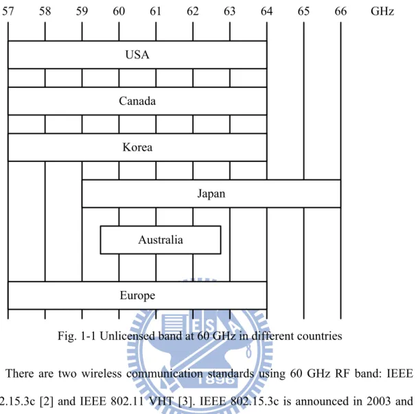
Fig. 1-1 Unlicensed band at 60 GHz in different countries ...2
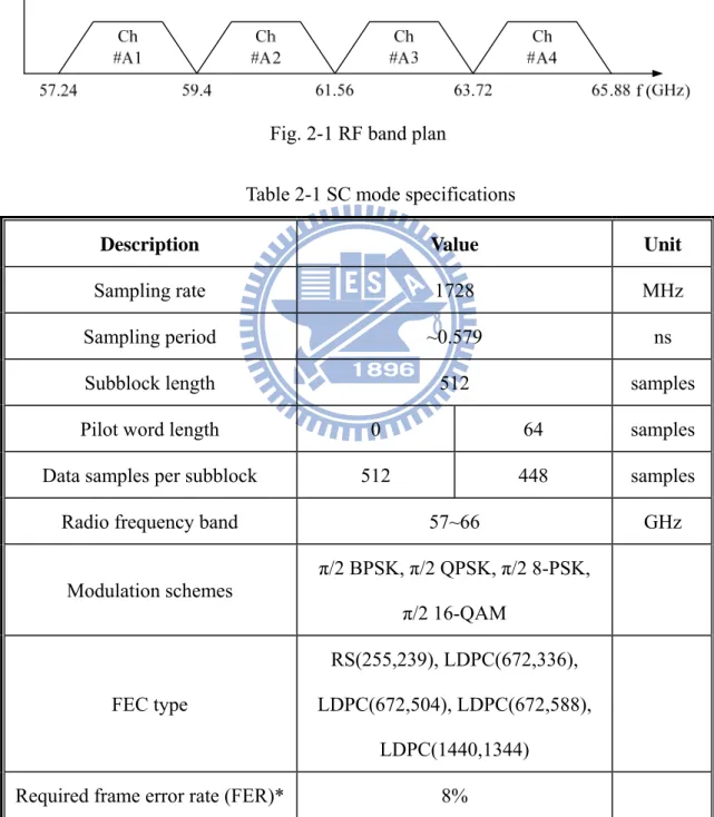
Fig. 2-1 RF band plan ...7
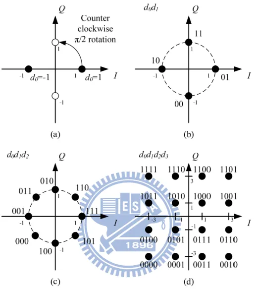
Fig. 2-2 Constellation maps: (a) π/2 BPSK, (b) π/2 QPSK, (c) π/2 8-PSK, (d) π/2 16-QAM...9
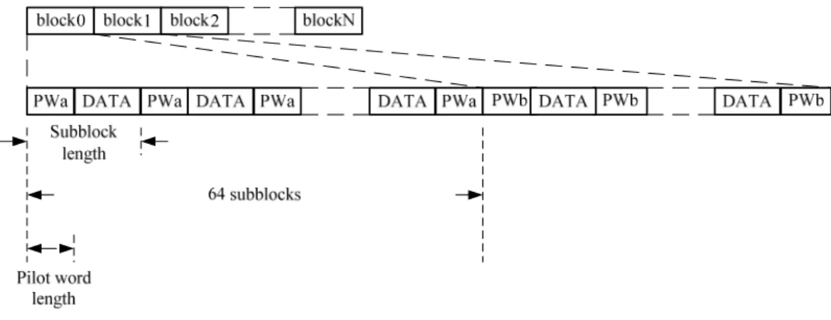
Fig. 2-3 Frame format of block transmission...10
Fig. 2-4 CMS frame format and preamble structure...12
Fig. 2-5 PHY preamble structure ...13
Fig. 2-6 Channel impulse response...16
Fig. 2-7 Channel frequency response...16
Fig. 2-8 Block diagram of receiver ...17
Fig. 2-9 FIR filter structure...18
Fig. 2-10 FIR filter coefficients for TDE...19
Fig. 2-11 Structure of fully parallel FDE ...20
Fig. 2-12 Structure of fully serial FDE ...20
Fig. 3-1 Block diagram of the proposed FDE...24
Fig. 3-2 Noise enhancement ...25
Fig. 3-3 Illustration of adaptive FDE...28
Fig. 3-4 Comparison of training result between LS and LMS...32
Fig. 3-5 Learning curves ...32
Fig. 3-6 Digital modulation...33
Fig. 3-7 Block diagram of π/2 M-PSK mapper...34
Fig. 3-8 The translation at: (a) even sampling time, (b) odd sampling time...34
Fig. 3-9 Block diagram of π/2 M-PSK Demapper and feedback loop...35
Fig. 3-11 Detailed block diagram of the proposed adaptive FDE ...37
Fig. 3-12 Eb/N0 vs. Bit Error Rate ...37
Fig. 4-1 Revised block diagram of the proposed FDE...39
Fig. 4-2 Table of inversed scalar...41
Fig. 4-3 Reduced mapping...42
Fig. 4-4 Structure of the scalar...43
Fig. 4-5 Reduced table ...43
Fig. 4-6 Block diagram of modified divider ...44
Fig. 4-7 Execution order of stages ...45
Fig. 4-8 Block diagram of (a) the proposed FDE, (b) complex multiplier, and (c) complex multiplier with one conjugated input ...49
Chapter 1
Introduction
1.1 60 GHz Radio Frequency Band Wireless Communication
System
The wireless communication technology has been developed for many years. From the telegraph to the WLAN, each system occupies a certain frequency band. When more and more wireless communication systems are developed, the frequency band is much crowded than ever before. Furthermore, when the data rate is increasing, the occupied bandwidth becomes wider. For a newly developed wireless communication system, the selection of the operating frequency band is an important issue.
Because of the improvement on CMOS process, it is possible to design the analog circuit at over GHz sampling rate. Hence, the usage of 60 GHz radio frequency (RF) band becomes possible. Since the 60 GHz RF band is unlicensed in many countries as shown in Fig. 1-1 [1], the development of a wireless communication system on 60 GHz RF band does not need license and becomes a promising technology in recent years. With such wide bandwidth, the data rate can be increased. Moreover, due to the property of short transmission range, the security issue is protected and the reuse rate is very high. Based on these benefits, the wireless communication system using 60 GHz RF band is suitable for indoor and GHz data rate transmission.
57 58 59 60 61 62 63 64 65 66 GHz USA Canada Korea Japan Australia Europe
Fig. 1-1 Unlicensed band at 60 GHz in different countries
There are two wireless communication standards using 60 GHz RF band: IEEE 802.15.3c [2] and IEEE 802.11 VHT [3]. IEEE 802.15.3c is announced in 2003 and the version of the draft at 2009 is No. 8. This standard has three different modes: SC, HSI, and AV mode. SC mode adopts single carrier transmission and the data rate can be up to 5 Gbps. HSI and AV mode are OFDM transmission and the data rate can be up to 4.5 Gbps and 3.8 Gbps respectively. All of the modes operate at 60 GHz RF band. IEEE 802.11 VHT is announced in 2007 and “VHT” stands for “Very High Throughput”. IEEE 802.11 VHT standard uses both 60 GHz and below 6 GHz RF band. The 60 GHz mode is compatible with IEEE 802.15.3c AV mode and that below 6 GHz mode is compatible with IEEE 802.11 series. Both standards focus on indoor, over Gbps data rate wireless transmission.
1.2 Feature of IEEE 802.15.3c
Under the 60 GHz RF band, there are some special properties that influence the channel. Due to strong directivity, wave reflexes, diffracts, and scatters slightly, and the energy of the wave centralizes in a certain angles (about 30°). Since the oxygen absorbs the wave in this RF band, the transmission distance is very short, less than 10 meters, which leads to negligible multipath effect. Based on these properties, IEEE 802.15.3c standard is pronounced for the indoor, over Gbps data rate wireless transmission using 60 GHz RF band. In general, with such a high data rate, we expect the channel would be line-of-sight (LOS), large root-mean-square (RMS) delay spread, slight Doppler Effect, and negligible multipath effect when the wireless communication system operates under the 60 GHz RF band. Using 1728MHz and 2592MHz sampling rate, this system can achieve maximum data rate of 5 Gbps in SC mode and 4.5 Gbps in HSI mode with several modulation schemes (π/2 BPSK, π/2 QPSK, π/2 8-PSK, π/2 16-QAM, 64-QAM).
1.3 Motivation
OFDM has been developed for many years due to its inter-symbol interference (ISI)-free property. With Fast Fourier Transform (FFT) block in the receiver, OFDM turns a group of samples with ISI in the time domain into the ISI-free subchannels, which can be easily equalized by a single-tap equalizer. To eliminate inter-symbol-interference (ISI), a cyclic prefix (CP) of length no less than the channel impulse response (CIR) is inserted in each of the transmitted OFDM symbol and discarded at the receiver. Furthermore, the CP can transform the linear convolution into the circular convolution, which ensures the channel matrix to be a diagonal
matrix. With the insertion of the pilot subcarriers both in time and frequency domain, the equalizer coefficients are updated on the corresponding subcarriers. Then, the rest of the equalizer coefficients can be estimated by doing the interpolation between the pilot subcarriers. Hence, the equalizer coefficients are easily evaluated, and this method is so called channel estimation.
Although OFDM is able to eliminate the ISI, it has the drawback of high peak-to-average power ratio (PAPR). An OFDM signal is composed of N sinusoidal waves, where N is number of subchannels. As N increased, the PAPR gets higher, and the system requires a power amplifier with large linear region in RF end. Furthermore, OFDM suffers from inter-carrier-interference (ICI) caused by carrier frequency offset (CFO) or Doppler Effect, which ruins the orthogonality between each subchannel.
On the other hand, SC is less affected by PAPR and ICI than OFDM while using time-domain equalization. However, the ISI impacts the performance and the computational complexity of time-domain equalizer (TDE) is very high as the RMS delay spread of channel increasing. Research shows that when the CIR increases to certain length, the frequency-domain equalizer (FDE) has less computational complexity than the TDE [4]. With the aid of the cyclic prefix (CP), the FDE can be implemented easily than ever before [5], [6]. Also, single carrier block transmission (SCBT) is formed when the CP divides the continuous data stream into data blocks, like the symbols in OFDM. The number of subchannels is determined by the number of samples in one data block, which is 512 in IEEE 802.15.3c standard. Each of the subchannels occupies 3.375MHz (1728MHz/512 subchannels) bandwidth. Therefore, the SCBT with the FDE is free from ISI and only slightly affected by PAPR [7] and ICI. Moreover, the FDE can be compatible with IEEE 802.15.3c HSI (OFDM) mode
However, there are two major concerns in SCBT with FDE. First, unlike OFDM, there is no pilot subcarrier in SCBT so that the channel estimation method can not be used in the FDE. Under the influence of Doppler Effect, doing equalization without updating the equalizer coefficients is unpractical. Without the aids of pilots, other adaptive algorithm must be used in the FDE. Second, operating at the high sampling rate, the adaptive algorithm should keep the computational complexity as low as possible while the convergence speed will not decrease unsustainably to unconverge [8]. However, the adaptive algorithm with superior convergence properties always comes with high computational complexity [9], [10], which grows nonlinearly. Hence, using channel estimation with training sequence to aid the adaptive algorithm is a suitable way to accelerate the convergence speed without increasing too much complexity. Therefore, the adaptive FDE with the channel estimation can balance the computational complexity and the convergence speed [11].
We propose the FDE using LMS adaptive algorithm with the aid of the channel estimation based on LS method to maintain both advantages from TDE and OFDM with reasonable convergence speed and performance. Also, the hardware sharing and reduction schemes are adopted to ease the computational complexity in the RTL design.
1.4 Thesis Organization
The thesis is organized as follows. In Chapter 2, we explain the SCBT system and give the overview of IEEE 802.15.3c standard. Chapter 3 deals with the detailed mathematical explanation of the proposed FDE. The corresponding hardware design with some low-power architecture techniques and simulation results are presented in Chapter 4. Finally, Chapter 5 is the conclusion and the future work.
Chapter 2
Overview of IEEE 802.15.3c Standard
2.1 IEEE 802.15.3c Specifications
IEEE 802.15.3c is a wireless communication standard based on both SC and OFDM transmission. It uses Common Mode Signaling (CMS) and a preamble attached in front of the data stream. The CMS is specified to enable interoperability among different PHY modes. After the CMS, the frame payload is transmitted in different PHY modes. The preamble is added to aid receiver algorithms related to AGC setting, antenna diversity selection, timing acquisition, frequency offset estimation, frame synchronization, and channel estimation. With insertion of CP, it can reduce the impact of ISI. With channel coding, the system can correct the transmission errors. Furthermore, the standard defines interleaving, scrambler, unequal channel coding, and several modulation scheme to achieve better performance.
2.1.1 Basic Specifications
In this standard, there are three transmission modes: Single Carrier (SC) mode, High Speed Interface (HSI) mode, and Audio/Visual (AV) mode. HSI and AV mode use OFDM transmission, and SC mode is single carrier transmission. Some parameters are listed in Table 2-1 for only SC mode.
shown in Fig. 2-1. The standard indicates that the RF band is divided into four sub-bands such that the Nyquist bandwidth of each sub-band is exactly 1728MHz. In addition, each of sub-bands has 432 MHz spacing to prevent the interference from each other. In this case, the RF band can support 4 transmission bands without any interference.
Fig. 2-1 RF band plan
Table 2-1 SC mode specifications
Description Value Unit
Sampling rate 1728 MHz
Sampling period ~0.579 ns
Subblock length 512 samples
Pilot word length 0 64 samples Data samples per subblock 512 448 samples
Radio frequency band 57~66 GHz
Modulation schemes π/2 BPSK, π/2 QPSK, π/2 8-PSK, π/2 16-QAM FEC type RS(255,239), LDPC(672,336), LDPC(672,504), LDPC(672,588), LDPC(1440,1344) Required frame error rate (FER)* 8%
*: FER is determined at the PHY Service Access Point interface after any error correction methods. The measurement shall be performed in AWGN channel with a frame payload length of 2048 octets.
The standard supports two types of pilot word length: 0 or 64. Transmission with pilot words decreases the data rate, but there are benefits. The pilot word is designated for timing tracking, compensation for clock drift, and compensation for frequency offset error. With these additional supports, the receiver can achieve better performance in long term. The pilot word can also act as the guard interval and the cyclic prefix, which are very useful for the frequency domain equalization. On the other hand, transmission without any pilot word can make the data rate higher but comes with concern of performance loss. It’s a trade-off between the data rate and the performance.
The data is modulated by π/2 BPSK, π/2 QPSK, π/2 8-PSK, or π/2 16-QAM before transmitting in SC mode. The π/2 BPSK is a binary modulation with π/2 phase shift counter clockwise. The mathematical description is:
*
n
n n
z = j d (2.1)
, where dn indicate the data samples and zn are the constellation points.
As shown in Fig. 2-2(a), the π/2 BPSK is equivalent to MSK, which is the continuous phase modulation. The main purpose of the continuous phase modulation is to eliminate the discontinuity between the waveforms. The discontinuity will result in high frequency components in the waveform such that the transmitter requires a power amplifier with larger linear region. There are many applications using this special property of π/2 BPSK, such as symbol timing tracking [12] and differential receiver [13]. The π/2 QPSK, π/2 8-PSK, and π/2 16-QAM are also doing the π/2 phase shift after the mapping with gray encoding. The reason of the π/2 phase shift is to obtain a simple implementation aligning with the π/2 BPSK. The constellation
diagram is shown in Fig. 2-2(b) (c) (d).
Fig. 2-2 Constellation maps: (a) π/2 BPSK, (b) π/2 QPSK, (c) π/2 8-PSK, (d) π/2 16-QAM
2.1.2 Concept of Single Carrier Block Transmission
The standard indicates that the pilot words should be inserted into the data stream every 448 data samples, so the data stream is divided into several small subblocks, which lead to the block transmission, as shown in Fig. 2-3. These pilot words are used for timing tracking, compensation for clock drift, and compensation for frequency offset error. Furthermore, the pilot words act as the cyclic prefix and enable the
frequency-domain equalization.
Fig. 2-3 Frame format of block transmission
The inter-block-interference (IBI) and ICI affect the received signal of SCBT due to the channel distortion. Inserting the guard interval which length is longer than the length of the channel impulse response can eliminate the IBI since the previous subblock can not interfere the incoming subblock. In order to prevent the ICI while using the FDE, the guard intervals in the front and the back of the subblock should be the same, and this is so called the cyclic prefix. The CP can maintain each subchannel to be orthogonal and reduce the effect of ICI. Besides, the CP translates the linear convolution into the circular convolution, which results in a simple diagonal channel matrix in frequency domain. As the result, evaluating the filter coefficients is much easier than in time domain. We will explain the fact in the following paragraphs.
The received subblock rn and its frequency domain form Rk is described as follows,
where dn is transmitted signal and h is CIR with length L and are extended to length N
1 1 2 0 0 { } { } ( ) k n n n N N j k N m n m n m R FFT r FFT d h h d e π − − − − = = = = ⊗ =
∑ ∑
⋅ (2.2)Since dn is cyclic prefixed and periodic, the equation can be written as:
1 1 2 0 0 1 1 2 0 0 1 1 1 1 2 2 0 0 0 0 1 2 2 0 ( ( )) ( ( )) 1 ( ( )) 1 ( ) ( n N N j k N k m n m pN n m p n N N j k N m t n m t pN n m t p n m t n N N N N j k j k N N m t n m t k m N t j k j k N N m t m t R h d e h d e h d e e N h e d e N π π π π π π δ − − ∞ − − − = = =−∞ − − ∞ ∞ − − − − = = =−∞ =−∞ − − − − − − − = = = = − − − = = = ⋅ ⋅ = ⋅ ⋅ ⋅ = ⋅ ⋅ ⋅ = ⋅ ⋅ ⋅
∑ ∑
∑
∑ ∑ ∑
∑
∑ ∑ ∑
∑
∑
1 1 0 0 ) N N n k k H D − − = = ⋅∑ ∑
(2.3)Because of the circular convolution, we can easily recover the transmitted data and evaluate the filter coefficients:
ˆ { } ˆk n k k k k R d IFFT H D W R = = (2.4)
2.1.3 Equalization Related Specifications
In this standard, there are some well known data streams that are assigned to different specific purposes, i.e. MAC layer control signal, the piconet coordinate signal, or the performance improving signal. This section will introduce the specific signaling directly related to the equalization.
The CMS is a low data rate SC mode and specified to enable the switching among different PHY modes. It’s also used for transmission of the beacon frame, sync frame, command frame, and training frame in the beamforming procedure. The forward error correction (RS(255,239)) and code spreading (spreading factor: 64) are used to ensure the correctness of the CMS. A PHY preamble is added to aid the receiver algorithms such as AGC setting, timing acquisition, frame synchronization, and channel estimation.
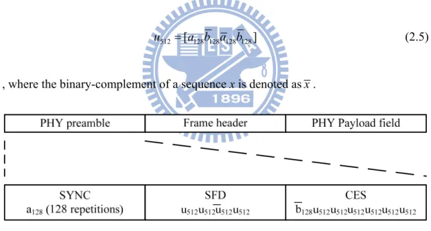
As shown in Fig. 2-4, the preamble is prior to the frame header and PHY Payload field. It consists of the Golay complimentary sequences a128 and b128 of length 128,
listed in Table 2-2. The code u512 is constructed as below:
512 [ 128 128 128 128]
u = a b a b (2.5)
, where the binary-complement of a sequence x is denoted asx .
Fig. 2-4 CMS frame format and preamble structure Table 2-2 Golay sequences
Sequence name Sequence value
a128 C059950CC0596AF33FA66AF3C0596AF3
b128 30A965FC30A99A03CF569A0330A99A03
The main purpose of SFD field is to validate the beginning of a frame. The CES field is assigned to do channel estimation.
As mentioned in Section 2.1.2, the SCBT is suitable for frequency domain equalization due to the CP. Although there is no periodic stream in u512, it becomes
cyclic prefixed withb in previous u128 512. Combined with the leadingb , the first u128 512
is also cyclic prefixed. As the result, there are 6 subblocks available in the CES field to do channel estimation.
PHY preamble
After the CMS, the system will switch to the designated mode and begin to transmit the data payload. In each beginning of transmission, the transmitter will send a PHY preamble to aid the receiver algorithms, just like the one in CMS. In SC mode, the preamble is transmitted at the rate of 1728 MHz. The PHY preamble structure is shown in Fig. 2-5.
Fig. 2-5 PHY preamble structure
Like CMS preamble structure, the PHY preamble consists of SYNC, SFD, and CES field. Each of the field functions like the one in CMS preamble: SYNC field for frame detection, SFD field for validating the beginning of the frame, and CES field for channel estimation. The Golay sequenceb and128 u ensures the cyclic prefix 512
property and is also useful information for frequency domain equalization. Pilot Channel Estimation Sequence(PCES)
The PCES insertion is an optional feature that allows the system to re-acquire the channel information periodically. To add the PCES, the data stream is divided into data blocks with each data blocks has 64 subblocks, as shown in Fig. 2-3. Each data block is followed by a PCES. The PCES is the Golay sequence a128 followed by the
CES field in the PHY preamble mentioned above and is shown in (2.6). Since PCES contains the information of the CES field, this cyclic prefixed signal can provide the channel information periodically.
128 128 128 128 128 128
[ ]
PCES= a b a b a b (2.6)
2.2 Channel Model
IEEE 802.15.3c standard is for an indoor, over GHz data rate, wireless communication system using 60 GHz RF band. In 60 GHz RF band environment, the channel model has some special properties that are much different from those below 10GHz RF band channel. These properties are listed below:
High Path Loss
While the EM wave passes through the medium, the medium absorbs the energy and limits the distance that the EM wave can travel. The more energy it lost, the shorter it can travel. The ratio of energy loss is mainly depends on the characteristic of the medium and the EM wavelength. The wavelength of 60 GHz wave is close to the length of the oxygen chemical bond, so the wireless communication in 60 GHz RF
band suffers the tremendously high path loss. As the result, the transmission distance is limited to about 10 m in maximum. Moreover, the effect of the multi-path fading is reduced since the non-line-of-sight (NLOS) wave travels more distance and loses more energy than the line-of-sight (LOS) wave.
Strong Directivity
The strong directivity means that the EM wave energy almost centralizes in the small angle. From the formula of the diffraction:
2 0 sin ( ) sinc (d ) I θ I θ λ = (2.7)
,where I is the intensity profile and basically is a sinc function related to the diffraction angle θ and the wavelength λ. For a small λ, the intensity drops rapidly while θ increasing. This phenomenon shows that the antenna can only transmits or receives the signal in the small angle. In conclusion, the NLOS path has lower path gain relative to the LOS path, and the multi-path fading effect is once more reduced.
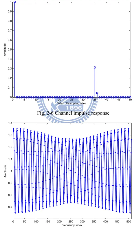
The channel model is based on the golden set released by IEEE 802.15.3c group [14]. The golden set, shown in Fig. 2-6, 2-7, provides a set of the static channel models in 60 GHz RF band and the one with the largest RMS delay spread is chosen as the worst case channel model, which is 12.73 ns. To simulate the time-variant effect, the Jakes model is used as the Doppler Effect. Considering the human moving speed in indoor environment, the relative velocity is assumed to be 4.5 km/h, which is 250 Hz frequency shift according to (2.8):
0
v f f
c
,where v is for relative velocity between the receiver and the transmitter, c for velocity of EM wave, and f0 for the frequency of the carrier. The negative sign means the
receiver is moving toward to the transmitter. The frequency shift is 7.41*10-3% of the subcarrier spacing (3.375MHz). 0 5 10 15 20 25 30 35 40 45 50 0 0.1 0.2 0.3 0.4 0.5 0.6 0.7 0.8 0.9 1
Delay (1/sampling rate)
A
m
plit
ud
e
Fig. 2-6 Channel impulse response
0 50 100 150 200 250 300 350 400 450 500 0.7 0.8 0.9 1 1.1 1.2 1.3 1.4 Frequency index A m plit ud e
2.3 Comparison of Time and Frequency Domain Equalizer
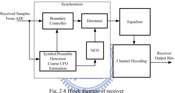
The main functional blocks of the baseband receiver are shown in Fig. 2-8. After the signal is sampled by ADC, we use synchronizer to detect the boundary of the frame. Then, the data is equalized to eliminate the channel effect and sent to channel decoding. The purpose of channel decoding is to correct the error bits using the algorithm of channel coding.
Symbol/Preamble Detection Coarse CFO Estimation Boundary Controller Derotator NCO Received Samples From ADC Receiver Output Bits Equalizer Channel Decoding Synchronizer
Fig. 2-8 Block diagram of receiver
We have overviewed the channel model in both time and frequency domain in Section 2.2. In this section, the discussion focuses on the comparison of time and frequency domain equalizer in terms of the computational and hardware complexity base on the channel model.
Time Domain Equalizer(TDE)
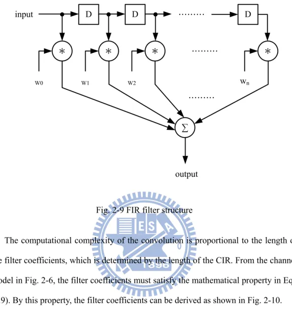
The basic structure of the TDE is the FIR filter, which performs the convolution between data stream and the filter coefficients. A simple illustration of the FIR filter is shown in Fig. 2-9.
……… D D ……… D * * * ∑ ……… input * W0 W1 W2 wn output
Fig. 2-9 FIR filter structure
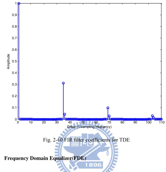
The computational complexity of the convolution is proportional to the length of the filter coefficients, which is determined by the length of the CIR. From the channel model in Fig. 2-6, the filter coefficients must satisfy the mathematical property in Eqn. (2.9). By this property, the filter coefficients can be derived as shown in Fig. 2-10.
[
]
* 1 0 0 0
h w= (2.9)
From Fig. 2-10, the required number of the filter coefficients is 104, which is much longer than the wired communication system [15]. If the structure illustrated in Fig. 2-9 is used, then the number of the required complex multiplications is also 104. Therefore, the operation time for the 104 complex multiplications is one sampling period. It’s almost impossible to implement the hardware with GHz sampling rate indicated by the standard. Although the parallel design can increase the throughput of TDE, the complexity grows linearly with the number of coefficients.
0 10 20 30 40 50 60 70 80 90 100 110 0 0.1 0.2 0.3 0.4 0.5 0.6 0.7 0.8 0.9 1
Delay (1/sampling frequency)
A
m
pl
itude
Fig. 2-10 FIR filter coefficients for TDE Frequency Domain Equalizer(FDE)
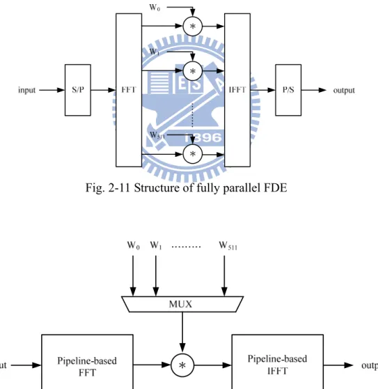
A simple illustration of fully parallel FDE is shown in Fig. 2-11. The input passes through Serial-to-Parallel block and transforms to frequency domain by FFT. Then, the frequency domain data is multiplied with coefficients W and then transformed back to time domain by IFFT. Unlike TDE, the number of coefficients in FDE is fixed no matter how the length of the channel impulse response changes. The potential problem is when the length of the CIR is longer than the length of the CP. In that case, the circular convolution is ruined and FDE fails to equalize the channel effect. However, the channel model shows that the maximum length of CIR is far less than the length of CP, so we do not consider the problem in the thesis.
The advantage of FDE is lower computational complexity than TDE when the length of CIR is long enough. Assuming that the computational complexity of
FFT/IFFT is NlogN, the total computational complexity of FDE is 2NlogN+N, where N is 512 based on the standard. Therefore, the average computation on one sample is 2logN+1, which is 19. Moreover, the equalization can be reduced using the pipeline-based FFT/IFFT as shown in Fig. 2-12. This pipeline-based design can be parallelized easily by adding multipliers of the equalization. Thus, it can be used in high sampling rate communication system without too much overhead. After some modifications, the FDE can also support OFDM mode, and the overhead of FFT is reduced.
Fig. 2-11 Structure of fully parallel FDE
Fig. 2-12 Structure of fully serial FDE
problem of large computational complexity in the hardware design. On the other hand, FDE is suitable for high sample rate since it’s easy to do parallelism. The drawback is that additional CP reduces the data rate. The comparison is listed in Table 2-3.
Table 2-3 Comparison between TDE and FDE
TDE FDE Coefficient number Proportional to the length of
CIR (104) Subcarrier number (512)
Complexity High (104 multiplications
on one sample)
Low (19 multiplications on one sample)
Data throughput High
(sampling rate*1)
Low
(sampling rate*448/512)
Storage requirement 104 coefficients 512 coefficients Compatible with
OFDM
No Yes
2.4 System Requirements and Design Considerations
The IEEE 802.15.3c standard indicates the system requirements mentioned in Section 2.1.1. One of the requirements is the 1728 MHz sampling rate. The sampling rate equals to the throughput of the system. The throughput is increased with the improvements of CMOS process and architecture, but over GHz throughput is still a challenge for hardware design. Moreover, high throughput also means that high power consumption in the digital circuit. Also, the choice of the architecture determines the power consumption. Hence, there two design considerations on high sampling rate: architecture and power consumption.
The pipelined structure and parallel structure are commonly used for high throughput design. The pipelined structure can increase the clock rate by inserting the registers into the combinational circuit. However, the dynamic power is also increased
with clock rate. On the other hand, parallel structure increases the throughput by copying the structure without increasing the clock rate, but the area and static power grows with the number of copies. Hence, our considerations on architecture and power consumption mainly focus on how many copies we want and how fast the clock rate is.
Another system requirement is the bit error rate (BER). According to the FER and frame size, the required BER is 1.54*10-4. Hence, the design consideration is the performance and the cost of computational complexity. First of all, we consider the algorithm that can be realized in hardware design. Since the throughput is very high, we should keep the complexity as low as possible. Then, we should consider the channel model. The channel model in Section 2.2 contains Doppler Effect, so it is time-variant. Thus, the algorithm of the equalizer must have the ability to update its coefficients with time. Third, the length of the training sequence is determined by the standard as mentioned in Section 2.1.3, so the algorithm should be ready within the training stage. Hence, we have to choose the reasonable computational complexity algorithm which satisfies the BER requirement.
Chapter 3
Fast Convergent Adaptive Frequency
Domain Equalizer
3.1 Review of Frequency Domain Equalization
In Section 2.1.2, we derive the formula of circular convolution, which can be transformed into a simple multiplication in the frequency domain:
R H D= ⋅ (3.1) ,where H is a diagonal matrix. To recover the transmitted data, we multiply the inverse of H on both sides of equation:
1 1
H− ⋅ =R H− ⋅ ⋅ = H D D (3.2) , where the inverse of H is also a diagonal matrix. After IFFT and CP removal, we can fully recover the transmitted signal dn.
The above equations describe the ideal case: no AWGN and time-invariant channel. In reality, the white noise always exists due to the thermal noise, and the channel varies with time due to many effects, such as related movement, air flow, or moving object. Thus, the equation should be:
( )
k k k k k
the subchannels. If we simply multiply the inverse of Hk all over the time, the
time-variant effect will corrupt the data. Furthermore, to get the accurate inverse of Hk
is a difficult job under AWGN. To break through the predicament, the first thing is to overcome AWGN and get the inverse of Hk as accurate as possible. Then, an adaptive
algorithm is performed to track the changes in the time-variant channel. In this way, the time-variant component Jk(t) is no more a trouble in the equalization. Based on the
idea, the block diagram of the proposed adaptive FDE with channel estimation is shown in Fig. 3-1. The LS channel estimation evaluates the initial value of coefficients by using the CMS and the preamble as the training sequence. Then, the data payload is transmitted and equalized by FDE. The LMS adaptive algorithm updates the coefficients against the time-variant channel.
Fig. 3-1 Block diagram of the proposed FDE
3.2 Channel Estimation
In the beginning of the transmission, the transmitter sends the training sequence u512 located in CES field of CMS to assist the equalization as shown in Fig. 2-4. With
the training sequence, we can easily estimate the channel matrix Hk, which is the
512, k k k R H U = (3.4)
This solution is known as zero-forcing (ZF) method. The benefit is the simple implementation, but this method suffers from a problem: noise enhancement. With AWGN, the Eqn. (3.4) is revised as Eqn. (3.5).
k k k k k U W H U N = ⋅ + (3.5)
The noise enhancement occurs when the channel gain Hk is so small that the noise
Nk is the dominant part in received signal. In that case, especially with large Nk, the
estimation result is far away from perfect estimation as illustrated in Fig. 3-2.
410 420 430 440 450 460 0 1 2 3 4 5 6 7 8 9 10 Subchannel index A m pl itude Perfect Estimation Least-Square Zero-Forcing
Fig. 3-2 Noise enhancement
than using ZF. The main point of LS is to minimize the sum of the squares of the error. First of all, the equalization can be described as:
512,k k k U R W = (3.6)
Second, apply the error caused by AWGN, where i stands for i-th U512 in CMS.
512, , , 512, , , k i k i i k k i i k i k U R W U R W ε ε = + = − (3.7)
Then, we need to minimize the sum of the squares, so let the partial derivative on Wk be zero. 512, , 2 2 , 2 512, , 512, , , 2 3 ( ) (2 2 ) 0 k i i k i i i k k i k i k i i k k k U S R W U U S R W W W ε = = − ∂ = − = ∂
∑
∑
∑
(3.8)Finally, the solution of Wk indicates the minimum of S.
2 512, , , 512, , ( ) k i i k k i k i i U W R U =
∑
∑
(3.9)Since U512 is constant all the time, it can be rewritten as:
2 512, 512, , 512, , 6 1 ( ) 6 k k k k i k k i i i U U W R U R = =
∑
∑
(3.10)512, , 512, 1 ( ) 6 k k k i k k i U W H U N = +
∑
(3.11)With the summation of Nk, the noise enhancement is reduced since the mean of
AWGN is zero. We can obviously observe the benefit from Fig. 3-2. The numerical analysis in Table 3-1 also supports the result.
Table 3-1 Numerical analysis between LS and ZF
Method Mean of error Variance of error
LS 0.0176 + 0.0197i 1.4251 ZF 0.6073 + 1.6084i 5.7079
3.3 Adaptive Equalization
In OFDM system, the pilot subcarriers are needed to track the changes of the time-variant channel. However, we can not insert any known message in the frequency domain since the whole system is SCBT. Thus, our FDE requires an adaptive algorithm against the time-variant channel.
3.3.1 Adaptive Algorithm
There are many adaptive algorithms developed in the literals. The issues of these algorithms mainly focus on their computational complexity and convergence speed. The widely used algorithms are Minimum-Mean-Square-Error (MMSE), Recursive-Least-Square (RLS), and Least-Mean-Square (LMS) [16], [17], and there are many improvements on these algorithms. Due to 1728MHz sampling rate, high computational complexity algorithm is not suitable for such high sampling rate
design. Based on the considerations, we will prove that LMS is a good choice for the FDE.
Let’s consider the block diagram of the adaptive FDE shown in Fig. 3-3. R is the input from FFT, and the adaptive FDE do the equalization and update filter coefficients W. The FDE output is sent back to time domain and made decision by the demapper. The error E is the difference between FDE output and the training sequence (or sliced output when the data is transmitted).
Fig. 3-3 Illustration of adaptive FDE
The idea of LMS algorithm is to use the method of the steepest descent to find a set of W which minimizes the cost function. In our design, the FDE takes a subblock into the equalization, so the cost function should involve a block of errors, which is so called Block LMS (BLMS) [18]. However, since the equalization is independent of each subchannel, we can consider each cost function Ck in each subchannel
independently instead of whole subblock.
2
{ }
k k
C =Ex E (3.12)
The notation of Ex{.} rather than E{.} is used to denote the expect value because we don’t want to be confused with the error E. Then, applying the steepest descent is
to take the partial derivative with respect to the filter coefficients W.
* *
{ } 2 { } C Ex EE Ex EE
∇ = ∇ = ∇ (3.13)
Since the equalization is independent of each subchannel, Eqn. (3.13) is equal to zeros when the error E and coefficient W are in different subchannel. Then, substituting E with received signal R, we can rewrite Eqn. (3.13) as
* ( ) 2 { } k k k k k k k k k k k dE d D W R R dW dW dC Ex R E dW − = = − ∴ = − ∵ (3.14)
, where k is the subchannel index. Now, these derivatives point towards the steepest ascent of the cost function. To find out the minimum of the cost function, we take a step size of
2
μ
in the opposite direction of the derivatives.
, * , 1 , , , { } 2 k n k n k n k n k k k n dC W W W Ex R E dW μ μ + = − = + (3.15)
, where n indicates the subblock index.
For simplification, the expected value can be reduced, and the whole LMS algorithm can be simplified as:
LMS: *
, 1 ,
k n k n k k
W + =W +μR E (3.16)
The derivations of MMSE and RLS can be found in [16], [17]:
MMSE: * 2 * 2 k k n k k s H W H H σ σ = + (3.17)
RLS: * 1 1 n n n n n Y WR U PY g U YU W W g E λ + = = = + = + (3.18) , where 2 n σ and 2 s
σ are variance of noise and signal respectively, Y is equalized signal, U is the intermediate vector, and gn is the gain vector.
Compared with MMSE [19]-[21] and RLS [22], [23], the LMS algorithm has less computational complexity than RLS since there is only one multiplication for updating on one subchannel. In hardware design, more operations on updating will cause the longer feedback latency. The latency will impact the performance since the equalizer can not update immediately. It is more sensitive to the latency especially in high sampling rate and deep pipelined system since the latency is much longer. Furthermore, the low computational complexity leads to low power consumption. The low power issue is more important in the modern SOC design. In that case, LMS also has the advantage of low power consumption property. On the other hand, MMSE has less computational complexity than RLS, but it requires the information of SNR, which is hard to be evaluated since there are Doppler and channel Effect on the received signal. Although there are some algorithms trying to do SNR evaluation, the result is still not reliable in the practical system. Based on these considerations, LMS is suitable for FDE in high sampling rate design and can also achieve the required BER with LS channel estimation mentioned in Section 3.3.2.
3.3.2 Convergence Speed Acceleration
increasing the step size [24]. However, compared with other algorithms, LMS still suffers the slow convergence speed [25] problem. Hence, the training time of LMS takes longer than others, and it requires longer training sequence to do training. According to the standard, the training sequence is available in CES filed of CMS preamble and PHY preamble. However, there are only 6 U512 for training before CMS
payload, so the training result of LMS is not good enough as compared with LS channel estimation.
From the analysis result shown in Fig. 3-4 and Table 3-2, LS channel estimation has a better performance in the view of mean and variance of the error after the training stage. Moreover, the channel model is almost the best case for LMS since the perfect estimation result is so close to the initial value for LMS training procedure, which is an all-pass filter with uniform filter gain. The learning curve is shown in Fig. 3-5. The simulation is under the channel model and 10dB AWGN. LMS only algorithm takes about 35 subblocks to achieve the same performance of LS-LMS combined algorithm. The MSE of first six subblocks is zero since LS is doing the average on these six points. The result supports that the convergence speed of the combined algorithm is indeed faster than single LMS algorithm.
Compared with adaptive TDE, the adaptive algorithm has an initial value of the coefficients with the aid of the channel estimation in the frequency domain. Hence, we can choose a low computational complexity algorithm with slower convergence speed. By doing so, we can balance the tradeoff of performance and hardware complexity.
Table 3-2 Numerical analysis of training result between LS and LMS
Method Mean of error Variance of error
LS 0.0213 + 0.0124i 0.0605 LMS -0.2533 + 0.1042i 0.0896 330 340 350 360 370 380 390 400 410 420 0 0.2 0.4 0.6 0.8 1 1.2 1.4 1.6 Subchannel index A m pl itude Perfect Estimation LS LMS
Fig. 3-4 Comparison of training result between LS and LMS
0 10 20 30 40 50 60 70 101 102 103 104 Subblock MSE LMS LS + LMS
3.4 Demapper
In the transmitter of the digital communication system, the digital modulation transforms the digital bit stream to an analog passband signal. The block diagram is shown in Fig. 3-6. First, the mapper converts every n-bits into one complex symbol according to the constellation map. After the Digital-to-Analog Converter (DAC), the discrete data stream becomes the continuous square wave. The pulse shaper transforms the square wave to band-limited waveform and reduces the frequency bandwidth. Finally, the mixer transforms the baseband signal to the passband signal with the carrier.
Mapper DAC cos(ωct) -sin(ωct) Pulse shaper Baseband digital stream Passband analog signal
Fig. 3-6 Digital modulation
In IEEE 802.15.3c standard, the constellation maps are π/2 BPSK, π/2 QPSK, π/2 8-PSK, and π/2 16-QAM. The π/2 means that the symbol does counterclockwise π/2 phase shift after M-PSK mapping as shown in Fig. 3-7. The purpose of counterclockwise π/2 phase shift is to generate the continuous phase waveform, which results in a constant-modulus signal when using BPSK. The constant-modulus signal can reduce the problem caused by the non-linear distortion since the translations between each symbol never pass through the origin as illustrated in Fig. 3-8.
Fig. 3-7 Block diagram of π/2 M-PSK mapper I Q 1 1 -1 -1 I Q 1 1 -1 -1 (a) (b)
Fig. 3-8 The translation at: (a) even sampling time, (b) odd sampling time After the equalization in the receiver, the demapper converts the complex symbol back to the digital bit stream. For the π/2 M-PSK demapper, the first thing is doing the clockwise π/2 phase shift. Then, the slicer makes the decision on the complex symbol with noise. Finally, the M-PSK demapper converts the complex symbol back to the digital bit stream as shown in Fig. 3-9.
M-PSK constellation demap clockwise π/2 phase shifter π/2 M-PSK demapper From IFFT output To EQ output Feedback to FFT π/2 M-PSK mapper
Fig. 3-9 Block diagram of π/2 M-PSK Demapper and feedback loop
From Section 3.3, we know that the adaptive FDE needs the decision result to perform the algorithm. In this case, the block diagram in Fig. 3-9 can be revised as shown in Fig. 3-10. Since the π/2 phase shift doesn’t change the boundary of the constellation map of π/2 M-PSK, except π/2 BPSK, the slicer can be put before the π/2 phase shifter. For π/2 BPSK, we just do the decision on the real/image axis at even/odd sampling time since the data is modulated in that order. Therefore, we don’t need to do the counterclockwise π/2 phase shift again after slicing and reduce some hardware resources.
3.5 System Architecture and Performance
The proposed FDE operates based on equations in sections of 3.2, 3.3, and 3.4, and the detailed block diagram is shown in Fig. 3-11. In the simulation, the signals are interfered by channel model and AWGN and are assumed to be perfectly synchronized. The system flow is explained as follows:
1. In the beginning, the channel estimation evaluates the filter coefficients with training sequences by LS method.
2. When training sequences is done, the cyclic prefixed data stream is transmitted. The adaptive FDE equalize the received signal.
3. After equalization, the signal is sent to decision circuit, which functions as a slicer.
4. Using the error between equalized and sliced signal, the adaptive FDE updates the filter coefficients by LMS algorithm.
To evaluate the performance, the channel model we use is based on the IEEE 802.15.3c standard group with Jakes’ model, mentioned in Section 2.2. The whole transmitted sequence is composed of CMS, preamble, PW, data, and PCES. The CMS and preamble are used for training and PW works as cyclic prefix. The simulation results are shown in Fig. 3-12. The whole testing environment is built with C language. For each testing point, the length of the transmitted sequence is 448000 samples. Based on the standard, the error rate criterion is set to 1.54*10-4 after any error correcting method. From the figure, our adaptive FDE requires about 10 dB Eb/N0 to achieve this criterion. Comparing to optimal receiver, the loss is only 1.5 dB for both π/2 BPSK and π/2 QPSK.
The fixed-point simulation model is determined by following procedure. First, we quantize the input to minimum word length without significant performance loss. Then, we quantize the next data path. Step by step, we can finally find out the word length of each data path and ensure the performance loss in a reasonable range.
Fig. 3-11 Detailed block diagram of the proposed adaptive FDE
0 1 2 3 4 5 6 7 8 9 10 11 12 10-5 10-4 10-3 10-2 10-1 100 Eb/N0(dB) BE R AWGN pi/2 BPSK pi/2 QPSK pi/2 BPSK (fixed-point) pi/2 QPSK (fixed-point)
Chapter 4
Architecture Design and Hardware
Reduction
4.1 Design Specifications and Architecture
IEEE 802.15.3c standard focuses on over Gbps data rate wireless communication. To achieve the target, there are two key features in the standard. The first one is the usage of the 60 GHz RF band. The unlicensed RF bandwidth is wide enough to support the usage of large bandwidth. The transmission rate is proportional to the bandwidth, so using the unlicensed 60 GHz RF band is essential. The second one is the ultra high sampling rate. Although there are many methods to achieve the target of high data rate, like using higher modulation or multi-input and multi-output (MIMO) system [26], raising the sampling rate is the most direct way since the data rate is proportional to the sampling rate. With the moderate modulation scheme, the data rate could be twice or three times of the sampling rate. In this way, we can easily achieve the target of over Gbps data rate. Based on these features, we propose LS-LMS combined FDE in Chapter 3. The block diagram shown in Fig. 3-11 is redrawn in Fig. 4-1 due to the hardware design considerations. In the following sections, we will discuss our hardware design. However, FFT and IFFT are not the design target in this thesis.
Fig. 4-1 Revised block diagram of the proposed FDE
In modern CMOS process, the issue of power consumption becomes more and more important. There are many methods to reduce the power consumption when we design the hardware, such as using low computational complexity algorithm, substituting high complexity arithmetic unit with lower one, or sharing the hardware resources. By using these methods, we can reduce the chip area and the switching power consumption. Meanwhile, the leakage power is also reduced when the chip area is reduced.
4.2 Divider Free LS Method
In Section 3.2, Eqn. (3.10) indicates LS method needs a complex division. There are two ways to avoid the division. One is using the phase operation as shown in Eqn. (4.1), and the other one is to multiply the conjugate of the divisor both on the denominator and the numerator as shown in Eqn. (4.2).
512, 512, , 2 512, 2 2 512, 2 1 6 k k k k k i i k u k r k u r k U U W R R U R U R θ θ θ θ = = ∠ = ∠ = ∠ −
∑
(4.1) 512, 512, , * 512, * * 512, 2 1 6 k k k k k i i k k k k k k k U U W R R U R R R U R R = = = =∑
(4.2)The phase operation replaces the complex division into one square root function, two square functions, one scalar division, and one subtraction. However, the transformation between the phasor and complex number requires trigonometric function, as shown in Eqn. (4.3). Although there are some realistic designs, the hardware cost is still too high.
512 512, 512, 2 2 2 512 512, 512, 512, 1 512, tan r i r i i u r U U iU U U U U U θ − = + = + = (4.3)
Eqn. (4.2) transforms one complex division to one complex multiplication, one square function and one scalar division. This method is generally used when we calculate the complex division. However, there is one scalar division, which is much more complex than a multiplier [27].
Since the division is an inversed multiplication, then multiplying an inverse of the scalar is a commonly used method. To find out the inverse, we can try to use a table with all possible inverse of the scalar, and we can easily implement it with a ROM as illustrated in Fig. 4-2. The bit width is determined by the accuracy of the inverse, and the word width is determined by the word length of the scalar. According to the simulation result of fixed-point C language, the bit width should be 13 bits and the word width is 14 bits to maintain the performance. Therefore, the size of the ROM is 214*13, which is 213k bits. The cost is reduced, but the ROM still takes large area.
To reduce the size of the ROM, we can try to reduce the bit and word width. Since the accuracy is already determined by bit width, we need to focus on the reduction of the word width. By observing the inverse, we can find out that the inverse is almost the same in nearby words. An example is shown in Eqn. (4.4), the difference between 1/128 and 1/129 is so small that they can not represented in 13 bits. Therefore, nearby scalars can all map to the same inverse stored in the table, as illustrated in Fig. 4-3.
Fig. 4-2 Table of inversed scalar
N is the reference scalar and Δn is the difference. Taking the property of the scalar into consideration, we can see that the scalar is always positive since it’s the result of the square function. Hence, we can reconsider the scalar structure in Fig. 4-4. We can just look up the table according to the significant bits regardless of sign bits and Δn. From the simulation results, the optimal length of the significant bits is 4. The reduced table is shown in Fig. 4-5 and the size is 24*11*13, which is 2288 bits.
10 2 1 0.0078125 128 1 =0.0077519 129 1 -1 =0.0000606 0.0000000000000001 128 129 = = (4.4) 1 1 1 ( ) ( 1) n N N N n N N n N n ε = − = Δ = + Δ + Δ + Δ (4.5) 1/128 Decoder 0.0078125
……
……
=>
map to 1/128=>
access 1/129 1/130 1/131Fig. 4-4 Structure of the scalar Inverse of 1 Inverse of 2 Inverse of 3 Inverse of 15 Inverse of 16,17 Inverse of 18,19
……
Inverse of 30,31 Inverse of 32,33,34,35 Inverse of 36,37,38,39…
Fig. 4-5 Reduced tableSince Δn bits are ignored, they looks like zeros. We can represent them as another form as illustrated in Eqn. (4.6), where SB means the significant bits.
*2 n
scalar SB= Δ (4.6) The meaning of these Δn bits are doing the left shift on SB, so the inverse of the scalar can be represented as Eqn. (4.7).
1 1 2 *2 n n inverse scalar SB SB −Δ Δ = = = (4.7)
The 2-Δn is doing the right shift on the inverse of SB. Since SB has only 4 bits, the table has to store only 16 inversed scalars, which cost 208 bits storage area. Through this procedure, we substitute a division with one small ROM and one multiplier. The block diagram is shown in Fig. 4-6. Compared with a real divider in DesignWare, the modified version has smaller area and can satisfy the requirement of high clock rate operation. Furthermore, the size of the ROM is 99.99% off by the method mentioned above.
SB
Δn
Table
U
512,kR
k*Right
Shifter
LS
result
R
kR
k*Fig. 4-6 Block diagram of modified divider
4.3 Hardware Sharing
4.3.1 Multiplier Sharing
Since we want to maintain balance between the performance and the power consumption, we combine LMS and LS to achieve the target. LMS and LS both have the property of low computation complexity, which means low power consumption. With the aid of LS, we can get a better training result and improve the performance of
LMS. However, using LS needs additional area and power, which is contradictory to our target of low power design. To solve this contradiction, we need to do some methods of reduction.
According to Section 3.5, the system flow enters the training stage first. After the training stage, the transmitter starts to transmit the data stream. It’s obvious that these two stages don’t overlap with each other. In the training stage, only LS related circuits are operating, but LMS and one-tap equalizer related circuits are idle. On the other hand, the LS related circuits are idle in the data transmitting stage as illustrated in Fig. 4-7.
Fig. 4-7 Execution order of stages
According to Fig. 3-11 and Eqn. (4.2), LS channel estimation takes one complex multiplication with one conjugated input, one complex power measurement unit, and one divider, which is substituted with two multipliers. There are total 8 multipliers for the computation of LS in the training stage. On the other hand, the LMS only takes one complex multiplication with one conjugated input as shown in Eqn. (3.16). Then, the one-tap equalizer needs one complex multiplier. The FDE requires also 8 multipliers to operate in the data transmitting stage. Based on these observations, we can list the operation table in each stage as shown in Table 4-1 and figure out how to share the hardware resource.
Table 4-1 Operation requirement of the proposed FDE
Training stage Data transmission stage
LS LMS One-tap EQ
Complex multiplication with one conjugated input
19 bits * 16 bits (4 real multipliers) 10 bits * 7 bits (4 real multipliers) 0 Complex multiplication 0 0 21 bits * 15 bits (4 real multipliers) Complex power measurement unit 13 bits * 13 bits (2 real multipliers) 0 0 Modified divider (scalar multiplier) 11 bits * 13 bits (2 real multipliers) 0 0
Only the size of the complex multiplication with one conjugated input has to be extended to 19 bits * 16 bits, and the complex power measurement unit and the modified divider multipliers are all shared with the one-tap EQ. Hence, the area of the combined circuit is reduced 47% compared with no-sharing circuit. The reduction is tremendously important since these multipliers takes 60% area among the proposed FDE before the sharing.
4.3.2 Register Sharing
We have two storage components in the architecture, which are SISO_1 and SISO_2 in Fig. 3-11. The purpose of the storage blocks is to store the information temperately. SISO_1 is used to store the summation of received signal R, and SISO_2 is to store the filter coefficients. In the hardware design, these blocks are both replaced with the storage device, such as random logic register file or RAM. Since the filter coefficients are fetched by both LMS and one-tap EQ, we prefer the register file rather than RAM. Furthermore, the two storage blocks can share the same register file since they operate in different time slot. From the synthesis result, the area of the
register file is reduced by 44% due to the combination of SISO1 and SISO2, whose area is 23% of the whole area before sharing.
In summary, by sharing the hardware resource, we successfully reduce the area of the proposed FDE up to 38% in total area as listed in Table 4-2. The block diagram of the reduced version is shown in Fig. 4-8(a). Also, the divider is replaced with the table of inverse and one multiplier. The synthesis result shows that the area reduction is 86%. Notice that the divider can not operate under high clock rate. Although the solution is to insert the pipeline, the gate count will increase. Hence, the reduction percentage is definitely higher than 86%. Since we can not modify the divider of DesignWare, we will not discuss the real reduction percentage on the divider in this thesis.
Table 4-2 Chart of reduction percentage
Hardware Sharing
Multiplier Register
Reduction % 47% 44%
% in total area 60% 23%
Reduction % in total area 28% 10%
Total reduction % 38%
Division Reduction
Real divider (can not satisfy the timing
criterion)
Table of inverse + real multiplier
Gate count 7086 1027
ROM: Training Sequence >>14 + -+ + FFT input IFFT M-PSK demapper Clockwise π/2 phase shifter FFT PW(CP) recover output + Complex mult with one conjugated input Complex multiplier Table of inverse a b c d e a b >>6 Reg. RAM 8 8 8 8 8 8 8 8 8 8 (a) (b) Output Value
A Real part of divider output (c and e)
B Real part of FDE output (a and d)
C Imagine part of divider output (c and e)
D
Imagine part of FDE output (a and d)
(c)
Fig. 4-8 Block diagram of (a) the proposed FDE, (b) complex multiplier, and (c) complex multiplier with one conjugated input
4.4 FFT/IFFT Design Specifications
The IEEE 802.15.3c standard focuses on the ultra high data rate wireless communication. The sampling rate for analog-to-digital convert is set to 1728 MHz, which means that the throughput of the digital circuit is exactly the same. However, to realize the high throughput digital circuit is a challenge in hardware implementation, especially the high computational complexity components. Obviously, FFT/IFFT takes highest computational complexity and is most critical in our FDE design.
In the recent years, there are many researches on the high throughput FFT. The pipeline-based structure and large radix butterfly are commonly used to achieve the requirement. In [28], the 128-point FFT is designated for the ultra wideband (UWB) system and requires radix-8 butterfly and 4 parallel input and output to fulfill the 1Gsps requirement. The throughput is just exactly 4 times of the clock rate, which is
250 MHz. Hence, the high throughput FFT must be realized with large radix butterfly and parallel input/output. This is more obvious in large point FFT. The FFT in [29] is 512-point with maximum throughput of 2592 MHz. It is designated for IEEE 802.15.3c HSI mode, which uses OFDM system. There are three modes in that FFT: 4-way, 8-way, and 16-way, and each mode correspond to different throughput. The butterfly is radix-8 and the input/output is up to 16 times parallel. The throughput and challenge are indeed highly related to the large radix and parallel input/output design.
In our FDE, the specifications of FFT/IFFT are listed in Table 4-3. The point of FFT/IFFT is 512, which equals to the length of the subblock. Since the sampling rate is 1728 MHz, the throughput is also 1728 MHz. In order to use the same clock rate with the proposed FDE, the clock rate of FFT/IFFT is set to 216 MHz and the input/output is 8 times parallel. From the fixed point simulation result of C language, the input/output word length of FFT and IFFT are 10/21 and 13/13 bits respectively. According to [29], the 16-way mode under 216 MHz clock rate may fulfill our specifications of FFT. Then, the estimated gate count of FFT could be 415k, and the area is about 0.6 mm2 with TSMC 65nm process.
Table 4-3 Specifications of FFT/IFFT in the proposed FDE
Parameter Value
Point 512 samples
Throughput 1728 MHz
Clock rate 216 MHz
Parallel input/output 8 times FFT word length (input/output) 10 / 21 bits IFFT word length (input/output) 13 / 13 bits