搜尋樣型之區塊移動估計研究：模型、演算法設計與視訊編碼應用

(1)

國立交通大學

電子工程學系電子研究所

博士論文

搜尋樣型之區塊移動估計研究：模型、演

算法設計與視訊編碼應用

Pattern-based Block Motion Estimation:

Modeling, Algorithm Design and Video

Coding Applications

研究生：蔡彰哲

指導教授：杭學鳴

(2)

(3)

搜尋樣型之區塊移動估計研究：

模型、演算法設計與視訊編碼應用

Pattern-based Block Motion Estimation:

Modeling, Algorithm Design and Video Coding Applications

研究生：蔡彰哲 Student: Jang-Jer Tsai

指導教授：杭學鳴博士 Advisor: Dr. Hsueh-Ming Hang

國立交通大學

電子工程學系電子研究所

博士論文

A Dissertation

Submitted to Department of Electronics Engineering & Institute of Electronics

College of Electrical and Computer Engineering National Chiao Tung University

in partial Fulfillment of the Requirements for the Degree of

Doctor of Philosophy in

Electronics Engineering September 2010

Hsinchu, Taiwan, Republic of China

(4)

(5)

i

搜尋樣型之區塊移動估計研究：

模型、演算法設計與視訊編碼應用

研究生: 蔡彰哲指導教授: 杭學鳴博士

國立交通大學電子工程學系電子研究所博士班

摘要

基於搜尋樣型之區塊移動估計 (Pattern-based Block Motion Estimation, PBME) 演算法是現

今視訊編碼系統最常採用的壓縮工具之一。儘管許多研究者已經探討過 PBME，卻甚少研究是關於「解釋PBME 的工作原理與機制」之理論模型。在這篇論文中，我們提出一個 PBME 的統計模型。這個模型包含兩個元件：1)移動向量 (Motion Vector) 的統計分布機率函數，2)一個搜尋演算法可以達到的最小搜尋點數函數，我們稱為「權重函數 (Weighting Function, WF)」。藉由檢視實驗資料，我們驗證此統計模型的正確性。然後我們展示兩個此模型的應用範例。由建立理想的 WF 中，我們設計基

因式稜型搜尋演算法 (Genetic Rhombus Pattern Search, GRPS)。模擬結果顯示，與其他著名的搜尋演算法相比，GRPS 減少 20%的搜尋點數同時維持類似的壓縮影像 PSNR (Peak Signal-to-Noise Ratio) 品質。更進一步，我們提出的模型能可靠預測一個 PBME 演算法應用在一新影像序列上的運算複雜度。

我們將此模型應用在PBME 的設計上，檢視一個典型 PBME 演算法中每個元件，然後

系統化調整主要元件，來達成最佳或接近最佳的結果。首先我們使用解析模型來分析並設計基因式樣型搜尋 (Genetic Pattern Searches)。然後我們提出一個適應性搜尋樣型切換策略 (Adaptive Pattern Switching Strategy)，此一樣型切換策略會動態的在兩個樣型搜尋中切換。

第三，我們延伸提出的 PBME 模型來評估起始搜尋點的效率，並漸進式建立一個接近最佳

的起始搜尋點集合 (Starting Point Set)。第四，我們檢視早期終止方法 (Early Termination)，並建議一個選取有效門檻值的量度值。藉此，我們建立一個有精確門檻值的早期終止機制。

(6)

ii

結合上述的技術，我們發展出一個完整的PBME 演算，其效能超過許多現存的演算法。

儘管WF 相當符合「確定性樣型搜尋方法 (Deterministic Pattern Search Scheme) 」，然而，WF 不能精確的預測「機率性樣型搜尋方法 (Probabilistic Pattern Search Scheme) 」 (如基因式樣型演算法 (Genetic Pattern Search) )的效能。因此，我們提出「改良權重函數 (Refined Weighting Function, RWF) 」。在「單調象限函數與平滑象限邊界 (Quadrant Monotonic function with Smooth quadrant Border, QMSB) 的比對誤差表面 (Matching Error Surface) 」假設下，RWF 可以更精確描述基因式與非基因式樣型搜尋演算法。RWF 代表一個搜尋演算法在QMSB 比對誤差平面中可以達到的平均搜尋點數函數。在建立 RWF 的過程中，我們學習如何更進一步加速樣型搜尋演算法，並設計兩個動量指引 (Momentum-directed) 基因式樣型搜尋演算法。此演算法給予每個可能的移動向量變異 (MV Mutation) 不同的優先權 (Priority) ，平均而言加速之前提出的基因式樣型搜尋演算法 5%到 7%。其中，不同移動向量變異的優先權是按照之前成功的搜尋來給定。此外，我們檢視整個「可以預測樣型搜尋方法之平均搜尋點數」的改良模型。配合RWF，改良模型的預測精確度隨之提升。因此，我們重新檢視適應性樣型搜尋演算法中的編碼工具。我們特別專注在兩個編碼工具的影響：樣型切換策略與起始點選擇。我們研究這些工具中的最佳參數選擇，以及其對整體效能的影響。實驗結果顯示，我們改良的搜尋樣型切換策略可以再加速搜尋流程，並且將視覺品質保持到跟其構成的樣型搜尋方法相同。總體而言，這篇論文建立一個 PBME 的分析模型，並且示範如何使用此一模型來建立樣型搜尋演算法與適應性樣型搜尋方法。我們並改良此模型，增加其精確性，也依此設計更好的快速搜尋演算法。

(7)

iii

Pattern-based Block Motion Estimation:

Modeling, Algorithm Design and Video

Coding Applications

Student: Jang-Jer Tsai Advisor: Dr. Hsueh-Ming Hang

Department of Electronics Engineering and Institute of Electronics

National Chiao Tung University

Abstract

Pattern-based block motion estimation (PBME) is one of the most widely adopted compression tools in the contemporary video coding systems. However, despite that many researchers have studied PBME, few have attempted to construct an analytical model that can explain the underneath principle and mechanism of various PBME algorithms.

In this dissertation, we propose a statistical PBME model that consists of two components: 1) the statistical probability distribution of the motion vectors, and 2) the minimal number of search points (called weighting function, WF) achieved by a search algorithm. We verify the accuracy of the proposed model by checking the experimental data. Then, two application examples using this model are proposed. Starting from an ideal weighting function, we devise a novel genetic rhombus pattern search (GRPS) to match the design target. Simulations show that comparing to the other popular search algorithms, GRPS reduces the average search points for more than 20% and, in the meanwhile, it maintains a similar level of coded image peak signal-to-noise ratio (PSNR) quality. Furthermore, the proposed model can reliably predict the performance of a PBME algorithm applied to a new video sequence.

With the aid of the proposed model, we design new PBMEs by looking into every component of a typical PBME algorithm and fine-tuning the major components systematically to achieve the optimal or nearly optimal results. First, we use the aforementioned analytic model in analyzing and designing effective genetic-algorithm-based pattern searches. Then, we propose an adaptive switching strategy that dynamically switches between two pattern searches. Third, we extend our PBME model to evaluate the efficiency of starting (initial search) points. A near

(8)

iv

optimal set of starting points is identified through iterative steps. Fourth, we study the early termination threshold technique and suggest a metric in selecting an effective threshold. An early termination mechanism with accurate threshold is thus constructed. Combining all these techniques, we develop a PBME algorithm that outperforms many existing algorithms.

Although the WF matches the deterministic search schemes quite well, however, the WF fails to give a precise search point prediction when a probabilistic search method such as a genetic pattern search is involved. Therefore, we propose a refined weighting function (RWF) that describes both genetic and non-genetic pattern searches more accurately under the assumption that the matching error surface is a quadrant monotonic function with smooth quadrant border (QMSB). In the process of constructing RWF, we further accelerate the pattern searches and two momentum-directed genetic pattern search algorithms are devised. These new algorithms assign priorities to the candidate mutations based on the information provided by the preceding successful searches and this can further reduce the computational complexity of the previously proposed genetic pattern searches by 5% to 7% in average.

With refined RWF, the prediction accuracy of the refined model is significantly improved. Consequently, we re-examine the coding tools in the adaptive pattern search scheme. We focus on two components, the pattern switching strategy and the starting point selection. We investigate the optimal parameter selection issue in these tools and their impacts on the overall coding performance. Experimental results show that our refined pattern switching schemes can further accelerate the search process and in the meanwhile keep the visual quality comparable to the best of their constituent pattern searches.

In summary, we propose an analytical model for PBME and demonstrate a methodology for developing new pattern-based search algorithms and the adaptive pattern search schemes by using our proposed model. One step further, we refine the original model, improve its accuracy and then design better fast search algorithms accordingly.

(9)

v

Dedication

(10)

vi

Acknowledgement

This dissertation is the result of more than six years of work. During these exciting years, I received the help and support from numerous people, without whom this dissertation would have never been begun and completed.

First and foremost I want to thank my advisor, Prof. Hsueh-Ming Hang, for supporting me over the years, and for giving me so much freedom to explore and discover new areas of video coding. He has taught me, both consciously and unconsciously, what a good research should achieve, and how a good scholar should act. It has been an honor to be under his supervision.

I like to thank my former bosses and colleagues in Pixart Imaging Inc. and Computer and Communication Laboratory (CCL), Industrial Technology Research Institute (ITRI). I had the pleasure of working together with them over the past 10 years. Special thanks are due to President Sen-Huang Huang and Director Tsi-Yi Chao. Without their assistance and kindness, I would never ever join the Ph.D. program, let alone finishing it. During my days in ITRI, Director Chih-Yuan Liu sent me to several exhibitions and conferences, domestic and abroad. These experiences broaden my view and I am deeply appreciated. I am especially grateful to Mr. Chih-Hsin Lin, Dr. Hsin-Chia Chen, Prof. Shou-Te Wei, Mr. Wen-Hsin Chuang, Mr. Chien-Hsing Hsieh, Mr. Chuan-Ching Lin, Mr. Chun-Neng Wang, Mr. Shih-Wei Kuo, Mr. Wen-Cheng Liao, Mr. Chia-Lin Wang, Director Cheng-Kuang Sun, Mr. Ching-Chin Huang, Ms. Ming-Chu Chen, Ms. Shu-Fang Huang, Mr. Yuan-Chu Tai, and Ms. Tzu-Fang Li for their help. I bear in mind how they aided me through the tough times in these years.

The members of our laboratory have contributed immensely to my personal and academic time in my Ph.D pursuit. The group has been a good source of knowledge as well as collaboration and friendship. I thank Dr. Kun-Chien Hung, Dr. Chia-Yang Tsai, Mr. Chao-Hsiung Hung, Ms. Hai-Wei Wang, Mr. Ssu-Hsien Wu, Mr. Cheng-Wei Chou, Mr. Chung-Hao Wu, Mr. Chao-Hsuan Li, Mr. Chun-Yen Ko, Mr. Shu-Wei Teng, Mr. Fu-Kai Yang, Ms. Yu-Ting Weng and Ms. Su-Min Chu. I particularly thank Dr. Hung-Chih Lin for his tutoring on the qualification exam subjects and quite a few courses.

Before the beginning of my Ph.D program, I benefited very much from Prof. Kai-Kuang Ma, Dr. Yao Nie and Prof. Kenneth Barner. I like to thank them for generously offering me advices, which consolidate my knowledge in this area. In the developing of this dissertation, Prof. Thomas Wiegand, Prof. Oscar Au and many anonymous reviewers have provided me valuable comments and constructive feedbacks regarding the submitted journal and conference manuscripts related to this work. I like to acknowledge their time and efforts, which make this dissertation robust and

(11)

vii

solid. Moreover, I like to thank all professors in my dissertation committee, Prof. Pao-Chi Chang, Prof. Ja-Ling Wu, Prof. Homer H. Chen, Prof. Jia-Shung Wang, Prof. Sheng-Jyh Wang, Prof. Wen-Nung Lie, and Prof. Yong-Sheng Chen. They offer me invaluable questions, comments and suggestions to this thesis and my future researches. I appreciate their insightful advices very much.

Prof. Han-Ching Wu, Mr. Jung-Tang Lin, Ms. Mei-Hui Chen, Ms. Hsiu-Ying Wang, Ms. Hsiu-Lien Hsiao and the members in C.A. Club always share their life experience with me and take good care of me. I am more than grateful to them.

I further like to express special thanks to my classmates and long-term friends, Mr. Hsin-Chieh Chuang, Prof. Chin-Lung Yang, Dr. Wen-Chang Yeh, Dr. Han-Ting Lu, and Prof. Wen-Hsiao Peng. Their joy and enthusiasm they have for their own careers and life are contagious and motivational. I enjoy the days we hang out together. Mr. Yueh-Heng Tu, Mr. Sheng-Tai Liao, Mr. Shun-Pin Yang, Mr. Po-Chun Fan and Mr. Chao-Ming Wu constantly share their perspectives and insights with me. They open a window for me from time to time when I feel at a dead end.

At last, I would like to thank my family for their love, consideration and help. I owe a great deal to my parents and my grandmother. They raise me up, provide me a good education and stand by me unconditionally. Besides I gratefully thank my brothers and sisters-in-law for taking care of the family affairs. They are “the winds beneath my wings”, which carry me forward. In particular, I am indebted to Chia-Chia for putting up with my days in developing these works and for supporting me to pursuit my Ph.D. degree. Thank you all.

Jang-Jer Tsai, National Chiao-Tung University, September 2010

(12)

viii

List of Figures

Fig. 2-1 Predicted motion vector... - 7 -

Fig. 2-2 Search patterns used in FSS. ... - 8 -

Fig. 2-3 Search patterns used in DS... - 8 -

Fig. 2-4 Search patterns used in EHS. ... - 8 -

Fig. 2-5 Search patterns used in ERPS. ... - 8 -

Fig. 3-1 Contour plots of the motion vector probability distribution of video sequence CG112 (partial)... - 13 -

Fig. 3-2 Examples of FSS process. ... - 20 -

Fig. 3-3 Contour plots of the WFs of FSS, DS, EHS, and ERPS, respectively. ... - 21 -

Fig. 3-4 PDF shift between PDF acquired by FS and that acquired by EHS (CG112). ... - 23 -

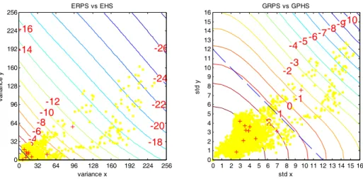
Fig. 3-5 The contour plots of the theoretical WF and the empirical SPF by applying EHS to FB1024 (partial). ... - 24 -

Fig. 3-6 PDF differences between PDFFS(x,y) and SFS(x,y) of CG112. ... - 24 -

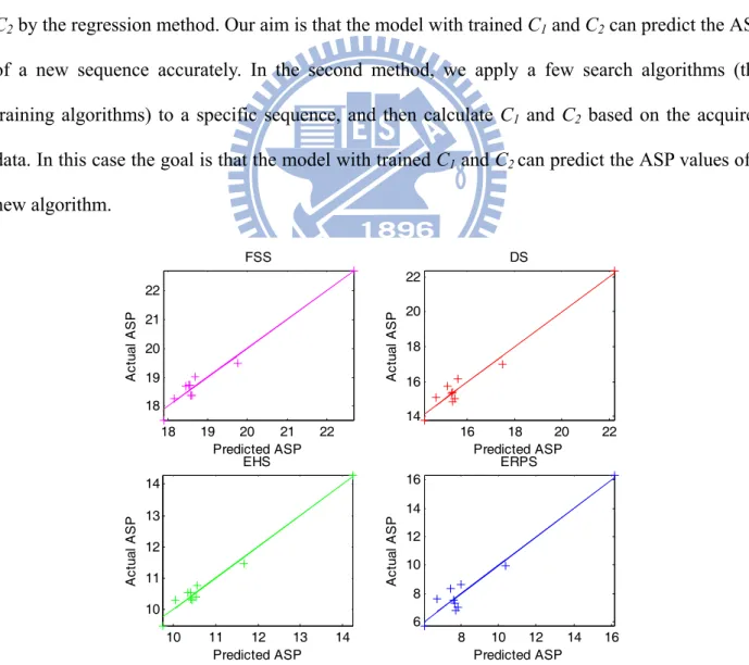
Fig. 3-7 The actual ASP and the predicted ASP pairs for 4 popular search algorithms (1st method)... - 25 -

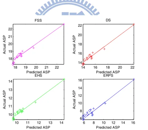
Fig. 3-8 The actual ASP and predicted ASP pairs for 10 training sequences (2nd method)... - 27 -

Fig. 3-9 Search patterns for GRPS... - 29 -

Fig. 3-10 Examples of GRPS search process... - 30 -

Fig. 3-11 WF of GRPS... - 31 -

Fig. 3-12 Relation charts between the predicted ASP and the actual ASP (1st Method)... - 35 -

Fig. 3-13 Performance prediction for GRPS (for various test sequences, 1st method). ... - 36 -

Fig. 3-14 Performance prediction of GRPS as a new search algorithm (2nd method) ... - 37 -

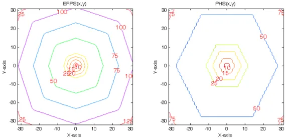
Fig. 4-1 Contour plots of the WFs of ERPS and PHS. ... - 41 -

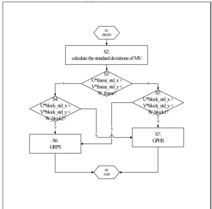
Fig. 4-2 The flowchart of GRPS ... - 44 -

Fig. 4-3 The search patterns for GRPS ... - 45 -

Fig. 4-4 The flow chart of GPHS... - 46 -

Fig. 4-5 The search patterns of GPHS ... - 46 -

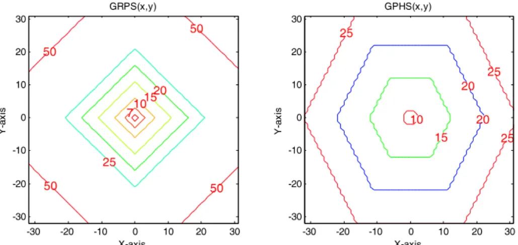
Fig. 4-6 Contour plots of the weighting function for GRPS and GPHS... - 47 -

Fig. 4-7 The IASP between ERPS and PHS w.r.t. MV variance or MV standard deviation, and that between GRPS and GPHS w.r.t. MV variance or MV standard deviation... - 50 -

Fig. 4-8 The flow chart of AGPS. ... - 51 -

Fig. 4-9 Flow chart of the double level adaptive genetic pattern search (DL AGPS)... - 52 -

Fig. 4-10 Pattern switching threshold (dash line), IASP (solid line) and the frame MV variance/STD of the normal sequences... - 56 -

Fig. 4-11 Pattern switching threshold (dash line), IASP (solid line) and the MV variance/STD for the 2X sequences... - 56 -

Fig. 4-12 Motion vector predictor candidates in the current frame, the previous frame and the frame before previous frame. ... - 59 -

Fig. 4-13 The flow chart of constructing SPS... - 61 -

Fig. 4-14 The SAD candidates in the current frame, the previous frame and the frame before the previous frame... - 65 -

Fig. 4-15 Best 2D SAD predictor versus SADC... - 68 -

Fig. 4-16 Best 3D SAD predictor versus SADC... - 69 -

Fig. 4-17 The ASP performances of DS, AIPS-MP and our proposed best algorithm. ... - 75 -

Fig. 4-18 The rate-distortion performances of FS, DS, AIPS-MP and our proposed best algorithm. ... - 75 -

(15)

xi

Fig. 5-2 All possible search sequences for a parent point with N=4 and m=2... - 81 -

Fig. 5-3 Two cases of starting search points, (a) and (b), and two cases of intermediate search points, (c) and (d), in the search process of GRPS when the matching error surface is QMSB. ... - 83 -

Fig. 5-4 The construction of RWF ... - 84 -

Fig. 5-5 The RWF of GRPS ... - 84 -

Fig. 5-6 The real average search points of GRPS when it is applied on the sequence ‘2X MD96’. ... - 85 -

Fig. 5-7 The RWF of GPHS... - 87 -

Fig. 5-8 The RWF of MD-GRPS ... - 89 -

Fig. 5-9 The flow chart of MD-GRPS ... - 89 -

Fig. 5-10 The search priority of all candidate mutations in MD-GRPS. ... - 90 -

Fig. 5-11 The RWF of MD-GPHS ... - 90 -

Fig. 5-12 The flow chart of MD-GPHS ... - 90 -

Fig. 5-13 The search priority of all candidate mutations in MD-GPHS. ... - 90 -

Fig. 5-14 The real average search points of MD-GRPS when it is applied on the sequence ‘2X MD96’. ... - 91 -

Fig. 5-15 Performance comparisons in ASP between MD-GRPS and some popular algorithms.- 95 - Fig. 5-16 Performance comparisons in PSNR between MD-GRPS and some popular algorithms. ... - 95 -

Fig. 5-17 Performance comparisons in ASP between MD-GPHS and some popular algorithms.- 95 - Fig. 5-18 Performance comparisons in PSNR between MD-GPHS and some popular algorithms. ... - 95 -

Fig. 5-19 The relationships between the actual ASP and the predicted ASP for the 1X and 2X sequences... - 98 -

Fig. 5-20 Contour plots of the RWF for FSS, DS, ERPS and PHS. ... - 100 -

Fig. 5-21 Contour plots of the RWF for GRPS and GPHS... - 100 -

Fig. 5-22 The JASP between ERPS and PHS w.r.t. MV variance (a) and that between GRPS and GPHS w.r.t. MV variance (b)... - 102 -

Fig. 5-23 The flow chart of APS. ... - 103 -

Fig. 5-24 Flow chart of the double level adaptive pattern search (DL APS). ... - 105 -

Fig. 5-25 The ASP values of applying ERPS, PHS, APS and DL APS on the 1X, 2X and 4X sequences... - 110 -

Fig. 5-26 The PSNR values of applying FS, ERPS, PHS, APS and DL APS on the 1X, 2X and 4X sequences... - 110 -

Fig. 5-27 The ASP values of applying GRPS, GPHS, AGPS and DL AGPS on the 1X, 2X and 4X sequences... - 111 -

Fig. 5-28 The PSNR values of applying FS, GRPS, GPHS, AGPS and DL AGPS on the 1X, 2X and 4X sequences... - 112 -

Fig. 5-29 The frequency (in percentage) that PHS is chosen when the adaptive pattern schemes, APS and DL APS, are applied to the 1X, 2X and 4X sequences. ... - 113 -

Fig. 5-30 The frequency (in percentage) that GPHS is chosen when the adaptive genetic pattern schemes, AGPS and DL AGPS, are applied to the 1X, 2X and 4X sequences. ... - 113 -

Fig. 5-31 Pattern switching threshold (dash line), JASP (solid line) and the frame MV variance of the 1X, 2X and 4X sequences when the constituent searches are ERPS and PHS. ... - 114 -

Fig. 5-32 Pattern switching threshold (dash line), JASP (solid line) and the frame MV variance of the 1X, 2X and 4X sequences when the constituent searches are GRPS and GPHS... - 114 -

(16)

xii

List of Tables

Table 1-1 The contributions of this dissertation and the related publications ... - 2 -

Table 3-1 The selected training sequences and their settings. ... - 13 -

Table 3-2 Statistic D of 2D KS test... - 17 -

Table 3-3 Parameters of TFS(x,y) for the training sequences and their corresponding KS test results. ... - 18 -

Table 3-4 Regression parameters (C1 and C2) and the correlation coefficients between the model-predicted ASP and the real data. (1st method)... - 26 -

Table 3-5 Regression parameters (C1 and C2) and the correlation coefficients between model-predicted ASP and the actual data (2nd method). ... - 28 -

Table 3-6 ASP (Average number of search points)... - 32 -

Table 3-7 PSNR (Peak Signal Noise Ratio). ... - 32 -

Table 3-8 Coding Performance Comparison. ... - 32 -

Table 3-9 The extra test sequences and their coding settings... - 34 -

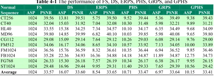
Table 4-1 The performance of FS, DS, ERPS, PHS, GRPS, and GPHS... - 48 -

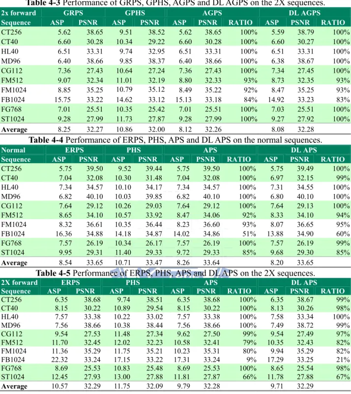
Table 4-2 Performance of GRPS, GPHS, AGPS, and DL AGPS on the normal speed sequences.- 54 - Table 4-3 Performance of GRPS, GPHS, AGPS and DL AGPS on the 2X sequences. ... - 55 -

Table 4-4 Performance of ERPS, PHS, APS and DL APS on the normal sequences... - 55 -

Table 4-5 Performance of ERPS, PHS, APS and DL APS on the 2X sequences. ... - 55 -

Table 4-6 GASP of the MV predictors applied to the test sequences using WFERPS.... - 59 -

Table 4-7 GASP of the MV predictors applied to the test sequences using WFPHS.... - 59 -

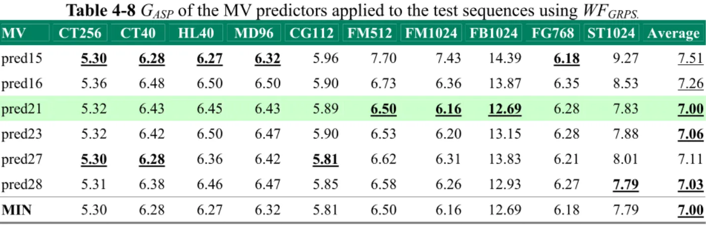
Table 4-8 GASP of the MV predictors applied to the test sequences using WFGRPS.... - 59 -

Table 4-9 GASP of the MV predictors applied to the test sequences using WFGPHS.... - 60 -

Table 4-10 The performance of DL APS with only one starting point... - 61 -

Table 4-11 The performance of DL APS when there are two points in the starting point set. .. - 62 -

Table 4-12 The performance of DL APS when there are three points in the starting point set, MVpred23 is the first starting point, and PMV is the second starting point. ... - 62 -

Table 4-13 The performance of DL AGPS with only one starting point. ... - 62 -

Table 4-14 The performance of DL AGPS when there are two points in the starting point set.- 63 - Table 4-15 The effects of SPS on DL APS and DL AGPS. ... - 63 -

Table 4-16 The correlation coefficients between the selected SAD predictors and the actual block SAD... - 67 -

Table 4-17 Regression coefficients for the best 2D and 3D SAD predictors. ... - 68 -

Table 4-18 The performance of DL AGPS with SPS and various early termination mechanisms.- 70 - Table 4-19 The extra sequences and their settings. ... - 70 -

Table 4-20 The performance of DL AGPS with SSP and various early termination mechanisms on the extra sequences in Table 4-19... - 71 -

Table 4-21 The ASP performance of FS, DS, AIPS-MP, ARPS-ZMP and our proposed best algorithm. ... - 71 -

Table 4-22 The PSNR performance of FS, DS, AIPS-MP, ARPS-ZMP and our proposed best algorithm. ... - 72 -

Table 4-23 The sizes (number of bytes) of the coded bitstreams by FS, DS, AIPS-MP, ARPS-ZMP and our proposed best algorithm... - 72 -

Table 4-24 The rate-distortion test sequences and their settings. ... - 74 -

Table 4-25 The BDPSNR and BDRate comparisons between FS, DS, AIPS-MP and our proposed best algorithm. ... - 76 -

Table 5-1 The ESP values... - 82 -

(17)

xiii

Table 5-3 PSNR (Peak Signal to Noise Ratio). ... - 94 - Table 5-4 The average absolute difference between predicted ASP and actual ASP for all 1X

and 2X sequences... - 98 -

(18)

1

-Chapter 1 Introduction

The explicit use of motion compensation to improve video compression efficiency can be traced back to the late 1960s, a patent filed by Haskell and Limb [1] and a conference paper by Rocca [2], both in the year of 1969 [3]. The necessary operation in the video encoder to enable motion compensation in the video decoder is motion estimation (ME). A technique of motion estimation, block motion estimation (BME), has been widely adopted by the contemporary video coding systems [4][5][6][7] because it is an effective means in reducing the inter-frame correlation for image sequence coding. Block motion estimation schemes partition the current frame into non-overlapping blocks and find the block with the minimal block-matching cost in the reference frame. The most straightforward implementation of BME, the so-called full search (FS), evaluates the matching costs of every motion vector candidate in the search area and finds the motion vector (MV) of the best-matched block. Yet, it requires a huge amount of computing power particularly for sophisticated coding algorithms that include multiple reference frames and variable size block motion estimations. Since 1980s, the pattern-based block motion estimation (PBME) algorithms [17][18][44] have been developed to alleviate the computational burden and to minimize the impact on the coding quality. Static PBME [26][27][28][29][31][32], which use fixed search patterns, got popular in late 1990s and early 2000s. However, because the characteristics of an image sequence vary with time, no one single search pattern can handle the entire sequence well. In 2000s, the adaptive pattern search algorithms [39][40][43], which dynamically switch search patterns, were devised. In this dissertation, we focus only on PBME and its variations.

Section 1.1 Motivation

Despite that many fast algorithms have been proposed to reduce the computational complexity of PBME, most of them are devised based on experimental data or heuristic ideas. Few researchers,

(19)

2

-to our knowledge, have tried -to construct an accurate mathematical model for the PBME process. Therefore, one purpose of this dissertation is to construct an analytical model for PBME, and the other purpose is to design new fast algorithms by using the proposed model.

To be specific, we like to propose a model that reveals the relationship among the video sequences, the search methods, and the computational complexity. Essentially, we want to propose answers to the following questions: Why does one pattern search outperform the other? What is the underlying mechanism of its search efficiency? Is there a pattern search that handles nearly all sequences well? If not, how can we adaptively choose the proper pattern searches? What is the impact of starting points on the coding performance? Is it possible to portray all these problems by using one single model?

Section 1.2 Research Contributions

Table 1-1 The contributions of this dissertation and the related publications Publication

Theory Application

Journal Conference

MV PDF* T.CSVT09[54]*

WF* Genetic pattern searches* T.CSVT09[54]* ISCAS07[51]

Complete Model* Performance prediction* T.CSVT09[54]* 1st Method* Selection of the initial search point set+ T.CSVT10[55] +

2nd Method* Adaptive pattern switching strategy+ T.CSVT10[55] + ICASSP07[52] Optimization of early termination

mechanism+

T.CSVT10[55] +

RWF~ Momentum-directed genetic pattern

searches~

Submitted[56] ~ ICIP08[53] Refined Complete

Model~

Improved prediction accuracy~ Submitted[56] ~

1st Method~ Influences on the selection of starting point set#

Submitted[57] #

2nd Method~ Influences on the pattern switching strategy#

Submitted[57] #

(20)

3

-same superscript marker are published in the -same journal manuscript. Items in the -same row are included in the same conference paper. In the theory part, we build a statistical probability distribution function of the motion vectors (MV PDF) [54], and the minimal number of search points achieved by a pattern-based search algorithm, the so called weighting function (WF) [51]. Combining them together, we propose a statistical model for PBME (The Complete Model) [54]. There are two methods to train the parameters in the model. We further replace the WF by the

refined weighting function (RWF) [53], which better describes the behavior of the probabilistic

PBME. Thus, we have the refined model (Refined Complete Model) [56], which similarly has two training methods to acquire its parameters. In the application part, we devise the genetic pattern searches [51][54] based on our observation of WF. With the complete model, we are able to predict the performance of a search algorithm on an image sequence [54]. Based on the 1st method, we construct the high-performance initial search point set [55]. Based on the 2nd method, we select properly a good threshold for pattern switching mechanism [52][55]. Another application is the optimization of the early termination mechanism. Combining all these tools together, we construct the adaptive pattern search schemes [55]. In addition, hinted by the shape of RWF, we further design the momentum-directed genetic pattern searches [53][56]. With the refined model, the prediction accuracy is improved. Accordingly, we re-examine its influence on the selection of starting point set and the pattern switching strategy [57].

Section 1.3 Dissertation Organization

The rest of this dissertation is organized as follows. First, we review the development of PBME and describe several popular pattern-based search algorithms in Chapter 2. Then, we introduce the model for PBME and present two of its applications – pattern search design and performance prediction - in Chapter 3. Chapter 4 extends the applications of the model to the design of adaptive pattern search schemes, which include three major coding tools – pattern switching

(21)

4

-strategy, starting point selection, and early termination. In Chapter 5, we further refine our proposed model and re-examine all the coding tools in a PBME. Finally, we conclude this dissertation by summarizing our contributions and pointing out some possible future works in Chapter 6.

(22)

5

-Chapter 2 Pattern-based Block Motion Estimation

Modern video compression systems convert the huge digitized video data into a small-size sophisticated bitstream by using the well-known structure – block-based hybrid coding (BHC) [4][5]. A BHC scheme divides an image frame into blocks, reduces the inter-frame dependence among image frames by ME, removes the intra-frame redundancy by intra prediction, discrete cosine transform and entropy coding techniques, and packs the image essential information into a comprehensive representation. In general, a BHC video system comprises two major modules: intra frame coding and inter frame coding. Block Motion Estimation (BME), a ME technique, has been widely adopted by modern video coding standards [4], such as the H.26X series [5] and MPEG-1/2/4 [7].

Although many algorithms have been developed to accelerate BME, however BME remains the most computation-intensive component in the video encoders. As the coding algorithm progresses, the more sophisticated ME tools are invented, such as variable block size ME and multiple reference frames. The most intuitive BME algorithm is FS, which examines all the candidates (checking points) in the search area by calculating the block matching cost between the current block and the reference block and find the motion vector (MV) with the smallest block matching cost. Because FS consumes a tremendous amount of computing power, many researchers have devised fast BME schemes to reduce computation without sacrificing the coding efficiency. According to [8], fast BME algorithms can be classified mainly into two categories: 1) reducing the number of checking (search) points and 2) lowering the computational complexity in calculating the block-matching criterion for each checking (search) point. This dissertation focuses on the algorithms in the first category.

PBME is the most popular scheme in the first fast BME category. It typically consists of three sets of tools for reducing the search points: 1) an operative threshold for early decision

(23)

6

-mechanisms [9][14][30][31], 2) the selection of good initial search points [14][15][16][30][31], and 3) an effective set of search patterns [17][26][27] [28][29][31][32][33]. Combing all these tools, the latest PBME algorithms achieve a dramatic speed-up in finding the near-optimal candidate motion vectors while maintaining a desired level of quality. The first set and the second set of speed-up tools make use of the data correlation inside one frame (intra-frame) or between nearby frames (inter–frame). The third set of tools (search patterns) is effective when the matching cost surface is nearly monotonic. Among these tools, the search pattern plays a key role in deciding the performance of a search algorithm especially when the data correlation is low.

Four step search [26], diamond search [27][28], hexagonal search [29] and their improved versions [30][31][32][33][34], have been the most popular and effective methods in fast PBME. However, since the contents of an image sequence vary quite drastically along with time, one single search pattern often can not handle well the diverse characteristics of the entire sequence. Thus, the adaptive PBME [35][36][37][38][39][40][41][42][43], which mainly comprise multiple pattern searches and a pattern switching mechanism, have been proposed. Note that, the overall performance of an adaptive pattern search algorithm is still bounded by its constituent pattern searches.

Section 2.1 Initial Search Point

The initial search point of the PBME has crucial effect on the search point performance as reported in [14][15][16]. Conventionally, the most common used initial search point is zero motion vector (ZMV, (2.1)) and predicted motion vector (PMV, (2.2)). Herein, we adopt the prediction formula specified by the MPEG-4 standard for PMV. Unless explicitly stated otherwise, we use PMV as the predetermined initial search point for the conventional pattern searches for two reasons. First, the motion vector differences between the best MV and PMV is coded in the bitstream on our simulation platform – a MPEG-4 SP@L3 encoder. That is, when the best MV is

(24)

7

-PMV, it takes 0 bits to code the best MV. Clearly, the simulation platform favors PMV because it consumes the least bits. Second, PMV is likely to be the MV with the smallest block-matching error in statistics. Thus, if we choose PMV as the initial search point, the resulting number of search point acquired by a typical PBME is small. Further discussions on the best initial search points are in Section 4.3.

) 0 , 0 ( = ZMV . (2.1) ) , , (_MVU _MVL _MVUR Median PMV = ,

where the location of MVU/MVL/MVUR and PMV are illustrated by Fig. 2-1. MVU is the adjacent upper block of the current block, MVL is the adjacent left block of the current block, and MVUR is the neighboring up-right block of the current block.

(2.2)

PMV

MV

L

MV

UR

MV

U

Fig. 2-1 Predicted motion vector.

Section 2.2 Some Popular Pattern-based Search Algorithms

Four representative pattern-based search methods, Four Step Search (FSS) [26], Diamond Search (DS) [27][28], Enhanced Hexagonal Search (EHS) [32], and Easy Rhombus Pattern Search (ERPS), are used to illustrate the construction of the PBME model. These pattern-based search algorithms are chosen because of their well-recognized performance. Among the existing PBME algorithms, EHS performs rather well particularly on high motion sequences, and ERPS is more suitable for low motion sequences.

(25)

8 --4 -3 -2 -1 0 1 2 3 4 -4 -3 -2 -1 0 1 2 3 4 -4 -3 -2 -1 0 1 2 3 4 -4 -3 -2 -1 0 1 2 3 4 (a) (b)

Fig. 2-2 Search patterns used in FSS.

-4 -3 -2 - 1 0 1 2 3 4 - 4 - 3 - 2 - 1 0 1 2 3 4 -4 -3 - 2 -1 0 1 2 3 4 -4 -3 -2 -1 0 1 2 3 4 (a) (b)

Fig. 2-3 Search patterns used in DS.

-4 -3 - 2 -1 0 1 2 3 4 -4 -3 -2 -1 0 1 2 3 4 -4 -3 -2 -1 0 1 2 3 4 -4 -3 -2 -1 0 1 2 3 4 (a) (b) -4 -3 -2 -1 0 1 2 3 4 -4 -3 -2 -1 0 1 2 3 4 (c)

Fig. 2-4 Search patterns used in EHS.

-4 -3 -2 - 1 0 1 2 3 4 -4 -3 -2 -1 0 1 2 3 4 (a)

(26)

9

-FSS and DS both consist of two specific search patterns, as shown in Fig. 2-2 and Fig. 2-3, respectively. The large search pattern, Fig. 2-2(a) or Fig. 2-3(a), is used for the coarse regular searches, while the small search pattern, Fig. 2-2(b) or Fig. 2-3(b), is used for fine ending search. Their procedures can be summarized as follows.

Instead of using one single small ending search pattern, EHS uses two small ending search patterns as well as one large coarse regular search pattern as shown in Fig. 2-4. Its algorithm is the same as the one described above except for step 3. EHS switches the large hexagonal search pattern to one of the partial square patterns. The pattern in Fig. 2-4(b) is used when the smallest block distortion sum of two neighboring points in the previous-searched hexagonal pattern is in the vertical direction and the pattern in Fig. 2-4(c) is used otherwise. The two or three points covered by the newly formed partial square pattern are evaluated to compare with the current MBD point, and the new MBD point is the final motion vector.

Unlike other algorithms mentioned above, ERPS uses only one rhombus search pattern in

Fig. 2-5, for both coarse search and fine ending search. This particular rhombus pattern is also

known as “small diamond” in [27][28] and “cross pattern” in [19]. ERPS is a simplified version of Step 1) Check the predetermined starting point, PMV, in the predefined search window, as well as the points in the large pattern, which centers at the predetermined starting point, PMV. If the minimal block distortion (MBD) point is found to be at the center of the large search pattern, proceed to Step 3; otherwise, proceed to Step 2.

Step 2) Set the MBD point in the previous search step as the center, and a new large pattern is formed. New search points generated by the new large pattern are checked if they were not examined in the previous large pattern. Thus, the new MBD point is again identified. If the MBD point is the center point of the latest large search pattern, go to Step 3; otherwise, repeat this step continuously.

Step 3) Switch the search pattern from the large pattern to the small one. The points covered by the small pattern are evaluated to compare with the current MBD point. The new MBD point is the final motion vector.

(27)

10

-adaptive rood pattern search (ARPS[31]). It is ARPS without initial rood patterns as well as various motion vector predictors; PMV is the sole starting search point. The algorithm of ERPS is as follows.

Step 1) Check the predetermined starting point, PMV, in the predefined search window, as well as the points in the rhombus pattern, which centers at the predetermined starting point. If the MBD point is found to be at the center of the rhombus pattern, the MBD point is the final motion vector; otherwise, proceed to Step 2.

Step 2) Set the MBD point in the previous search step as the center, and a new rhombus pattern is formed. Three or two new candidate points are checked, and the MBD point is again identified. If the new MBD point is the center point of the latest rhombus pattern, the new MBD point is the final motion vector; otherwise, repeat this step continuously.

(28)

11

-Chapter 3 Modeling of Pattern-based Block Motion

Estimation

Many researches have proposed fast PBME to reduce the computational requirement of the highly computation-intensive BME. However, few researchers, to our knowledge, have tried to construct an accurate model for the PBME process. To be specific, it is a model that unveils the relationship among the video sequences, the search methods, and the computational complexity. Our aim is to construct an explicit mathematical model for PBME.

Recent research works on PBME often collect the statistics of motion vectors and design good search patterns based on experiences. Few papers are able to provide a systematic way in modeling and designing the search pattern. Among the existing search patterns, the rhombus patterns are known quite effective for low motion sequences [19][20][31], and the hexagonal patterns are very powerful for high motion sequences [29][32][33]. Combining these two sets of search patterns, [21] uses rhombus pattern for initial searches and switches to hexagonal pattern for the succeeding regular searches. One step further, [39] and [40] select the search patterns adaptively according to a set of criteria. Typically these papers use only the experimental data to show the effectiveness of the corresponding search patterns. In this chapter, we like to further explore the following problems. Why does one search pattern outperform the other? What is the underlying mechanism behind it? Is there a search pattern that handles nearly all sequences well? Moreover, can we construct a mathematical model that describes the underlying mechanism? An attempt is made in this chapter to answer these questions.

In this study, we are going to construct a simple and yet effective statistical model for PBME. Using this statistical model, we can predict the performance of one search algorithm when it is applied to a test sequence. Also, based on this model, a novel genetic PBME algorithm is devised.

(29)

12

-distribution functions of the motion vectors acquired by FS. In Section 3.2, we analyze the search points of several representative PBME algorithms and formulate the weighting functions (WF, first mentioned in Section 1.2). Based on the proposed probability distribution function for motion vectors and the WFs of different PBME algorithms, Section 3.3 builds a statistical model for PBME. To demonstrate the use of this model, a new genetic rhombus pattern search is presented in Section 3.4, which shows good performance for both low motion and relative high motion sequences. Section 3.5 describes the second example of using our model: predicting the performance of applying a specific search algorithm to a specific video sequence. Lastly, we summarize this chapter by Section 3.6.

Section 3.1 Probability Distribution of Motion Vectors

In order to design a good search pattern set, many papers discussed the nature of motion vectors. [19], [20] and [21] empirically gather the statistics of the motion vectors around the initial search point and develop their search algorithms. [43] assumes that the motion vector distribution can be approximated by either Gaussian or Laplace probability distributions. So far, we have not found an attempt of inventing a probability distribution function (PDF) that provides a quite precise match to the motion vectors.

We select a few representative training sequences at various bit rates under the settings given in Table 3-1 for generating motion vectors. The selected sequences are encoded by a MPEG-4 SP@L3 encoder using FS. All the sequences are in CIF (352X288) format. Only the first frame is coded as I frame, and all the remaining frames are coded as P frames. The motion vector search range is set to 16, the initial quantizer step size is set to 15, and the block size is set to 16x16. When the quantization step varies to achieve the desired bit rate, the PSNR quality of the coded video sequence ranges from 26dB (poor but acceptable) to 40dB (visually the same as original).

(30)

13

-Table 3-1 The selected training sequences and their settings.

Abbreviation Sequence Bit rate

(K bps) Frame rate(fps) of frames Number PSNR

CT256 container 256 7.5 300 39

CT40 container 40 7.5 300 32

HL40 hall 40 7.5 300 33

MD96 mother and daughter 96 10 300 40

CG112 coastguard 112 30 300 29 FM512 foreman 512 30 300 34 FM1024 foreman 1024 30 300 36 FB1024 football 1024 30 90 35 FG768 flower garden 768 30 250 26 ST1024 Steven 1024 30 300 29

3.1.1 Motion Vector Distributions

Fig. 3-1 Contour plots of the motion vector probability distribution of video sequence CG112

(partial).

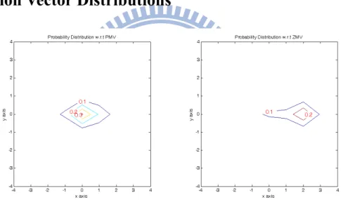
In our experiments, we test two kinds of initial motion vectors (origins of PBME search), namely, ZMV and PMV. Fig. 3-1 shows the probability distributions of the motion vectors obtained by applying FS with a search region [-16~+15, -16~+15] to a video sequence, coast guard at 112K (CG112). Only the probability distribution in region [-4~+4, -4~+4] is shown. The left plot is the motion vector probability distribution with respect to (w.r.t.) PMV, and the right one is the motion vector probability distribution w.r.t. ZMV. Herein, ZMV is defined by (2.1), PMV is defined by (2.2), and the label on the contour shows the probability of motion vectors.

(31)

14

-From the motion vector distributions obtained by applying FS to a video sequence, Fig. 3-1 for example, the motion vector distributions with respect to (w.r.t.) PMV generally have a more symmetric shape as compared to the motion vector distributions w.r.t. ZMV. In addition, the PMV-based motion vectors have a smaller standard deviation. They cluster better. Therefore, the motion vector distribution w.r.t. PMV is thus used in the rest of this chapter.

The statistics of the motion vectors w.r.t. PMV of all the selected training sequences show that the horizontal mean values (μx) and vertical mean values (μy) both are close to zero. Thus,

these motion vector distributions are zero-biased w.r.t. PMV. For a particular sequence, the variance of the horizontal motion vectors (σ2x) is often larger than that of the vertical motion

vectors (σ2y). Furthermore, the correlations (ρxy) between the horizontal components and the

vertical components of motion vectors are nearly zero for all our training sequences in Table 3-1.

3.1.2 Normalized Independent 2D Distribution

Based on the above observations, three popular zero-mean normalized independent 2D distributions are considered as candidates for modeling MV distribution: 1) Gaussian distribution function, 2) Laplace distribution function and 3) Cauchy distribution function.

A Gaussian probability distribution with mean μ and variance σ2 is shown by (3.1); a Laplace probability distribution with mean μ and variance _{2b is shown by (3.2); and a Cauchy}2 probability distribution with median m and the full width at half maximum Γ can be expressed by (3.3), where x∈(−∞,+∞). 2 2 2 ) ( 2 1 2 1 ) ( σ μ πσ − − = x D x e G (3.1) b x D e b x L μ − − = 2 1 ) ( 1 (3.2)

(

)

2 2 1 ) 2 / ( 2 / 1 ) ( Γ + − Γ = m x x CD _π (3.3)

(32)

15

-Because the correlations between the horizontal components of motion vectors, x, and the vertical components of motion vectors, y, are almost zero, it is reasonable to assume that these two random variables in the motion vectors, x and y, are independent. The independent 2D Gaussian probability distribution can be defined as (3.4), where x∈(−∞,+∞) and y∈(−∞,+∞).

2 2 2 2 2 ) ( 2 2 ) ( 2 2 _ 2 1 2 1 ) , ( y y x x y y x x D t independen x y e e G σ μ σ μ

πσ

− − − − = (3.4)

Furthermore, since the mean values of motion vectors are nearly (0,0), one may set

⎪⎩ ⎪ ⎨ ⎧ = = ) , ( ) , ( ) 0 , 0 ( ) , ( 2 2 y x y x y x λ λ σ σ μ μ . Thus, (3.4) becomes (3.5). y x y y x x D x y e e G λ λ πλ πλ 2 2 2 2 2 2 1 2 1 ) , ( = − ⋅ − (3.5)

Although these probability distributions are defined in the domains of x∈(−∞,+∞) and )

, (−∞+∞ ∈

y , the actual distributions of motion vectors are confined in a search area, A.

Consequently, we need to normalize the probability distributions as shown by (3.6). Then, the sum of probabilities in the search area would equal 1.

∑

∈ = A y x D D y x G y x G y x G )' ', ( 2 2 ) ' ,' ( ) , ( ) , ( (3.6) Consequently, the zero-mean normalized independent 2D Gaussian Distribution G(x,y) is defined by (3.7). Similarly, the zero-mean normalized independent 2D Laplace Distribution L(x,y) is defined by (3.8), and the zero-mean normalized independent 2D Cauchy Distribution C(x,y) is defined by (3.9). Note that,(x,y)∈A, and A is the geographical area of [-32~+31, -32~+31] in our

experiments.

∑

∈ − − − − ⋅ ⋅ = A y x y x y x y x y x e e e e y x G )' ,' ( 2 ' 2 ' 2 2 2 2 2 2 ) , ( λ λ λ λ (3.7)

(33)

16

-∑

∈ − − − − = A y x b y b x b y b x y x y x e e e e y x L )' ,' ( ' ' ) , ( _(3.8)

∑

∈ + + + + = A y x _x _y y x y x y x y x C )' ,' ( 2 2 2 2 2 2 2 2 ' 1 ' 1 1 1 ) , ( η η η η (3.9)

Remark: Strictly speaking, the zero correlation between the horizontal components and vertical

components of motion vectors does not imply that they are statistically independent. However,we will justify the correctness of these probabilistic models using the goodness-of-fit test [10][11] as follows.

To find out which of the three PDFs best approximates the PDF of motion vectors acquired by FS, a well-known goodness-of-fit test, 2D KS test [12][13], is adopted. The statistic D defined in [13] is used as the measure of similarity between the hypothesized PDF and the observed PDF (data). To be more specific, the statistic D is the maximum absolute difference between two

cumulative probability distributions. The smaller statistic D is, the better the hypothesized PDF

matches the observed PDF.

In the 2D KS test, the motion vector probability distributions acquired by FS, PDFFS, are

tested against the hypothesized zero-mean normalized independent 2D Gaussian (3.7), Laplace (3.8) and Cauchy distributions (3.9) with the same variances. Therefore, we need to adjust the parameter values of these three distributions so that the variances of the hypothesized distributions equal those of PDFFS. Those fitted hypothesized zero-mean normalized independent 2D Gaussian,

Laplace and Cauchy distributions are called GFS(x,y), LFS(x,y) and CFS(x,y), respectively.

Table 3-2 shows the 2D KS test results between PDFFS(x,y) and the three hypothesized

distributions. Clearly the normalized independent 2D Cauchy distribution CFS(x,y) generally has

(34)

17

-experiments are so large that it is improper to claim that any of these three 2D distributions has a good match to the target PDFFS(x,y).

Table 3-2 Statistic D of 2D KS test.

Sequences GFS(x,y) LFS(x,y) CFS(x,y)

CT256 0.48 0.38 0.08 CT40 0.42 0.35 0.14 HL40 0.36 0.30 0.08 MD96 0.38 0.32 0.12 CG112 0.41 0.32 0.12 FM512 0.39 0.30 0.07 FM1024 0.40 0.30 0.06 FB1024 0.28 0.23 0.19 FG768 0.40 0.32 0.12 ST1024 0.39 0.33 0.17 Average 0.39 0.32 0.11

3.1.3 A Fitted Probability Distribution

To further reduce the difference between CFS(x,y) and PDFFS(x,y), we extend C(x,y) and propose

a new form of PDF denoted by T(x,y), which is defined by (3.10). For each of the selected training sequences, τx and τy are optimized such that the maximum discrepancy between

PDFFS(x,y) and T(x,y) is minimized, and ξx and ξy are adjusted such that the variances of T(x,y)

are the same as those of the training sequences. T(x,y) with those fitted parameters matching the PFDFS(x,y) becomes TFS(x,y). The fitted parameters and their corresponding 2D KS test results

are shown in Table 3-3. One may note that τx and τy vary from 1.13 to 2.2. This indicates the

variations among the test sequences are considerably large.

∑

∈ + + + + = A y x _x _y y x y x y x y x y x y x T )' ,' ( 1 1 1 1 ) , (

ξ

τ τ τ τ (3.10)

(35)

18 -τxand τy generally are around 1.67. We thus choose

⎪⎩ ⎪ ⎨ ⎧ = = ) , ( ) , ( ) 3 5 , 3 5 ( ) , ( y x y x y x ζ ζ ξ ξ τ τ

to simplify T(x,y). The

resultant distribution is called S(x,y) as defined by (3.11).

∑

∈ + + + + = A y x _x _y y x y x y x y x S ) ' ,' ( 5/3 5/3 3 / 5 3 / 5 1 1 1 1 ) , ( ζ ζ ζ ζ (3.11)

Table 3-3 Parameters of TFS(x,y) for the training sequences and their corresponding KS test

results. T(X,Y) CT256 CT40 HL40 MD96 CG112 FM512 FM1024 FB1024 FG768 ST1024 xi_x(ξx) 0.01 0.04 0.13 0.11 0.01 0.25 0.21 0.12 0.09 0.10 xi_y (ξy) 0.03 0.13 0.11 0.10 0.55 0.24 0.20 0.43 0.40 0.19 tau_x (τx) 1.84 1.70 1.73 1.58 1.46 1.94 1.99 1.13 1.75 1.79 tau_y (τy) 1.50 1.54 1.72 1.83 2.21 1.82 1.88 1.18 1.98 1.31 max_pdf_diff 0.01 0.01 0.02 0.01 0.03 0.03 0.03 0.02 0.08 0.01 Statistic D 0.01 0.05 0.06 0.05 0.07 0.05 0.05 0.14 0.12 0.03

The 2D KS test shows that SFS(x,y) on the average has a smaller statistic D in comparison

with GFS(x,y), LFS(x,y), and CFS(x,y). Note that the parameters (ζx, ζy) of SFS(x,y) are obtained by

numerical methods so that the variances of SFS(x,y) match the data statistics. In summary, after

several attempts, we found that SFS(x,y) is a rather good model to describe the probability

distribution of the motion vectors derived by using FS. It constitutes the first element of our complete model.

Section 3.2 Search Points in Pattern-based Search

Algorithms

Search patterns are generally devised based on the assumption that the matching cost surface is a unimodal one; in other words, the distortion associated with a search point closer to the global

(36)

19

-minimum has a smaller value. Under this assumption, the number of search points is defined as the minimal number of search points in all possible paths leading to the best-matched point from the starting (initial) point. The search point number in this definition depends on the search pattern. And, for a given search pattern, it is determined by the shortest path between the initial point and the best-matched point. Therefore, it is a discrete function of the location and will be called

weighting function. By examining the search process of a PBME, we can construct its

corresponding WF.

Note that the global uni-modal cost surface assumption is so strong that it is not always true for most video sequences [32]. Typically it is valid within a small neighborhood of the global minimal point. Consequently, the WF does not represent the actual number of search points. Indeed, it represents the lower bound of the number of search points. But the statistics also show that the number of actual search points is highly correlated with our defined WF.

3.2.1 Weighting Function of Pattern-based Search Algorithms

By examining the search algorithms in Section 2.2, we can construct their WFs. Fig. 3-2 shows two examples of the FSS search process. Fig. 3-2(a) is the case of the minimum search point. There are only two steps. The initial coarse search examines 9 points and the fine ending search examines 8 points. The initial point happens to be the best-matched point. Fig. 3-2(b) shows a typical search process. In addition to the 9 initial search points and the 8 ending search points, FSS checks 3 new points if it moves horizontally or vertically, and it checks 5 new points if it moves diagonally. In the WF of FSS (3.12), ‘9’ represents the coarse initial search points, and ‘8’ represents the fine ending search points. The parameter MFSS(x,y) is ‘5’ if it moves diagonally and

(37)

20 --3 -2 -1 0 1 2 3 -3 -2 -1 0 1 2 3 S (a) 1 1 1 1 1 1 1 1 2 2 2 2 2 2 2 2 4 3 2 1 0 (b) 1 S 2 -1 -2 -3 -4 -8 -7 -6 -5 -4 -3 -2 -1 0 1 2 3 4 5 6 7 8 2 1 3 4 1 1 1 1 1 1 2 2 2 3 3 4 4 4 4 4 4 4

Fig. 3-2 Examples of FSS process.

8 ) , ( ) , ( 9 ) , (x y = +M x y ×n x y + WF_FSS _FSS _FSS (3.12) 4 ) , ( ) , ( 9 ) , (x y = +M x y ×n x y + WF_DS _DS _DS (3.13) ) , ( ) , ( 3 7 ) , (x y n x y K x y

WF_EHS = + × _EHS + _EHS (3.14)

4 ) , ( 1 ) , (x y = +M ×n x y +

WF_ERPS _ERPS _ERPS (3.15)

Likewise, by examining the search steps of the other three PBME algorithms, the WFs of DS, EHS, and ERPS can also be formulated by (3.13), (3.14), and (3.15), respectively. In Eqs (3.13) to (3.15), MDS(x,y) is either 5 or 3, KEHS(x,y) is either 3 or 2, MERPS is either 3 or 2, all depending on

the search direction. And the value of nDS(x,y). nEHS(x,y), and nERPS(x,y) are decided by the

number of movements.

From (3.12) to (3.15), it is clear that in the minimum case ERPS checks only 5 points, while FSS checks 17 points, DS checks 13 points and EHS checks 9 points. Thus, ERPS has the smallest number of search points among the four algorithms for the minimum cases. The minimum cases refer to the situations that the best-matched motion vector is located at the starting point.

Fig. 3-3 shows the contour plots of the WFs of FSS, DS, EHS, and ERPS, respectively. The value on a contour represents the least number of search points for a search algorithm to move from the origin to a point (location) on the contour. Because EHS moves faster than any other

(38)

21

-algorithms, EHS surpasses the other algorithms at distant locations. Therefore, by looking into the WF of a search algorithm, we understand why it works better for a particular situation (fast motion or slow motion). Use ERPS as an example: because WFERPS(x,y) has the smallest values

around the starting point, it has advantages for slow motion situations. On the other extreme, WFEHS(x,y) has the smallest values at distant locations. WF forms the second element of our

complete model.

Fig. 3-3 Contour plots of the WFs of FSS, DS, EHS, and ERPS, respectively.

Section 3.3 Statistical Model for Pattern-based Block Motion

Estimation

Based on the problem formulation in Section 3.1 and Section 3.2, the total average search points (ASP) for a sequence can be represented by (3.16). It depends on both search algorithm (SA) and

(39)

22

-the video sequence. It is -the sum of -the products of -the number of search points and -the motion vector probability distributions at all locations within the search area, where SPFSA(x,y) denotes

the number of search points, PDFSA(x,y) denotes the motion vector distribution acquired by a

specific algorithm, and A is the search area.

∑

∈ × = A y x SA SA x y SPF x y PDF ASP ) , ( ) , ( ) , ( _(3.16)

When we apply a specific algorithm to a specific sequence, we obtain the ASP directly from the experiments without the need of calculating (3.16), which requires the knowledge of

PDFSA(x,y) and SPFSA(x,y). Our goal is to construct a generic model in which the dependency on

SA and video sequence is separable. In other words, the PDF is sequence dependent but not SA dependent. And the search point function is SA dependent but not sequence dependent. That is, we would like to replace PDFSA(x,y) by PDFFS(x,y), and SPFSA(x,y) by WFSA(x,y) in (3.16). Thus,

(3.16) becomes (3.17). Herein, PDFFS(x,y) denotes the PDF of the motion vector acquired by FS,

and WFSA(x,y) denotes the weighting function of a specific algorithm discussed previously. With

(3.17), we can thus predict ASP before actually applying a search algorithm to a video sequence, as long as we know the motion vector PDF acquired by FS and the WF of a specific SA.

∑

∈ × = A y x SA FS x y WF x y PDF ASP ) , ( ) , ( ) , ( _(3.17)

However, (3.17) differs from (3.16) due to a few reasons. First, because the block-matching cost surface typically is not globally monotonic in the search area, the actual search process from time to time does not take the shortest path to the location of the best-matched motion vector. Thus, the average number of actual search points, SPFSA(x,y), is higher than WFSA(x,y), the

shortest-path (minimal) search points. Second, the motion vectors found by a specific algorithm sometimes differ from the ones found by FS. Consequently, the motion vector PDF of this specific algorithm, PDFSA(x,y), is not the identical to that of the full search, PDFFS(x,y).

(40)

23 --30 -20 -10 0 10 20 30 0 0.05 0.1 0.15 0.2 0.25 0.3 0.35 0.4 0.45 x-axis pr obab ilit y CG112 PDF Cross Section PDF_FS PDF_EHS -30 -20 -10 0 10 20 30 0 0.05 0.1 0.15 0.2 0.25 0.3 0.35 0.4 0.45 y-axis pr obab ilit y CG112 PDF Cross Section PDF_FS PDF_EHS

Fig. 3-4 PDF shift between PDF acquired by FS and that acquired by EHS (CG112).

Fig. 3-4 shows the cross sections of PDFs acquired by FS and those acquired by EHS for the video sequence, CG112. It is clear that these two PDFs are not identical. PDF shift refers to the phenomenon that PDFFS(x,y) differs from PDFSA(x,y). The main causes are: 1) the search pattern

is relatively small, thus the search is trapped by a local optimal; 2) the early decision mechanism terminates the search when a near-optimal solution is found; and 3) the starting point of SA disagrees to that of FS, PMV, in our formulation.

Fig. 3-5 shows the theoretical WF and the empirical SPF obtained by applying EHS to the video sequence, FB1024, in the region [-10~+10, -10~+10]. Herein, on the left plot (the theoretical WF), the value on a contour represents the shortest-path search points for EHS to move from the origin to a point (location) on the contour and, on the right plot (the empirical SPF), it represents the average number of actual search points. For the empirical SPF, the contour is not continuous, because some motion vectors never happen when we apply a SA to a specific sequence. Thus there indeed exists some differences between the theoretical WF and the empirical SPF and therefore we called it WF drift. It happens because the search algorithm does not always follow the shortest path in the search process as discussed earlier.

(41)

24 --10 -5 0 5 10 -10 -5 0 5 10 x-axis y-axi s EHS WF 13 17 -10 -5 0 5 10 -10 -5 0 5 10 x-axis y-axi s EHS SPF 13 13 17 25 25 25

Fig. 3-5 The contour plots of the theoretical WF and the empirical SPF by applying EHS to FB1024 (partial). -30 -20 -10 0 10 20 30 0 0.2 0.4 0.6 Y axis P robabi lit y cg112 PDF_FS(x,y) S_FS(x,y) -30 -20 -10 0 10 20 30 0 0.2 0.4 0.6 X axis P robabi lit y PDF_FS(x,y) S_FS(x,y)

Fig. 3-6 PDF differences between PDFFS(x,y) and SFS(x,y) of CG112.

Moreover, Section 3.1 suggests that the distribution S(x,y) best approximates PDFFS(x,y). We

can thus substitute S(x,y) for PDFFS(x,y) in (3.17) as long as its variances are known. Thus, S(x,y)

becomes SFS(x,y), the S(x,y) that matches the motion vectors acquired by FS. However, the

substitution of SFS(x,y) also induces new PDF matching error. Fig. 3-6 shows the PDF differences

between SFS(x,y) and PDFFS(x,y) of the video sequence, CG112.

2 , 1 S (x,y) WF (x,y) C C ASP A y x FS SA + × × =

∑

∈ (3.18)

(42)

25

-Therefore, Eq.(3.17) needs adjustment to compensate for various shifts, drifts and model errors. Eq.(3.18) is a modified formula for modeling ASP. Two additional terms, C1 and C2, are

included in Eq.(3.18). We propose that ASP is a linear function of the sum of the products of

SFS(x,y) and WFSA(x,y). By tuning the values of C1 and C2, we can reduce the WF drift error, the

PDF shift error and the PDF mismatch error. Consequently, with the pre-analysis of WFSA(x,y) for

a specific SA and pre-calculation of SFS(x,y) for a specific sequence, one may use Eq.(3.18) to

estimate the ASP values of another SA when it is applied to this specific sequence.

We need to justify the above model is valid for real data. There are two methods to decide C1

and C2. In the first method, we apply a fixed SA to a set of training sequences to compute C1 and

C2 by the regression method. Our aim is that the model with trained C1 and C2 can predict the ASP

of a new sequence accurately. In the second method, we apply a few search algorithms (the training algorithms) to a specific sequence, and then calculate C1 and C2 based on the acquired

data. In this case the goal is that the model with trained C1 and C2 can predict the ASP values of a

new algorithm. 18 19 20 21 22 18 19 20 21 22 FSS Predicted ASP A ctu al AS P 16 18 20 22 14 16 18 20 22 DS Predicted ASP A ctu al AS P 10 11 12 13 14 10 11 12 13 14 EHS Predicted ASP Ac tu al AS P 8 10 12 14 16 6 8 10 12 14 16 ERPS Predicted ASP Ac tu al AS P

搜尋樣型之區塊移動估計研究：模型、演算法設計與視訊編碼應用

國 立 交 通 大 學

電子工程學系 電子研究所

博 士 論 文

搜尋樣型之區塊移動估計研究：模型、演

算法設計與視訊編碼應用

Pattern-based Block Motion Estimation:

Modeling, Algorithm Design and Video

Coding Applications

研 究 生： 蔡 彰 哲

指導教授： 杭 學 鳴

搜尋樣型之區塊移動估計研究：

模型、演算法設計與視訊編碼應用

Pattern-based Block Motion Estimation:

Modeling, Algorithm Design and Video Coding Applications

研 究 生：蔡 彰 哲 Student: Jang-Jer Tsai

指導教授：杭 學 鳴 博士 Advisor: Dr. Hsueh-Ming Hang

國 立 交 通 大 學

電子工程學系 電子研究所

博 士 論 文

搜尋樣型之區塊移動估計研究：

模型、演算法設計與視訊編碼應用

研究生: 蔡彰哲 指導教授: 杭學鳴 博士

國立交通大學 電子工程學系 電子研究所博士班

摘 要

Pattern-based Block Motion Estimation:

Modeling, Algorithm Design and Video

Coding Applications

Student: Jang-Jer Tsai Advisor: Dr. Hsueh-Ming Hang

Department of Electronics Engineering and Institute of Electronics

National Chiao Tung University

Abstract

Dedication

Acknowledgement

Table of Contents

List of Figures

List of Tables

-Chapter 1 Introduction

Section 1.1 Motivation

Section 1.2 Research Contributions

Section 1.3 Dissertation Organization

-Chapter 2 Pattern-based Block Motion Estimation

Section 2.1 Initial Search Point

PMV

MV

MV

MV

Section 2.2 Some Popular Pattern-based Search Algorithms

-Chapter 3 Modeling of Pattern-based Block Motion

Estimation

Section 3.1 Probability Distribution of Motion Vectors

3.1.1 Motion Vector Distributions

3.1.2 Normalized Independent 2D Distribution

(

)

πσ

πσ

∑

∑

-∑

∑

3.1.3 A Fitted Probability Distribution

∑

ξ

ξ

ξ

ξ

∑

Section 3.2 Search Points in Pattern-based Search

Algorithms

3.2.1 Weighting Function of Pattern-based Search Algorithms

Section 3.3 Statistical Model for Pattern-based Block Motion

Estimation

∑

∑

∑

國立交通大學

電子工程學系電子研究所

博士論文

研究生：蔡彰哲

指導教授：杭學鳴

研究生：蔡彰哲 Student: Jang-Jer Tsai

指導教授：杭學鳴博士 Advisor: Dr. Hsueh-Ming Hang

國立交通大學

電子工程學系電子研究所

博士論文

研究生: 蔡彰哲指導教授: 杭學鳴博士

國立交通大學電子工程學系電子研究所博士班

摘要