a Mobile Robot in
Dynamic Environments
䢇 䢇 䢇 䢇 䢇 䢇 䢇 䢇 䢇 䢇 䢇 䢇 䢇 䢇 䢇 䢇 䢇 䢇 䢇 䢇 䢇 䢇 䢇 䢇 䢇 䢇 䢇 䢇 䢇 䢇 䢇 䢇 䢇 䢇 䢇
Kai-Tai Song,* Charles C. Chang
Department of Electrical and Control Engineering National Chiao Tung University
1001 Ta Hsueh Road,
Hsinchu 300, Taiwan, Republic of China e-mail: ktsong@cc.nctu.edu.tw
Received March 28, 1997; revised July 22, 1998; accepted February 20, 1999
This article presents a design and experimental study of navigation integration of an intelligent mobile robot in dynamic environments. The proposed integration architec-ture is based on the virtual-force concept, by which each navigation resource is assumed to exert a virtual force on the robot. The resultant force determines how the robot will move. Reactive behavior and proactive planning can both be handled in a simple and uniform manner using the proposed integration method. A real-time motion predictor is employed to enable the mobile robot to deal in advance with moving obstacles. A grid map is maintained using on-line sensory data for global path planning, and a bidirectional algorithm is proposed for planning the shortest path for the robot by using updated grid-map information. Therefore, the mobile robot has the capacity to both learn and adapt to variations. To implement the whole navigation system efficiently, a blackboard model is used to coordinate the computation on board the vehicle. Simulation and experimental results are presented to verify the proposed design and demonstrate smooth navigation behavior of the intelligent mobile robot in dynamic environments. 䊚 1999 John Wiley & Sons, Inc.
1. INTRODUCTION
To be useful for accomplishing practical tasks, a mobile robot must be able to navigate smoothly in the real world, where unexpected changes in its surroundings occur. There are many prospective
*To whom all correspondence should be addressed.
applications for such an intelligent, autonomous robot: a few examples include transferring material in automated factories, cleaning in hotels, or deliv-ering meals or patient records in hospitals.1 In such
applications, the robot must reach one or more destinations and perform some kind of task there. While traveling to the destination, it must take care to avoid collisions with various fixed or moving
( ) ( )
Journal of Robotic Systems 16 7 , 387᎐404 1999
Ž . objects such as people or other mobile robots . The sensor-based navigation algorithm is, therefore, very important for using mobile robotic systems.
Early approaches to mobile-robot navigation broke the overall job into subtasks that could be
Ž .
handled by sense-model-plan-act SMPA functional modules. The main problem with such approaches is high computation costs, especially in the percep-tual portions of the systems. Brooks believed that intelligence could be achieved without traditional representation schemes,2 so he proposed a
frame-work called the subsumption system,3 often
re-ferred to as the behavioral system. In Brooks’ approach, navigation was first decomposed into task-achieving behaviors controlled by an algorithm tying sensing and action closely together. Control-system layers were built up to let the robot operate at increasing levels of competence. Although Brooks proposed that intelligence can be achieved without representation, he did not rule out representation and admitted that it is sometimes needed to build and maintain maps.4 For instance, planning a short-est path based on a map can help the robot reach its destination more efficiently. Therefore, researchers have recognized that representational and behav-ioral systems should be combined to deal with more complicated tasks.5
A representational system often plans paths for mobile robots according to a world model. Com-monly used world-modeling approaches include
Ž
grid maps, cell trees, and roadmaps which are .
often constructed from geometric maps . In plan-ning paths, search methods such as AU or bidirec-tional search algorithms can be used in conjunction with these representations. Jarvis6 proposed the
dis-Ž .
tance transform DT methodology for path plan-ning with a grid map. Borenstein and Koren7
pro-posed a vector᎐field᎐histogram method based on a histogramic grid map. The potential field method can work with a world model for path planning, especially with a grid map.8
The behavioral approach lets a mobile robot deal with unexpected obstacles in the immediate environment by using onboard sensory information. This is usually considered a reactive scheme. Re-cently, researchers have been interested in how to prevent robots from colliding with other moving objects. Several methods9᎐ 11 have been proposed to
solve such dynamic motion-planning problems, but most of them have not been actually implemented in real mobile robots. It might be that sensory sys-tems can hardly provide desired motion informa-tion in real time. The frequently used ultrasonic
sensors provide little information and cannot obtain the comprehensive obstacle-motion information re-quired for these proposed reactive navigation meth-ods. CCD cameras provide far more sensory infor-mation, but the longer times required for image processing make real-time operation very difficult. To resolve the sensor-system problem, Chang and Song12 proposed extracting simple implicit motion
information from multiple rangefinders. A neural network predictor was developed to estimate the next-time readings of a ring of ultrasonic sensors. This information is equivalent to the next-time posi-tion of an obstacle’s nearest point relative to the robot. Using such projected information, they pro-posed applying a virtual-force method13 to change
the robot’s motion. This prediction-based virtual-force guidance was found to be quite useful in navigating a mobile robot among multiple moving obstacles.
As can be seen from the description above, there are two different strategies for autonomous navigation: representational and reactive; an opti-mal combination of them is therefore important. Some researchers have proposed using a hierarchi-cal architecture with layers of SMPA modules. Lower SMPA layers provide quicker reaction, and higher layers perform more complicated sensor pro-cessing and world modeling based on lower-layer results. Vandorpe et al.14 developed a hierarchical navigation system in which lower-layer action deci-sions depended on the higher-layer ones. Hu and Brady15 let every control layer generate commands
and then used a command selection module to determine the final motion commands. Stentz and Hebert16 used a weighted average method to
com-bine the results from a global navigator and a local navigator. Some other systems extended the behav-ioral approach by elaborately incorporating suitable representations and planning. Mataric17integrated a
topological representation into a subsumption-based mobile robot. Payton et al.18 transformed an
inter-Ž .
nalized plan a gradient field and reflexive behav-iors into fine-grained actions with activation values. The action with the highest weighted-sum activa-tion value was chosen as the command. Arkin19
Ž used world models to select motor schemes
behav-.
iors . Each schema is associated with a potential field, and the resultant potential navigates the robot. Although integrating reactive navigation and repre-sentation-based planning for intelligent mobile robots has been the object of considerable research attention, no specific approach can yet be recog-nized as being optimal in terms of generality and
effectiveness. Therefore, designing a suitable archi-tecture for integrating the two strategies deserves further attention.
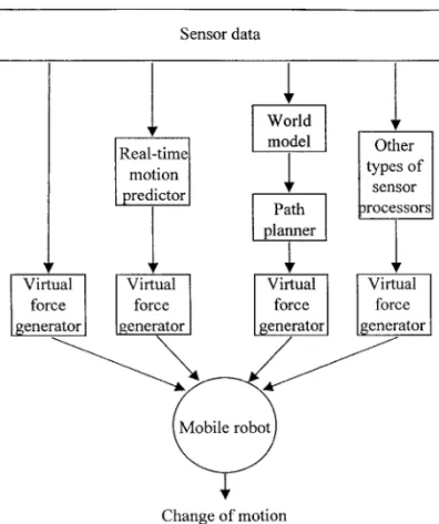
This article presents a new integration method that can navigate a robot in an unstructured envi-ronment, build and update maps, plan and execute actions, and adapt the robot’s behavior to environ-mental changes. The proposed integrated navigation system is based on a virtual-force concept. In this method, navigation resources related to desired be-haviors and constraints are converted to virtual-force
Ž .
sources Fig. 1 . The resultant force changes the robot’s motion to the desired manner. Virtual-force guidance was originally used for reactive naviga-tion in dynamic environments.13 Its principal force
sources come from an ANN sensory predictor,12
which provides implicit information about obsta-cles’ motions. In the integrated navigation system, a path planner is another resource for navigation. Subgoals are extracted from the planned path and each produces a virtual force in sequence. In this article, a bidirectional distance᎐transform method is proposed for path planning. It is based on a grid map that uses a digital filter to fuse sensory data.
Figure 1. Integrated navigation structure using virtual-force concept.
This method is fast and thus aids in developing an on-line path modifier.
The next section presents an efficient method for world modeling. The bidirectional distance᎐ transform method and on-line plan modification are presented in Section 3. Section 4 describes how the virtual-force approach integrates reactive navigation and path planning. Section 5 shows simulation re-sults with an emulated fast mobile robot. Section 6 presents experimental results with a laboratory-con-structed robot, and Section 7 offers the conclusion.
2. GRID MAP BUILDING
A mobile robot should maintain a world model to navigate efficiently. If a mobile robot does not have a map of the external world, it can only react to its immediate surroundings without considering over-all navigational performance. Two types of world models are used extensively: symbolic or categorical representation and analogical representation.20 In
the authors’ system, an analogical representation, a grid map, is used. Grid maps are easy to plan with and maintain.
Grid maps are commonly used with sonar data and maintained by certainty values. In formal prob-abilistic approaches,21, 22 two maps are needed: an occupied map and an empty map. This approach requires much calculation and memory space. Ori-olo et al.23 proposed using fuzzy reasoning instead,
but it also needs two maps. Borenstein and Koren’s method24 is fast, but it considers fewer ultrasonic
sensor characteristics. Song and Chen25 proposed
Ž .
the heuristic asymmetric mapping HAM , a com-promise between computational cost and probabilis-tic meaning.
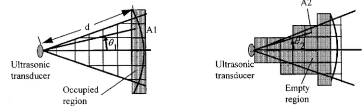
The method described below is extended from the HAM approach and uses a ring of ultrasonic sensors. A cell in the grid map has a value showing the probability of that cell being occupied by an obstacle. The values range fromy1 to 1; the closer to 1 a value is, the more likely the cell is occupied. When an ultrasonic sensor obtains a distance read-ing d, it is very likely that cells within the ultrasonic beam at distances less than d are empty, and cells within the beam at distances around d are occupied. Therefore, empty regions and occupied regions can be represented as shown in Figure 2. The mapping algorithms for cells in these two regions are similar. First, a sensor reading indicates a possibility of a cell in these regions. Then, it is merged into the map through a digital filter to generate a certainty value.
Figure 2. Occupied region and empty region.
For an occupied cell A1, the certainty value given by the k th measurement is given as follows:
Ž . Ž .
gA 1 k sk ⭈k ,d 1 1 where
dyd
¡
min1y for dmin-d-dmax
~
Ž . kds¢
a⭈ dmaxydmin 0 otherwise Ž .2 and 2¡
1 < < 1y for -~
1 m1 Ž . k1sž /
3 b¢
0 otherwise.In the above expressions, d is the raw sensory data, dma x and dmin are the maximum and minimum effective ranges of the ultrasonic sensor, respec-tively, a is a parameter that keeps gA in a desired range, is the angle of cell A1 relative to the1 centerline of the sensor, is the beam angle of theb sensor, and is the maximum angle for admittingm1 occupancy. Value gA1 is then merged into the map
Ž .
to give the certainty value for cell A1 pA1 using a first-order digital filter:
Ž . Ž . Ž . Ž . Ž .
pA 1 k sk ⭈gg 1 A 1 k q 1ykg 1 ⭈pA 1 ky1 , 4 where kg 1 is the weighting factor related to the speed of convergence. Its value must be greater than 0 and less than 1 for convergence.
For the cells in the empty region, negative cer-tainty values are used to represent empty probabili-ties. Two conditions are considered. First, if d-maximum effective range, the certainty value of an
empty cell A2 from k th measurement is
Ž . Ž . gA 2 k syk ⭈k ,d 2 5 where 2
¡
2 < < 1y for -~
2 m 2 Ž . k2sž /
6 b¢
0 otherwise. is the angle of cell A2 relative to the centerline of2
the sensor, and m 2 is the maximum angle for ad-mitting emptiness. The following digital filter is then employed to merge gA2 into the map to give a
Ž .
certainty value for cell A2 in the map pA2 :
Ž . Ž . Ž . Ž . Ž .
pA 2 k sk ⭈gg 2 A 2 k q 1ykg 2 ⭈pA 2 ky1 7 where kg 2 is the weighting factor in the empty region. Second, if dGmaximum range, it means that there is either no obstacle in the detection area or that a specular reflection has occurred. Considering
Ž .
that it may be a specular reflection erroneous data , a modified formula must be used to update the cell-certainty value:
Ž . Ž . Ž . Ž . Ž .
pA 2 k sk ⭈gg 3 A 2 k q 1ykg 3 ⭈pA 2 ky1 , 8
where kg 3 is a weight factor smaller than k .g 2 The following considerations have been taken into account in designing the parameters in these formulas.
1. k , the distance factor. Normally, a speculard reflection leads to a measured distance greater than the actual distance. Therefore, the credit must be smaller when the mea-sured distance is larger. Thus, k is set to ad
Ž
and gA2 is from y0.4 to y0.1 where the value 0.4 is the threshold for distinguishing
. whether or not a cell is occupied .
2. k1 and k , the direction factors. An object is2 easier to detect when it is located in the Ž . centerline of the ultrasonic beam. Eqs. 3
Ž .
and 6 reflect this fact.
3. k , k , and k , the weighting factors. Theg 1 g 2 g 3
weighting factor is related to the conver-gence of the digital filter. The smaller the value is, the slower the convergence speed. A computer simulation was used to deter-mine suitable values. If one takes 0.7 as the average certainty value for occupied cells and -0.7 as that for empty cells, then one’s design goal can be set as follows: four con-secutive data that indicate occupancy with the average certainty values will change an empty cell into an occupied cell. This can be
Ž .
checked by employing 4 . Solving this equa-tion by the numerical method, one finds that kg 1 is about 0.35. On the other hand, the authors hope for three consecutive data that indicate emptiness will change an occupied cell into an empty cell. Similarly, kg 2 is found to be about 0.09 and kg 3 0.022. Note that a preference for an empty cell is adopted in this design, allowing more free space for path planning.
This digital filter reasonably interprets current as well as historical sensory data. Past measured data also contribute to the cell’s current certainty value. However, the present measurement takes rel-atively higher weight, while the older ones will finally take nearly zero weights. The formal struc-ture of traditional filters, such as Kalman or Wiener filters, is not adopted here. The authors’ structure is more heuristic to match the characteristics of the sensor employed. This is also simpler compared with the formal structures. Furthermore, the Gauss-ian noise premise for Kalman filters does not exist in the dynamic environment. For instance, a for-merly occupied cell may be identified as being empty simply because the obstacle has moved away. This map-building method can be used with other types of sensors which give range information about obstacles. However, because of different sen-sor models, the parameters discussed above should be modified. One merit of this present design is that its grid map does not record moving obstacles since they do not stay at fixed locations very long. It can
Ž .
be seen from 4 that the digital filter does not allow one or two sensor inputs to elevate the cell certainty value so high as to change its status. After moving obstacles have passed, the cell values decrease be-cause the next sensor inputs indicate the absence.
Ž
Recording only static obstacles which may change .
positions, however fulfills navigational require-ments because moving obstacles do not stay at fixed locations and should not affect path planning.
3. PATH PLANNING AND PLAN MODIFICATION
In this integrated design, the path planner works to provide a reference path for the robot to travel to the goal according to the current grid map. The planned path is suboptimal in terms of distance. Before path planning begins, the grid map is first divided into occupied and empty areas, according to the 0.4 threshold value. This produces a binary map. Then, occupied areas are expanded by the radius of the mobile robot. This simplifies the path planning problem to a point on the map. The next section proposes a path planning method using the DT concept.
3.1. Path Planning Using Bidirectional Distance Transform
Distance transform is essentially the propagation of Ž
distance away from a set of core cells zero-distant .
from themselves in a tessellated space. For robot path planning, this propagation flows around
obsta-Ž .
cles occupied areas from the start or goal posi-tions. In a 2-dimensional representation, each cell has eight neighboring cells to propagate the dis-tance. The global distance of a cell from the core cell is computed from the local distance between two neighbors. The distance between horizontalrvertical neighbors is denoted d1, and the distance between diagonal neighbors is denoted d2. Different distance proportions between d1 and d2 have been utilized. Borgefors26 found that when d2rd1 equals about
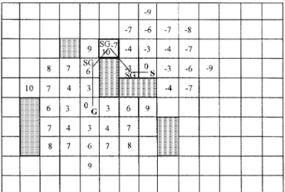
1.351, the error between the transformed distance and the Euclidean one has a minimum upper bound. In the authors’ method, d1 and d2 are set to integers 3 and 4, respectively, to speed up computa-tion. Bidirectional DT, in which distances are propa-gated simultaneously from the robot’s position and the goal, is proposed to cut both search space and computation time by about half. The DT from the goal takes positive values, while the DT from the
robot’s position takes negative ones. When a cell is marked as having positive and negative values, it is termed a meet cell and the propagation stops. The shortest path can be found by backtracking from the meet cell to the robot’s position and goal using steepest gradient ascent and descent algorithms, respectively. Figure 3a shows an example of path planning employing bidirectional DT. In this figure, distances are propagated from S and G, where S denotes the robot’s start position and G denotes the goal position. The propagation stops at the bold-lined cell, which is marked as having both positive and negative values. Subgoals, which are the turn-ing points of the path and denoted by SG, should be extracted because they will be used for integration
Ž .
with reactive navigation see next section . Note that the extraction of subgoals can be realized in the
Ž .
Figure 3. a An example of bidirectional DT-based plan-Ž .
ning. b An example of plan modification when previous plan is found to be improper.
backtracking phase with little extra computational loading.
3.2. On-Line Plan Modification
The preplanned path may become invalid because the environment may change after the robot moves. If this variation is considerable, replanning is often the best policy, although reactive navigation may also be able to maneuver the robot to the goal. Nevertheless, complete replanning requires too much calculation and is not preferable. Stentz27
pro-posed a DU algorithm that can amend improper plans resulting from the environment changes; how-ever, the algorithm itself is much more complicated than the DT-based approaches. Vandorpe et al.14
adopted a reactive planner that uses a DT-based approach within a local window covering two
con-Ž .
secutive intermediate via-points subgoals . Their method costs too much computation time because the reactive planner must be applied repeatedly. Even so, it still is not guaranteed to produce the best plan because of the limited search window.
This article’s plan modification method utilizes information from the original plan since most of the world model remains the same except for the local changes detected by the sensors. In the original
Ž .
plan, numbers distances marked in the cells by applying DT from the goal are still valid if they are not larger than the positive numbers in the changed parts of cells. If all the changed cells have negative numbers, then all the positive numbers marked by the original plan remain valid. To amend the plan, it
Ž .
is only necessary to 1 clear improperly marked numbers, including the negative ones marked by DT from the robot’s start position and positive ones that are greater than the smallest positive numbers
Ž .
of the changed cells and 2 propagate the negative number from the robot’s current position to a cell with a positive value previously marked by DT from the goal. Figure 3b shows an example of path modification, in which a new obstacle is found on
Ž .
the previously planned path Fig. 3a . In this case, the new obstacle occupies cells that were marked with 9 and 10, so the cells marked with 10 are cleared. All cells with negative numbers are also cleared. Then negative DT numbers propagate from the robot’s current position until it reaches a cell with a positive value. The replanned path is there-fore updated. This plan modification scheme pro-vides the shortest path and requires much less com-putation time than does complete replanning.
Because of the limitation of motion directions, path planning using the DT-based approach is in-herently crude. To boost navigation performance while cutting traveling distance, check if there is a clear path between the robot’s current position and the next subgoal. If the path is free from obstacles, then the robot discards the current subgoal and moves toward the next one. This way one can make up for the movement direction limitations.
4. INTEGRATION WITH REACTIVE NAVIGATION
It is desirable for the path planner to be integrated with a reactive scheme that responds to immediate obstacles to make a complete navigation system. There are, however, two problems in performing
Ž .
this integration: 1 the command formats are differ-Ž .
ent; and 2 the proactive and reactive navigation methods are totally independent. This section pro-poses the virtual-force method to solve both prob-lems. First, the planned path and reactive behaviors are transformed into virtual forces exerted on the mobile robot. Then, the two types of navigation can be merged by calculating the resultant force. This force determines the way the robot changes its mo-tion according to Newton’s second law of momo-tion. Because the relationship between force and motion change is obvious, it is easy to design forces to match desired behaviors. In the present system, virtual forces are designed so they can deal with intelligent but possibly careless moving obstacles. This means that the moving obstacle itself can take half the responsibility for preventing collision, but might not do so because of carelessness. Moreover, if any new navigational resources are added or new behaviors desired, appropriate virtual forces can be created and added to the system. The following paragraph introduces the virtual forces for reactive navigation. Then, integration with the planned path is presented.
4.1. Virtual Force for Reactive Navigation
It is important for an intelligent mobile robot to react to previously unrecorded obstacles in the im-mediate environment. Moreover, to cope with mov-ing obstacles, the robot needs to know their motions to avoid them safely. The authors’ mobile robot is equipped with a ring of 16 equally spaced ultra-sonic rangefinders for detecting obstacles. These sensors are fired sequentially in four groups. The
Ž .
error-eliminating-rapid-ultrasonic-firing EERUF method proposed by Borenstein and Koren28 was
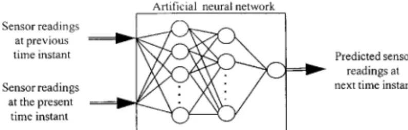
adopted for this study. A complete set of 16 sensor measurements takes only 140 ms. However, range-finders have difficulty identifying obstacles, and their motion estimation will have large degrees of uncertainty. In the authors’ reactive navigation scheme, rangefinders are not used to identify the precise shapes and positions of obstacles. Instead, the sensory system only tells the robot what area will be occupied by obstacles. This is an implicit form of considering the motions of obstacles. Such information can be obtained by predicting future sensor readings employing an artificial neural net-work.12 The authors’ prediction theorem is based on
the knowledge that the measurement from any given sensor must have a relationship to historical mea-surements from sensors nearby. As illustrated in Figure 4, sensor readings of present and previous sample instants are sufficient to predict the next
Ž one. Raw data from four neighboring sensors two
.
on the left and two on the right and the given sensor itself are used to predict next-time sensor reading. Since the mobile robot is equipped with a ring of 16 ultrasonic sensors, the entire predictor is constructed from 16 identical ANNs. The ANN was trained off-line using training data generated by an environment-configuration simulator. At the run time, the ANNs predict future sensory data on-line in real time. Thus, future positions of obstacles are used to form virtual-force sources to let the robot respond to anticipated changes in environment.
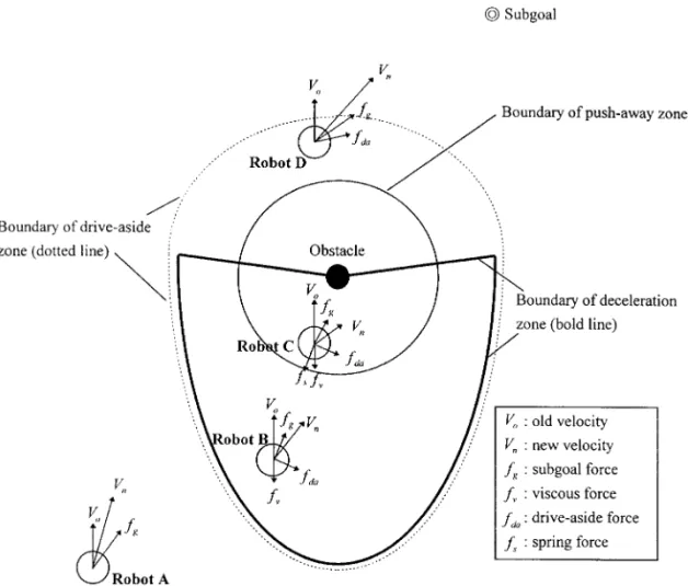
In this design, it is assumed that a point obsta-cle is located in the sensory direction and at the predicted distance. For each obstacle, three force zones were established around it. When the robot enters these zones, virtual forces will be generated to make it behave in a certain manner. The resultant force is determined to change the robot’s velocity and make it easily. avoid moving and static obsta-cles.
The first force zone around an obstacle is termed the deceleration zone. In it, the robot decreases its
speed. It is usually desirable that the robot de-creases its speed to a certain range within a preset time interval. Consequently, viscous force is a suit-able choice in such a situation because it has the effect of decreasing the robot’s speed in proportion to its current speed. Note that even when the robot is at a location covered by the deceleration zones of many obstacles, it is sufficient to count only one viscous force.
The second force zone is the push-away zone. When the robot somehow gets closer to an obstacle, it is necessary to exert a relatively large force against it to prevent a collision. Eventually the force will be large enough to push the robot away from the obstacle. A virtual spring installed between the robot and the obstacle is suitable for this purpose because the spring force exerted on the robot directs it away from the obstacle. Consequently, as the robot pen-etrates deeper into the push-away zone, an
in-creasing push-away force will exert against it. By properly choosing the spring constant, this force guarantees the robot will never collide with a static obstacle.
The third force zone around an obstacle is the drive-aside zone, which makes the robot avoid moving obstacles moving toward it. This force also helps to avoid static obstacles more smoothly. The virtual force generated in this zone, which is termed the drive-aside force, drives the robot away in a lateral direction. Note that a drive-aside action can make the robot move left or right. The robot will choose the one that will move closer to the goal. Figure 5 depicts the forces that affect the robot’s motion in different zones. The extents of three force zones around an obstacle can be seen in this figure. The virtual force strength should be determined according to the kinematic parameters of the mobile robot. The kinematic constraints for this study’s
Figure 5. Virtual forces used for the integrated navigation: subgoal force works every-where, but may be suppressed; three forces from obstacles work within the correspond-ing zones. Robots receive different forces in different areas. Robot A is far away from the obstacle; only the subgoal force affects it. Robot B is in the deceleration and drive-aside zones of the obstacle; subgoal force is suppressed. Robot C is in the push-away, deceleration, and drive-aside zones of the obstacle; subgoal force is also suppressed. Robot D is in the drive-aside zone of the obstacle; subgoal force is not suppressed here.
experimental robot, which has two drive wheels,
Ž .
include maximum wheel speeds vma x , maximum
Ž .
speed change ␦ vma x during a sampling period ŽT , and maximum speed difference between thes.
Ž .
two drive wheels ⌬vd, max . Thus, these constraints are adopted as references when the virtual force system is designed. During derivation of the virtual force parameters, the SI unit system was used. However, the system can be more easily described by simplifying the correlation between the force and the motion command. Denoting the robot’s velocity change during a sampling period as ␦ v, the mass of the robot as m, and the acceleration as a, the force is then ␦ v Ž . fsmasm 9 Ts Ts Ž . ␦ vs f . 10 m
One can correlate the force with the velocity by properly assigning units of virtual force such that
Ž .
␦ vsF, 11
where F is the measure of force in the newly as-signed unit.
The range of force zones depends on the robot’s motion capacity and can be set by the designer. The virtual viscosity coefficient and the spring constant are determined in an iterative manner. The drive-aside force lets the robot detour around obstacles. Its strength must be large enough to move the robot a safe distance away from its original path before the robot is too close to an obstacle. Notably, the range of each zone is expressed in terms of the predicted distances between the robot and obstacles. Thus, appropriate parameters are selected, and the resultant virtual force can guide the mobile robot through a dynamic environment. When there is no obstacle around, the robot is drawn to the goal Žsubgoal by goal force. When it encounters an ob-. stacle, the viscous force makes it slow down so it can react smoothly to prevent a collision. The spring force guarantees that the robot does not collide with an obstacle. If necessary, it will run away from the obstacle. The drive-aside force makes the robot edge off the set path to avoid an obstacle on the way. If there is more than one obstacle, the drive-aside forces from different obstacles will cancel each other if they are contradictory. Spring force from different obstacles all push the robot away, so the resultant
force will guide the robot toward a free space, if one exists.
4.2. Virtual Force for Planned Paths
In an integrated navigation system, a planned path can help the mobile robot reach its destination more efficiently. However, the planned path cannot al-ways be followed exactly because the environment is dynamic and the robot has to avoid unexpect-ed obstacles. Consequently, in this approach the planned path is used simply as a guide from which subgoals are extracted. The mobile robot only needs
Ž .
to almost reach each subgoal in sequence; in be-tween, the trajectory can be flexible to avoid unex-pected moving and stationary obstacles. In general, the mobile robot can still reach the destination along a suboptimal yet short route. Thus, the plan is employed to provide sequential subgoals which pull the robot with virtual force.
When the robot arrives at a subgoal has a clear path to the next one, the next subgoal is then taken into the virtual force guidance system. The subgoal force is designed according to situations encoun-tered. When no obstacle is predicted to be around the robot, this force can take any desired form. Normally a constant attraction is suitable. When the robot is close to a subgoal, the force is designed to navigate it toward the subgoal at a moderate speed so it will move smoothly from the current subgoal to the next one. On the other hand, when an obsta-cle is predicted to be close to the robot’s course toward the subgoal, the subgoal attraction will be suppressed by a decay factor. This factor is deter-mined by the angle measured from the robot’s cur-rent position to the locations of the obstacle and subgoal. Examples of the normal and suppressed subgoal forces are shown in Figure 5.
5. SIMULATION RESULTS
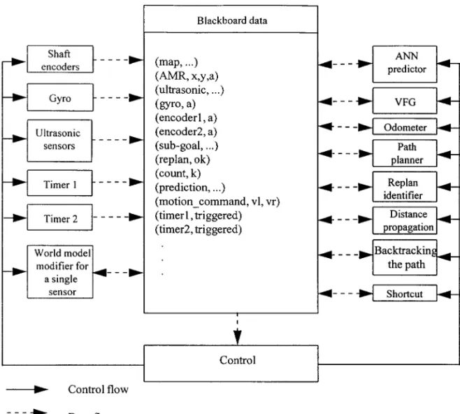
Figure 6 illustrates the blackboard system for imple-mentation of the proposed navigation integration. A blackboard system29 inherently uses its knowledge
Ž .
sources KSs very flexibly. In this application, sen-sors are regarded as KSs, and the sensory data can be employed easily for various functions. This archi-tecture coordinates different functions, including new functions in the future work. The blackboard in the middle of the figure holds computational and current-state data needed by and produced by the
Ž .
Figure 6. The blackboard structure for navigation realization.
data are represented as attribute᎐data pairs. The KSs on the two sides of the blackboard are sets of domain knowledge used to solve subproblems in navigation. They are dispatched by an event-based
Ž .
control module see the control-flow paths accord-ing to the states shown in the blackboard.
Computer simulations have been carried out to verify the integrated navigation performance. The simulated mobile robot is cylindrical with a radius of 30 cm. It is equipped with a ring of 24 ultrasonic sensors, each having a beam opening angle of 22.5⬚ and an effective range from 30 to 600 cm. The simulated sensor reading is the nearest distance to an obstacle within the sensor’s beam angle, zero-mean Gaussian noise with 1% distance-proportional standard deviation plus 1 cm standard deviation.30
Specular reflection is also simulated. It occurs when the wave incident angle is larger than 23⬚. In this case, the ultrasonic wave may echo back after multi-ple reflections or may not come back at all, which
depends on the configuration of obstacles around. However, because it is difficult to model the actual specular reflection among real-world objects, the authors adopted a stochastic model according to their experimental data. It is assumed that there is a 10% chance the distance measurement is the real one multiplied by a random number with a Gauss-ian distribution of mean 3.5 cm and standard devia-tion 0.5 cm and a 90% chance the measurement is the maximum sensing range. In the simulation, the robot’s maximum speed is 200 cmrs, but it is lim-ited to 160 cmrs when not avoiding an obstacle. The sampling time for navigation is 500 ms. The simulation results presented below are for an indoor environment measuring 33=21 m.
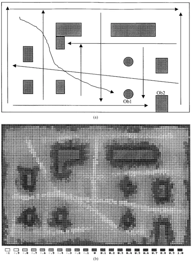
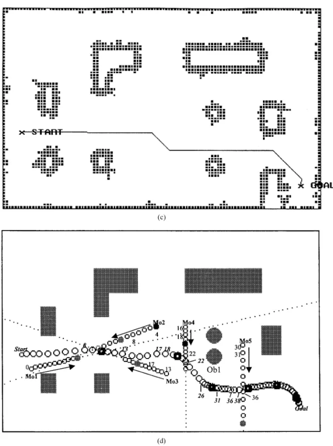
The simulation environment is depicted in Fig-ure 7a, which originally was not recorded for the mobile robot. Given 11 reference paths as shown in the figure, the robot moved along these paths em-ploying the integrated navigation system four times.
It then built the world model shown in Figure 7b from learning. Figure 7c depicts a path planned for a given task based on the binary map. Note that in Figure 7d, five moving obstacles denoted by Mo1 to Mo5 appeared, static obstacle Ob1 changed its
posi-tion, and the originally recorded Ob2 disappeared. In Figure 7d, the positions of the robot and moving obstacles are depicted in black and gray circles, respectively, at every sampling instant. The robot positions at every 10 samples are depicted in solid
Figure 7. Simulation showing that the integrated system can build and update maps, Ž .
deal with moving obstacles, and adapt to environmental changes. a Original environ-Ž .
ment and exploration path. b World model built on-line for the originally unknown environment.
lines. The numbers in the figure indicate the sam-pling moments at which the positions of the robot and moving obstacles were recorded.
The robot first accelerated to pass Mo1 because of goal attraction and the drive-aside force from
Mo1. Note that the robot found there were straight clear paths to the second and third subgoals at the first and second sampling instants, so the source of subgoal-force moved to the second and third sub-goals. At the 8th sampling instant, the force from
Ž . Ž .
Figure 7. c Initial planned path. d Trajectory of motion shows the robot can avoid Ž
moving as well as static obstacles smoothly and safely speed of Mo1 was 100 cmrs, of Mo2 was 130 cmrs, of Mo3 was 90 cmrs, of Mo4 was 88 cmrs, and of Mo5 was 165
. cmrs .
Mo2 made the robot turn right. At the 13th sam-pling instant, the force from Mo3 made the robot turn left to prevent a collision with Mo3. At the 17th sampling instant, the robot passed Mo3 and turned back toward the third subgoal. At the 18th sampling
instant, Mo4 was predicted to be in the robot’s path, and its force made the robot begin to turn right to pass it. At the 22nd sampling instant, the drive-aside force from Mo4 accelerated the robot so it left Mo4’s course quickly. The robot continued curving around
Ž .
Figure 7. e Updated world model, from which the tracks of moving obstacles can be
Ž . Ž .
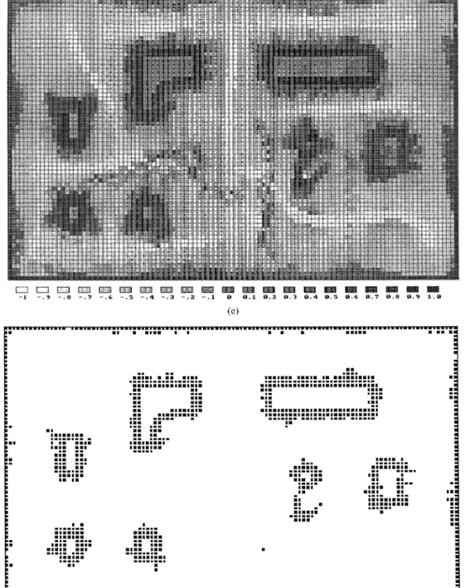
the circular obstacle Ob1. The plan was modified around this area, and the robot slowed down at the 26th sampling instant because it was close to a newly planned subgoal. At the 31st sampling in-stant, Mo5 was predicted to be in the robot’s path, and the robot turned right to avoid it. However, unlike when it met Mo4, before it could move fast, Mo5 suddenly intruded and then passed its course. At the 36th sampling instant, it turned slightly left to avoid Mo5. After the 38th sampling instant, the robot moved toward the goal smoothly. Figure 7e depicts the updated map, in which Ob1’s position had been corrected and Ob2 had been eliminated, as expected. The tracks of moving obstacles can be seen on the grid map, but they are invisible on the
Ž .
binary map Fig. 7f .
In this simulation, the robot controlled its mov-ing direction and speed so well that it was close to a human’s behavior. It accelerated to pass slow obsta-cle Mo1, took slight turns to keep safe distances from Mo2 and Mo3, took a sharp turn to avoid oncoming obstacle Mo4 and static Ob1, then re-planned its path, and finally decelerated to wait for quick Mo5 pass. The whole path was so smooth and nearly every turn or speed change was necessary. Humans with the same sensing capability could hardly do better.
6. EXPERIMENTAL RESULTS
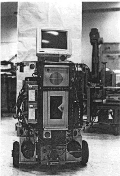
Figure 8 shows the experimental mobile robot de-veloped in the authors’ laboratory. Its diameter is 60 cm and it is about 110 cm high. It has two indepen-dent drive wheels and two casters for balance. Its maximum speed is 40 cmrs. A ring of 16 ultrasonic sensors is installed around it at alternating heights of 30 cm and 75 cm with equal angle spans. The effective range of each sensor is 43 to 300 cm. A cycle of all 16 ultrasonic sensor measurements takes about 140 ms. The sampling time for a navigation command is 560 ms. Two encoders attached to the drive wheels and a gyroscope are used for self-localization. The control and computation tasks are
Ž
distributed among two HCTL-1100s for servo
mo-. Ž
tor control , an Intel 8751 for ultrasonic sensor
. Ž
measurements , and an Intel 80486-33 for other .
tasks .
The experiments were conducted in corridor of Ž the authors’ laboratory. Only part of the floor 33=
.
12 m was utilized in the experiments, and its origi-nal map is as shown in Figure 9a. This is a simpli-fied map in which the details of doors and objects
Figure 8. Picture of the experimental mobile robot.
are not illustrated. Figure 9a also shows a path planned in corridors for a given task. Note that there was a long wall in the goal direction at the beginning. The robot could hardly attain its goal without the plan because the goal attraction would be canceled by the virtual forces from the wall.
Ž Three previously unrecorded static obstacles
car-. Ž .
tons and two moving obstacles persons were pre-sent in the experimental environment. Ob3 just blocked the preplanned path. A static obstacle recorded in the previous map had been taken away. Figure 9b illustrates the trajectories of the robot and moving obstacles. Because the speeds of the robot and moving obstacles were relatively low, depicting their positions every sampling instant would be too dense to read. The authors depicted every 4th sam-pling instant and with dark shading every 20th sampling instant, to make them easier to read.
In the beginning, the robot moved toward its first subgoal. A slight directional change occurred at
Ž the 4th sampling instant due to a door frame
prom-.
to 92nd sampling instants, the robot smoothly passed a slowly moving person. From the 108th to 144th sampling instants, it moved along a straight line at a constant speed in the corridor, a difficult task for general potential field methods. The virtual
force system is able to do this because each force is associated with a behavior, and therefore it is easier to design appropriate force. It is also worth noting that the trajectory of the robot during this stage was farther away from the wall than the preplanned
Figure 9. Experiment showing that the mobile robot can deal with unexpected obstacles Ž .
and update its world model in real-time operation. a Initial world model and planned Ž .
path. b Trajectory of motion showing the robot avoiding unexpected moving and static
Ž Ž .
obstacles smoothly speed of Mo1 was 14 cmrs and of Mo2 was 36 cmrs. c Updated grid map, in which previously unknown obstacles are reported.
path, resulting in safe navigation. The robot turned right at the 144th sampling instant because of a closed door at its left front. It then traveled around Ob2 and Ob3 through the middle of the free area. At the 196th sampling instant, the robot began turn-ing right because of Mo2. However, Mo2 moved fast, and the robot had no chance to move toward the goal in front of Mo2. Consequently, it began to turn left again at the 208th sampling instant and then moved toward the goal after Mo2 no longer blocked its path. The updated map is depicted in Figure 9c. Figure 10a shows the binary map con-verted from Figure 9c. It was observed that three previously unknown static obstacles were recorded, and an old static obstacle had been removed from the map because it was not present in the environ-ment. The closed doors were also perceived. Part of Mo1’s track was recorded in the map because it moved slowly. However, this was only temporary.
Continuing the experiment, this time the robot traveled back to the previous starting point. The
Ž .
planned path Fig. 10a was not blocked by any position-changed static obstacles. With this correct plan resulting from map-learning, the robot moved faster than its previous journey, especially when
Ž .
traveling around Ob3 Fig. 10b . At the 84th sam-pling instant, the robot predicted Mo1 would be close and turned left to avoid it. Mo2 came along later, and the robot turned right to avoid it at the 104th sampling instant. Because the robot had been very close to Mo1 and Mo2, the spring force from Mo1 and Mo2 pushed it away at the 92nd and 112th sampling instants, respectively. After the robot passed Mo2, it traveled smoothly to the goal. Note that, without the reactive part, the robot would have collided with the moving obstacles. The up-dated map is shown in Figure 10c and 10d. Note that the track of Mo1 in the last experiment has
Figure 10. Experimental results showing the mobile robot moves faster around a recorded obstacle because the reference path was planned according to the updated
Ž . Ž .
world model. a Initial planned path. b Trajectory of motion showing the mobile robot moving faster around Ob3 after it learned the new environment. Also shown are different
Ž
Ž .
Figure 10. c Updated world model from which the track of the slowly moving obstacle
Ž . Ž .
in the previous experiment has been removed. d Binary map converted from c .
disappeared. This experiment reveals that the robot can navigate safely and smoothly in a dynamic environment. The proactive and reactive navigation algorithms are integrated to give satisfactory re-sults. Because of the accumulated errors, the posi-tioning errors at the final positions in this round-trip experiment were 15 and 17 cm, respectively. A landmark approach can be employed to compensate for this accumulated error. Compared to the travel-ing distance over 30 m, these small errors implied that the robot can run a long distance without losing its position if only a few landmarks are available.
7. CONCLUSIONS
This paper presents an integrated navigation system for an intelligent autonomous mobile robot in dy-namic environments. A new method is proposed for
integrating local reactive navigation with a proac-tive plan. This method is based on the virtual-force concept, which assumes that each navigational re-source exerts virtual force on the robot to produce desired motion changes. This approach has the ad-vantage of integrating various resources with differ-ent degrees of abstraction in a uniform manner. To deal with moving obstacles, a real-time sensory predictor is used so that the robot can react to environmental changes more efficiently. A grid map is maintained for path planning by using a first-order digital filter, a simple, effective way to update the map on-line. Consequently, the robot always has an up-to-date world knowledge whenever it plans a global reference path. Bidirectional DT has been developed for fast path planning based on a re-corded grid map. This method has the advantage of employing previously planned information to find new global paths when the robot needs to replan because of considerable environmental changes.
Simulation and experimental results reveal that the integrated navigation system can cope with com-plex, changing environments. However, more reli-able navigation performance still depends on the resources employed. Problems involving the robot’s perception capabilities still need to be overcome. Currently, studies are being conducted to add a vision system to compensate for the ultrasonic sen-sors employed for navigation. With a vision system, self-localization of the robot can also be made more accurate, which will help overcome the accumu-lated error problems. All these extensions can be realized using the proposed architecture.
This work was supported by the National Science Council of Republic of China under Grant NSC 84-2212-E-009-029.
REFERENCES
1. P. Dario, E. Guglielmelli, B. Allotta, and M.C. Car-rozza, Robotics for medical applications, IEEE Robotics
Ž .
Automat Mag 3 1996 , 44᎐56.
2. R.A. Brooks, Intelligence without representation, Artif
Ž .
Intell 47 1991 , 139᎐159.
3. R.A. Brooks, A Robust layered control system for a
Ž .
mobile robot, IEEE J Robotics Automat RA-2 1986 , 14᎐23.
4. R.A. Brooks, Intelligence without reason, The artificial life route to artificial intelligence, L. Steels and R.A.
Ž .
Brooks Editors , Lawrence Erlbaum, Hillsdale, NJ, 1995, pp. 25᎐81.
5. J.S. Byrd, ‘‘Computers for mobile robots,’’ Recent
Ž .
trends in mobile robots, Y.F. Zheng Editor , World Scientific, Singapore, 1993, pp. 185᎐210.
6. R. Jarvis, ‘‘Distance transform based path planning for robot navigation,’’ Recent trends in mobile robots,
Ž .
Y.F. Zheng Editor , World Scientific, Singapore, 1993, pp. 3᎐31.
7. J. Borenstein and Y. Koren, The vector field histogram —fast obstacle avoidance for mobile robots, IEEE
Ž .
Trans Robotics Automat 7 1991 , 278᎐288.
8. J. Barraquand and J. Latombe, Robot motion planning: a distributed representation approach, Int J Robotic
Ž .
Res 10 1991 , 628᎐649.
9. J.F.G. de Lamadrid and N.L. Gini, Path tracking through uncharted moving obstacles, IEEE Trans Syst
Ž .
Man Cybern 20 1990 , 1408᎐1422.
10. Q. Zhu, Hidden-Markov model for dynamic obstacle avoidance of mobile robot navigation, IEEE Trans
Ž .
Robotics Automat 7 1991 , 390᎐397.
11. Y.S. Nam, B.H. Lee, and M.S. Kim, View-time based moving obstacle avoidance using stochastic prediction of obstacle motion, Proc IEEE Int Conf Robotics Au-tomat, Minneapolis, MN, 1996, pp. 1081᎐1086.
12. C.C. Chang and K.T. Song, Environment prediction for mobile robot in a dynamic environment, IEEE
Ž .
Trans Robotics Automat 13 1997 , 862᎐872.
13. C.C. Chang and K.T. Song, Dynamic motion planning based on real-time obstacle prediction, Proc IEEE Int Conf Robotics Automat, Minneapolis, MN, 1996, pp. 2402᎐2407.
14. J. Vandorpe, H. Van Brussel, and H. Xu, LiAS: a reflexive navigation architecture for an intelligent
mo-Ž .
bile robot system, IEEE Trans Ind Elec 43 1996 , 432᎐440.
15. H. Hu and M. Brady, A parallel processing architec-ture for sensor-based control of intelligent mobile
Ž .
robots, Robotics Auto Syst 17 1996 , 235᎐257. 16. A. Stentz and M. Hebert, A complete navigation
sys-tem for goal acquisition in unknown environments, Proc Int Conf Robotics Automat, Pittsburgh, PA, 1995, pp. 425᎐432.
17. M.J. Mataric, Integration of representation into goal-driven behavior-based robots, IEEE Trans Robotics
Ž .
Automat 8 1992 , 304᎐312.
18. D.W. Payton, J.K. Rosenblatt, and D.M. Keirsey, Plan guided reaction, IEEE Trans Syst Man Cybern 20 Ž1990 , 1370᎐1382..
19. R.C. Arkin, Integrating behavioral, perceptual, and world knowledge in reactive navigation, Robotics
Au-Ž .
ton Syst 6 1990 , 105᎐122.
20. L. Steels, Exploiting analogical representations,
Robot-Ž .
ics Auton Syst 6 1990 , 71᎐88.
21. A. Elfes, Sonar-based real-world mapping and
naviga-Ž .
tion, IEEE J Robotics Automat 3 1987 , 249᎐265. 22. D. Pagac, E.M. Nebot, and H. Durrant-Whyte, An
evidential approach to probabilistic map-building, Proc IEEE Int Conf Robotics Automat, Minneapolis, MN, 1996, pp. 745᎐750.
23. G. Oriolo, G. Ulivi, and M. Vendittelli, Fuzzy maps: a new tool for mobile robot perception and planning,
Ž .
J Robotic Syst 14 1997 , 179᎐197.
24. J. Borenstein and Y. Koren, Histogramic in-motion mapping for mobile robot obstacle avoidance, IEEE
Ž .
Trans Robotics Automat 7 1991 , 535᎐539.
25. K.T. Song and C.C. Chen, Application of heuristic asymmetric mapping for mobile robot navigation
us-Ž .
ing ultrasonic sensors, J Intell Robotic Syst 17 1996 , 243᎐264.
26. G. Borgefors, Distance transformations in arbitrary dimensions, Comput Vision Graphics, Image Process
Ž .
27 1984 , 321᎐345.
27. A. Stentz, Optimal and efficient path planning for partially-known environments, Proc Int Conf Robotics Automat, San Diego, CA, 1994, pp. 3310᎐3317. 28. J. Borenstein and Y. Koren, Noise rejection for
ultra-sonic sensors in mobile robot applications, Proc IEEE Int Conf Robotics Automa, Nice, France, 1992, pp. 1727᎐1732.
29. H.P. Nii, Blackboard systems at the architecture level,
Ž .
Expert Syst Applicat 7 1994 , 43᎐54.
30. C.C. Chang and K.T. Song, Ultrasonic sensor data integration and its application to environment
percep-Ž .