適用於低色彩對比前景抽取之CIELAB色彩空間背景模型

國 立 交 通 大 學

電 機 與 控 制 工 程 研 究 所

碩 士 論 文

適用於低色彩對比前景抽取之

CIELAB 色彩空間背景模型

CIELAB Color Space Based Background Modeling for

Low Color Contrast Foreground Extraction

研 究 生 ： 陳 俊 升

指 導 教 授： 張 志 永

適用於低色彩對比前景抽取之

CIELAB 色彩空間背景模型

CIELAB Color Space Based Background Modeling for

Low Color Contrast Foreground Extraction

學 生 : 陳俊升 Student : Chun-Sheng Chen

指導教授 : 張志永 Advisor : Jyh-Yeong Chang

國立交通大學

電機與控制工程學系

碩士論文

A Thesis

Submitted to Department of Electrical and Control Engineering

College of Electrical Engineering and Computer Science

National Chiao Tung University

in Partial Fulfillment of the Requirements

for the Degree of Master in

Electrical and Control Engineering

July 2008

Hsinchu, Taiwan, Republic of China

適用於低色彩對比前景抽取之

CIELAB 色彩空間背景模型

學生:陳俊升 指導教授: 張志永博士

國立交通大學電機與控制工程研究所

摘要 利用固定攝影機拍攝的串流影像資訊於前景物體抽取是一個很典型的方法。在一 般前、後景色彩深淺差別大時，可以簡單的使用亮度的資訊將前後景分離，但當前後 景色彩接近時，例如; 當辨識的目標穿著和背景相似的衣服時，若只使用灰階影像並 無法將完整的前景資訊分離，我們曾使用 HSV 色彩空間加入像素點色彩成分的考慮建 立背景模型做顏色的補償，達到前、後景的分離，且能對陰影的問題加以消除改進。 然而使用 HSV 色彩空間會遇到色調一些不穩定的問題，所以我們在色調不穩定的區域 加以限制，以增加抽取前景影像的準確性，但對於某些情況，例如;背景為米白色而前 景目標穿著粉紅色衣服時，在 HSI 系統對前景物體抽取的準確性提升效果有限。 本論文，我們建立一個內嵌在CIELAB色彩空間的統計性背景模型來做前景物體抽 取，這個模型大幅的提高前景物體抽取的靈敏度。在HSV的系統與我們新的前景抽取系 統比較，實驗證明，CIELAB其正確率從原來的75.62%改善為87.88%。

CIELAB Color Space Based Background Modeling for

Low Color Contrast Foreground Extraction

STUDENT:Chun-Sheng Chen ADVISOR: Dr. Jyh-Yeong Chang

Institute of Electrical and Control Engineering National Chiao-Tung University

ABSTRACT

Background subtraction is a typical method used to extract foreground object in video streams taken from a static camera. When the foreground color is different from the background color, the foreground subject can be extracted easily by the luminance component. When the foreground color is similar to the background color, we cannot extract the foreground image completely by the luminance component. To solve this, we used to utilize the HSV color space to build the background model to do color compensation, in line with similar spirit of W4 segmentation algorithm. This approach can not only extract foreground image well but also be helpful to shadow removal. However, H and S components are not consistently reliable in some situations. For example, HSI system does not detect foreground well when the object wears pink clothes when in ivory background.

In this thesis, we build a statistical background modeling embedded in CIELAB color space for foreground object extraction. By the use of color difference formula in CIELAB space, so that the sensitivity of foreground object extraction can be raised evidently. In comparison with HSV based scheme and our new foreground extraction scheme, the CIELAB improves the segmentation accuracy from 75.62% to 87.88%.

ACKNOWLEDGEMENTS

I would like to express my sincere gratitude to my advisor, Dr. Jyh-Yeong Chang for his valuable suggestions, guidance, support, and inspiration. Without his advice, it is impossible to complete this research. Thanks are also given to all of my laboratory members for their suggestions and discussions. Finally, I would like to express my deepest gratitude to my family for their concern, supports and encouragements.

Content

摘要 ...i

ABSTRACT ...ii

ACKNOWLEDGEMENTS ...iii

Content ...iv

List of Figures ...iv

List of Tables ...ix

Chapter 1 Introduction... 1

1.1 Motivation ... 1

1.2 Background Modeling... 3

1.3 Foreground Subject Extraction... 4

1.4 Thesis Outlines... 5

Chapter 2 Introduction to Color Space... 6

2.1 The XYZ Color System ... 6

2.2 The Color Space ... 9

2.2.1 The HSV Color Space ... 9

2.2.2 The CIELAB Color Space... 10

Chapter 3 Background Modeling in HSV and CIELAB Color Space ... 15

3.1 Object extraction in HSV Color Space... 15

3.1.1 The Intensity of the Image... 15

3.1.2 Background Model ... 18

3.1.3 Foreground Subject Extraction and Shadow Suppression ... 20

A. Foreground Subject Detection by Luminance ... 21

B. Shadow Suppression... 22

C. Object Segmentation ... 23

D. Color Compensation ... 25

3.2 Object Extraction in CIELAB Color Space... 26

3.2.1 Background Model... 26

3.2.2 Foreground Subject Extraction... 28

Chapter 4 Experimental Results... 29

4.1 Background model construction... 30

4.2 Foreground subjects extraction ... 34

4.2.1 Foreground Detection in the HSV Color Space ... 34

4.3 Comparing the Experimental Result ... 44

Chapter 5 Conclusion ... 49

List of Figures

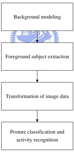
Fig. 1.1 The flowchart of our human activity recognition system. ... 2

Fig. 2.1 The Chromaticity Diagram. ... 8

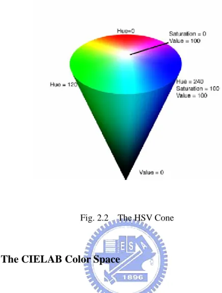
Fig. 2.2 The HSV Cone. ... 10

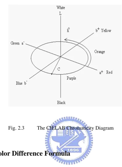
Fig. 2.3 The CIELAB Chromaticity Diagram. ... 12

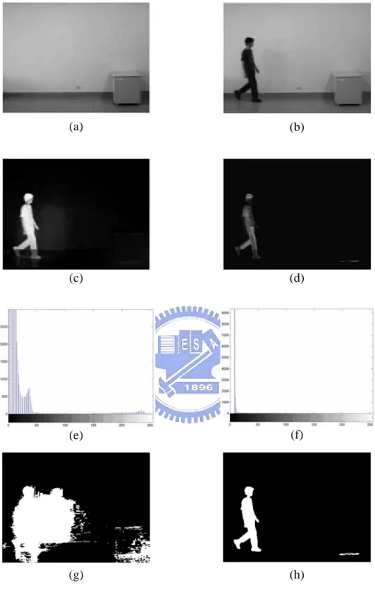
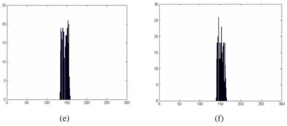
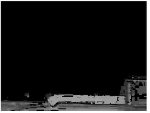
Fig. 3.1 The comparison between frame ratio and frame difference. (a) Background image, (b) image frame with a human, (c) frame difference, (d) frame ratio, (e) histogram of frame difference, (f) histogram of frame ratio, (g) foreground pixels of frame difference after simply taking a threshold, and (h) foreground pixels of frame ratio after simply taking a threshold ... 17

Fig. 3.2 The framework we apply to foreground subject extraction. ... 21

Fig. 3.3 Histogram of binary image projection in X and Y direction... 24

Fig. 3.4 The binary image of extracted foreground region... 24

Fig. 4.1 The experimental environment.. ... 29

Fig. 4.2 Various images of our models. ... 30

Fig. 4.3 Background image. (a) Background image in the H components, (b) Background image in the S components. (c) Background image in the V components.. ... 31

Fig. 4.4 H, S, and V variations versus frame index of background video from frame 1 to frame 300. (a) H at (10, 10), (b) H at (120, 160), (c) S at (10, 10), (d) S at (10, 10), (e) V at (10, 10), and (f) V at (10, 10)... ... 32

Fig. 4.7 An example of foreground extraction at different k thresholds.(a) An image V

frame with subject’s clothing color different from the background, (b) － (f) foreground detected images, (b) kV =1.0, (c) kV =1.1, (d) kV =1.2, (e) kV =1.3,

and (f) kV =1.4... 35 Fig. 4.8 An example of foreground region extraction at different k threshold.(a) An image V

frame with subject’s clothing color similar to the background, (b)－(f) foreground detected images, (b) kV =1.0, (c) kV =1.1, (d) kV =1.2, (e) kV =1.3, and (f)

1.4

V

k = ... 36 Fig. 4.9 The example of the shadow detection. ...37

Fig. 4.10 Foreground detection without and with color compensation. (a)−(c) is the input images, (a1)−(c1) the foreground images, without color compensation, (a2)−(c2) the foreground images detected with color compensation to the whole image. (a3)−(c3) the foreground images detected with color compensation to only foreground subject region...40

Fig. 4.11 The histogram of color difference of the foreground subject. (a) the clothing color is light pink, (b) the clothing color is light yellow and (c) the clothing color is light blue.. ...41

Fig. 4.12 An example of foreground extraction at different k thresholds.(a) An image frame with subject’s clothing color different from the background, (b)−(f) foreground detected images, (b) k = 1, (c) k = 2, (d) k = 3, (e) k = 4, and (f) k = 5...42

Fig. 4.13 An example of foreground extraction at different k thresholds.(a) An image frame with subject’s clothing color similar to the background, (b)−(f) foreground detected images, (b) k = 1, (c) k = 2, (d) k = 3, (e) k = 4, and (f) k = 5.. ...43

Fig. 4.12 The result of the foreground subject extraction in the HSV and CIELAB color space. (a)−(e) is the input images, (a1)−(e1) the foreground images detected in the HSV color space, (a2)−(e2) the foreground images detected in the CIELAB color space... ...45

List of Tables

TABLE I COMPARISON RESULT OF THE PIXEL ACCURACY RATES OVER 300 IMAGES IN

METRIC1 ...47

TABLE II THECOMBINATIONACCURACYRATES INMETRIC1...47

TABLE III COMPARISON RESULT OF THE PIXEL ACCURACY RATES OVER 300 IMAGES IN

METRIC2...48

Chapter 1 Introduction

1.1 Motivation

Human activity recognition from video streams has many applications such as home care system, human-machine interface, and automatic surveillance, etc. However, there is no rigid syntax and well-defined structure in human action recognition system. Therefore, it makes human activity recognition a very challenging task.

Several human activity recognition methods have been proposed in the past few years. Yamato et al. [1] turn image frames into a symbol sequence and use HMM to recognize human action. Bobick and Davis [2] recognize human activities by comparing motion-energy and motion-history of template images with temporal images. Cohen and Li [3] use a view-independent 3-D shape description for classifying and identifying human activity using SVMs. There have been some significant projects on detecting, tracking people and recognizing their activities. W4 [4] is one of them. W4 can detect people (single person or people in group) by adopting an adaptive background model and identify the activities by finding the body parts on the silhouette boundary.

In vision-based systems, foreground subject extraction is usually the first an important step, which is also the objective of this thesis. If we can improve the accuracy of extracting foreground object, then monolithic performance of surveillance

proposed system can be separated into four components. The first component is the background modeling. The second component is the foreground subject extraction. The third component is the transformation of image data into a space which is smaller and easier for posture recognition. The fourth component is the posture classification of an image frame and activity recognition using frame sequences. In this thesis, we emphasize the first two components to improve the accuracy of extracting the foreground image, so that we can enhance the performance of an activity surveillance system.

Fig. 1.1 The flowchart of our human activity recognition system. Background modeling

Foreground subject extraction

Transformation of image data

Posture classification and activity recognition

1.2 Background Modeling

Background subtraction is widely used for detecting moving objects from image frames of static cameras. Most of this work has been based on background subtraction using color or luminance component. In these approaches, difference between the coming frame and the background image is performed to detect foreground objects. W4 [4] is a famous one to be noted. It records the maximum and minimum luminance and the maximum inter-frame difference in every position of a frame in a background video. Then every pixel of the image frame subtracts the maximum and minimum luminance at this position. If the pixel’s absolute value of this difference is larger than the maximum inter-frame difference, the pixel is a foreground.

Background subtraction is extremely sensitive to dynamic scene changes due to illumination change. In order to solve the artifact causing from varying luminance, we develop a method which is more robust to the illumination changes. To this end the method makes use of frame ratio rather than frame difference in the luminance component.

If we utilize only the luminance to do background subtraction, we cannot detect a foreground pixel correctly when the colors of foreground and background are similar. To make fully use of the spectrum of a pixel, it is imperative to do the segmentation in the color domain. In our system, we build our background model in the HSV color space. We use both the luminance and the chromatic components in the background

According to our investigation, we have found that CIELAB color space is developed to become more sensitive in color difference, which also bears the attributes from Hue, Saturation and Lightness. In the CIELAB space, the color difference formula is proposed in this thesis to effectively differentiate the color difference between two colors, where effectiveness becomes significant for close color. The background model records the maximum color difference in every position of an inter-frame in a background video. If the pixel’s color difference between the background and the foreground is lager than a preset maximum color difference, the pixel belongs to the foreground. In this way, the color difference between the background and the foreground becomes larger, and thus the effectiveness of foreground object extraction can be raised greatly.

1.3 Foreground Subject Extraction

Foreground subject extraction is an important step of the vision-based human activity recognition system. Many authors have developed methods of detecting people in images. Park and Aggarwal subtracted foreground pixels from background by computing Mahalanobis distance in each pixel in the HSV color model [5]. Leung and Yang built a human body outline labeling system [6]. Jabri and Duric [7] used color and edge information to improve the quality and reliability of the results. They have all tried to find out the real poses a human did by human body outline or by silhouettes.

Furthermore, the moving cast shadows mostly exhibit a challenge for accurate foreground subject detection. A lot of attempts have been developed to tackle the shadow suppression [8]−[13]encountered in background subtraction. Horprasert et al.

[8] and Cucchiara et al. [9] utilized the rationale that shadows have similar chromaticity, but lower brightness than the background model. Under the proposed frame work in the HSV and color space, we can effectively identify the shadow existence in our detected foreground subject.

After building background models in HSV and CIELAB color spaces, we can extract foreground subjects from video frames by subtracting pixel’s color difference existing in the image frames.

1.4 Thesis Outlines

The thesis is organized as follows. Before introducing the technique of our human activity recognition system, the basic concepts concerning the color difference formula in HSV and CIELAB color spaces are introduced in Chapter 2. In this chapter, we first introduce the HSV and CIELAB color spaces, and then some color difference formulae. Chapter 3 describes in detail our CIELAB-based method, embedded in difference formulae, to build a statistical background modeling for foreground subject extraction. In Chapter 4, the experiment results of the foreground object extraction in the HSV and CIELAB color spaces are shown and compared. At last, we conclude this thesis with a discussion in Chapter 5.

Chapter 2 Introduction to Color Space

In this chapter, we briefly explain the basic concepts of color difference formula, CIELAB and HSV color space.

2.1 The XYZ Color System

The characteristics generally used to distinguish one color from another are, brightness, hue, and saturation.Brightness embodies the chromatic notion of intensity. Hue is an attribute associated with the dominant wavelength in a mixture of light waves. Hue represent dominant color as perceived by observer. Thus, when we call an object red, orange, or yellow, we are specifying its hue. Saturation refers to the relative purity or the amount of white light mixed with a hue. The pure spectrum colors are fully saturated. Colors such as pink (red and white) and lavender (violet and white) are less saturated, with the degree of saturation being inversely proportional to the amount of white light added.

Hue and saturation taken together are called chromaticity, and, therefore, a color may be characterized by its brightness and chromaticity. The amounts of red, green, and blue needed to form any particular color are called the tristimulus values and are denoted, X, Y, and Z, respectively. A color is then specified by its trichromatic coefficients, defined as

x X X Y Z

=

Z Y X Y y + + = (2) and Z Y X Z z + + = (3)

It is noted from these equation that

x+ + = y z 1. (4) For any wavelength of light in the visible spectrum, the tristimulus values needed to produce the color corresponding to that wavelength can be obtained directly from curves or tables that have been compiled from extensive experimental result.

Another approach for specifying colors is to use CIE chromaticity diagram (Fig. 2.1), which shows color composition as a function of x (red) and y (green). For any value of x and y, the corresponding value of z (blue) is obtained form Eq. (4) by noting that z = 1 – (x + y). The point marked green in Fig. 1, for example, has approximately 62% green and 25% red content. From Eq. (4), the composition of blue is approximately 13%

Fig. 2.1 The chromaticity diagram.

The chromaticity diagram is useful for color mixing because a straight-line segment joining any two points in the diagram defines all the different color variations that can be obtained by combining these two colors additively. Consider, for example, a straight line drawn from the red to the green points shown in Fig. 2.1. If there is more red light than green light, the exact point representing the new color will be on the line segment, but it will be closer to the red point than to the green point. Similarly, a line drawn from the point of equal energy to any point on the boundary of the chart will define all the shades of that particular spectrum color.

Extension of this procedure to three colors is straightforward. To determine the range of colors that can be obtained from any three given colors in the chromaticity

diagram, we simply draw connecting lines to each of the three color points. The result is a triangle, and any color inside the triangle can be produced by various combinations of the three initial colors. A triangle with vertices at any three fixed colors cannot enclose the entire color region in Fig. 2.1. This observation supports graphically the remark made earlier that not all colors can be obtained with three single, fixed primaries.

2.2 The Color Space

2.2.1 The HSV Color Space

The HSV (hue, saturation and value) color space corresponds closely to the human perception of color. Conceptually, the HSV color space is a cone. Viewed from the circular side of the cone, the hues are represented by the angle of each color in the cone relative to the 0o line, which is traditionally assigned to be red. The saturation is represent as the distance from the center of the circle. Highly saturation color are on the outer edge of the cone, whereas gray tones (which have no saturation) are at the very center. The brightness is determined by the colors vertical position in the cone. At the point end of the cone, there is no brightness, so all colors are blacks. At the fat end of the cone are the brightness colors.

Fig. 2.2 The HSV Cone

2.2.2 The CIELAB Color Space

The effectiveness of the transformations examined in this section is judged ultimately in print. Since these transformations are developed, refined, and evaluated on monitors, it is necessary to maintain a high degree of color consistency between the monitors used and the eventual output devices. In fact, the colors of the monitors should represent accurately any digitally scanned source images, as well as the final printed output. This is best accomplished with a device-independent color model that relates the color gamut of the monitors and output devices, as well as any other device being used, to one another. The success of this approach is a function of the quality of the color profiles used to map each device to the model and the model itself. The model of choice for many color management systems (CMS) is the CIE L∗a∗b∗

following equations: 116 16 w Y L h Y ∗ _{= ⋅} ⎛ ⎞ ₋ ⎜ ⎟ ⎝ ⎠ (5) 500 W w X Y a h h X Y ∗ ₌ ⎡ ⎛ ⎞₋ ⎛ ⎞⎤ ⎢ ⎜ ⎟ ⎜ ⎟⎥ ⎢ ⎝ ⎠ ⎝ ⎠⎥ ⎣ ⎦ (6) 200 W W Y Z b h h Y Z ∗ ₌ ⎡ ⎛ ⎞₋ ⎛ ⎞⎤ ⎢ ⎜ ⎟ ⎜ ⎟⎥ ⎢ ⎝ ⎠ ⎝ ⎠⎥ ⎣ ⎦ (7) where

( )

⎪⎩ ⎪ ⎨ ⎧ ≤ + ≥ = 0.008856 , 116 / 16 787 . 7 0.008856 , 3 q q q q q h (8)

and X , _W Y , and_W Z are reference white tristimulus values—typically the white of _W

a perfectly reflecting diffuser under CIE standard D65 illumination (defined by x = 0.3127 and y = 0.3290 in the CIE chromaticity diagram of Fig. 2.1 ). The L∗a∗b∗

color space is colorimetric (i.e., color perceived as matching are encoded identically),

perceptually uniform (i.e., color differences among various hues are perceived

uniformly), and device independent. While not a directly displayable format (conversion to another color space is required), its gamut encompasses the entire visible spectrum and can represent accurately the colors of any display, print, or input device. Like the HSI system, the L∗a∗b∗ system is an excellent decoupler of

Fig. 2.3 The CIELAB Chromaticity Diagram

2.3 Color Difference Formula

Based on color difference formula in [14], the CIELAB system is a simplified mathematical approximation to a uniform color space composed of perceived color differences. The perceived lightness L of a standard observer is assumed to follow ∗

the intensity of a color stimulus according to a cubic root law [15]. The colors of lightness L are arranged between the opponent colors green-red and blue-yellow ∗

along the rectangular coordinates a and ∗ b . The total difference between the two ∗

colors is given in terms of L , ∗ a , ∗ b by the CIE 1976 formula ∗

Any color represented in the rectangular coordinate system of axes L , ∗ a , ∗ b can ∗

alternatively be expressed in terms of polar coordinates with the perceived lightness

∗

L and the psychometric correlates of chroma,

C_ab∗ =

( ) ( )

a∗ 2 + b∗ 2 (10) and hue angle,

1 tan . ab b h a ∗ − ∗ ⎛ ⎞ = _{⎜ ⎟} ⎝ ⎠ (11)

In fact, the CIELAB space is not really uniform. If MacAdam or Brown-MacAdam ellipses or ellipsoids are transformed into CIELAB coordinates, differences appear among their axes of up to 1:6.

In particular, at high values of chroma, the simple CIE 1976 color difference formulas value color differences too strongly compared to experimental results of color perception [16]. An improved color difference formula was therefore recommended in 1994 [17]-[19]: 2 2 2 94 , ab ab L L C C H H C H L E k S k S k S ∗ ∗ ∗ ∗ ⎛ Δ ⎞ ⎛Δ ⎞ ⎛Δ ⎞ Δ = _{⎜ ⎟} + _{⎜ ⎟} + _{⎜ ⎟} ⎝ ⎠ ⎝ ⎠ ⎝ ⎠ (12) where ΔL , ∗ ΔCab∗ , and ∗

ΔHab are the CIELAB 1976 color differences of lightness,

chroma, and hue; k , L k , and C kH are factors to match the perception of

[18], [19] have been assumed for the calculations of ΔE94∗ : k_L = k_C = k_H = 1 (13) S_L = 1 (14) 1 0.045 C ab S = + C∗ (15) 1 0.015 . H ab S = + C∗ (16)

Chapter 3 Background Modeling in HSV and

CIELAB Color Space

3.1 Object Extraction in HSV Color Space

3.1.1 The Intensity of the Image

We assume the intensity of the image captured by a camera can be described as

( , ) ( , ) ( , ),

i i i

I x y =S x y r x y (17)

where Ii is the intensity of the image, Si is the spatial distribution of source

illumination, ri is the distribution of scene reflectance, (x,y) is the location of a pixel

in the image, and i is the image sequence index. Now we can compare the difference caused by illumination change between frame difference and frame ratio. If we hold the camera still with no foreground subjects pass by, the reflectance of this background should be the same at any time. That is,

(

,

) (

,

)

. i

r x y =r x y (18)

Although the reflectance is not changed, the effect of illumination is still going on. The frame difference and frame ratio between two consecutive frames can respectively be written as

(

)

( )

(

(

) (

) (

)

)

(

)

(

)

(

)

(

)

(

(

)

)

1 1 1 1 , , , log log , , , , log , log , log , , r r i i r r i i r i r i r r i i I x y S x y r x y I x y S x y r x y S x y S x y S x y S x y − − − − ⎛ ⎞ ⎛ ⎞ = ⎜ ⎟ ⎜ ⎟ ⎜ ⎟ ⎜ ⎟ ⎝ ⎠ ⎝ ⎠ ⎛ ⎞ = ⎜_⎜ ⎟_⎟ ⎝ ⎠ = − (20)

where Id is the intensity of scene captured by camera of frame difference, Sd is the spatial distribution of source illumination of frame difference, and Ir and Sr is of frame ratio. Comparing Eqs. (19) and (20), we can find that the problems cause by reflectance still remains in the frame difference approach; nevertheless, the influence of reflectance is eliminated in the frame ratio approach.

Fig.3.1shows a comparison between frame ratio and frame difference. Fig.3.1(a) is a background image and Fig. 3.1(b) is an image frame with a human. By using frame difference and frame ratio approach, we obtain Fig. 3.1(c) and Fig. 3.1(d), respectively. Gray level of the resulting images distributed from 0 to 255. Fig. 3.1(e) is the histogram of Fig. 3.1(c) and Fig. 3.1(f) is the histogram of Fig. 3.1(d). Comparing the histograms of Fig. 3.1(d) and Fig. 3.1(e), we find out that there was less noise in the region of low gray level by using frame ratio method. The Fig. 3.1(g) and Fig. 3.1(h) are the binary image of extraction images which simply took a threshold value 15 at gray level against Fig. 3.1(c) and Fig. 3.1(d).

(a) (b)

(c) (d)

(e) (f)

(g) (h)

Fig. 3.1 The comparison between frame ratio and frame difference. (a) Background image, (b) image frame with a human, (c) frame difference, (d) frame ratio, (e)

3.1.2 Background Model

If we only use the luminance component to do background subtraction, we cannot detect reliably those foreground pixel whose luminance component close to background pixel. In order to solve this problem, we build our background model in the HSV color space. The HSV color space corresponds closely to the human perception of color. We can have the luminance information and the chromatic information simultaneously.

The hue parameter is the value which represents color information without brightness. Therefore, the hue is not affected by change of the illumination brightness and direction. Although hue is the most useful attribute, there are three problems in using hue attribute for color segmentation: (1) hue is meaningless when the intensity value is very low; (2) hue is unstable when the saturation is very low; and (3) saturation is meaningless when the intensity value is very low [11]. Accordingly, Ohba et al. [20] use three criteria (intensity value, saturation, and hue) to obtain the hue value reliably.

z Intensity Threshold Value:

If V < , then V_t H =0, where V , V , and _t H are an intensity value, the

intensity threshold value, and a hue value, respectively. If measured color is not bright enough, the color is discarded. Then, the hue value is set to a predetermined value, i.e., 0.

z Saturation Threshold Value:

If S< , then S_t H =0, where S , S , and _t H are an saturation value, the

saturation threshold value, and a hue value, respectively. Using this equation, measured color close to gray is discarded in the image.

z Hue Threshold Value:

If H < Δ or P_t H −2π < ΔP_t, then H =0. The range of hue value is from 0 to 2π, and it has discontinuity at 0 and 2π, We use the phase threshold value Δ to avoid the discontinuity effect. P_t

From the result of the previous section, it is advantageous to use frame ratio approach in countering the luminance change. Hence, we propose to utilize the frame ratio to build the background model in the luminance component. We build our background model with the minimum value ( [nH( , ),x y nS( , ),x y nV( , )]x y ) and maximum value ([mH( , ),x y mS( , ),x y mV( , )]x y ) in each HSV domain. Besides, we

also record the inter-frame ratio in the brightness information and the inter-frame different in the chromatic information.

We need a background video, without any moving objects, for background model training. Suppose the observed image frame sequence contains N consecutive images.

( )

, H i

I x y be the pixel’s hue value at

( )

x,y of the i-th image frame. I_iS

( )

x y, be the pixel’s saturation value at

( )

x,y of the i-th image frame. I_iV

( )

x y, be the pixel’s brightness value at

( )

x,y of the i-th image frame. The background model of a pixel is obtained by

( )

( )

( )

( )

{

}

( )

{

}

( )

( )

{

1

}

max , , , min , , max , , H H i i H H i i H H H i i i I x y m x y n x y I x y d x y I x y I₋ x y ⎡ ⎤ ⎡ ⎤ ⎢ ⎥ ⎢ ⎥ ⎢₌ ⎥ ⎢ ⎥ ⎢ ⎥ ⎢ ⎥ ⎢ ⎥ ⎣ ⎦ _{⎢ − ⎥} ⎣ ⎦ ( 21)

( )

( )

( )

( )

{

}

( )

{

}

( )

( )

{

1

}

max , , , min , , max , , S S i i S S i i S S S i i i I x y m x y n x y I x y d x y I x y I₋ x y ⎡ ⎤ ⎡ ⎤ ⎢ ⎥ ⎢ ⎥ ⎢₌ ⎥ ⎢ ⎥ ⎢ ⎥ ⎢ ⎥ ⎢ ⎥ ⎣ ⎦ _{⎢ − ⎥} ⎣ ⎦ (22)

( )

( )

( )

( )

{

}

( )

{

}

( )

( )

{

}

( )

( )

( )

{

}

( )

{

}

( )

( )

{

}

1 1 1 max , min , if , , 1 , _{max , ,} , max , , min , otherwise max , , V i i V V V i i i i V V V i i i V V V i i V i i V V i i i I x y I x y I x y I x y m x y _{I x y I x y} n x y I x y d x y I x y I x y I x y − − − ⎧ ⎡ ⎤ ⎪ ⎢ ⎥ ⎪ ⎢ ⎥ _≥ ⎪ ⎢ ⎥ ⎪ ⎢ ⎥ ⎡ ⎤ ⎪ ⎢ ⎥ ⎢ ⎥ ⎪ ⎣_{= ⎨} ⎦ ⎢ ⎥ _{⎡ ⎤} ⎪ ⎢ ⎥ _{⎢ ⎥} ⎣ _{⎦ ⎪} ⎢ ⎥ ⎪ ⎢ ⎥ ⎪ ⎢ ⎥ ⎪ ⎢ ⎥ ⎪ ⎣ ⎦ ⎩ (23) 1, 2,..., . i= N

3.1.3 Foreground Subject Extraction and Shadow Suppression

Fig.3.2 shows the framework we apply to foreground subject extraction. Our framework of foreground subject extraction is composed of four components. The first component is foreground subject extraction by luminance. The second component is the shadow suppression. The third component is the object segmentation. And the finally component is the color compensation to recover the foreground pixels wrongly classified to the background due to their high luminance similarly.

Fig.3.2 The framework we apply to foreground subject extraction

A. Foreground Subject Detection by Luminance

Foreground objects can be segmented from every frame of the video stream. Each pixel of the video frame is classified to either a background or a foreground

Image

Foreground Subject Detection by Luminance

Shadow Suppression

Object Segmentation

Color Compensation

maximum inter-frame luminance ratio dV

(

x y,

)

of the training background model to segment the foreground pixel by

0, if ( , ) ( , ) ( , ) or ( , ) ( , ) ( , ) ( , ) 255, otherwise V V V i V V V V i V I x y m x y k d x y I x y n x y k d x y B x y ⎧ < ⎪ < ⎪ = ⎨ ⎪ ⎪⎩ (24)

where I_iV

(

x y,

)

is the intensity of a pixel which is located at

( )

x,y , B

( )

x,y is the gray level of a pixel in a binary image, and k is a threshold, determined by light _V

sufficiency of the scene. The value of k is normally set to 1.3 for normal light _V

condition, and k will be reduced for in-sufficient light condition and increased _V

otherwise.

B. Shadow Suppression

The pixels of the moving cast shadows are easily detected as the foreground pixel in normal condition. Because the shadow pixels and the object pixels share two important visual features: motion model and detectability. For this reason, the moving shadows cause object merging and object shape distortion. Horprasert et al. [8] and Cucchiara et al. [9] utilize the rationale that shadows have similar chromaticity, but lower brightness than the background model. Hence, we can detect the shadow from foreground subject in the HSV color space. We analyze only points belonging to possible moving object that are detected in step A. We define a shadow mask S for each ( , )x y point as follows:

shadow, if ( , ) ( , ) 0 and ( , ) ( , ) (x,y) ( , ) _{and ( , ) ( , ) (x,y)} object, V V i H H H i H S S S i S I x y n x y I x y m x y k d S x y _{I x y m x y k d} − < − < = _{− <} otherwise ⎧ ⎪ ⎪ ⎪ ⎨ ⎪ ⎪ ⎪ ⎩

whereIiH( , )x y ,IiS( , )x y , and IiV

(

x y,

)

are respectively the HSV channel of a pixel

located at

( )

x,y , and S x y

(

,

)

is the shadow mask to class the pixel in the moving cast shadow. Values k and S k are selected threshold values used to measure the H

similarities of the hue and saturation between the background image and the current observed image. We can utilize the shadow mask ( , )S x y to change the shadow

pixels into background in B x y . ( , )

C. Object Segmentation

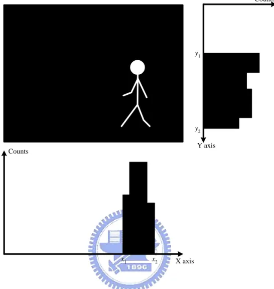
According to the binary image B segmented by above, we extract the region of foreground object to minimize the image size. Foreground region extraction can be accomplished by simply introducing a threshold on the histograms in X and Y direction. Fig. 3.3 shows an example of foreground region extraction. We utilize the binary image and project it to X and Y directions. The interested section has higher counts in the histogram. We obtain the boundary coordinates x1, x2 of X axis and y1, y2

of Y axis from the projection histogram. We can use these boundary coordinates as the corner of a rectangle to extract foreground region (B ). Fig. 3.4 is the extracted s

foreground region.

X axis Counts Counts Y axis x₁ x₂ y₁ y₂

Fig. 3.3 Histogram of binary image projection in X and Y direction.

D. Color Compensation

Some colors such as yellow, pink, and light blue have similar luminance value. If we only use the luminance component to do background subtraction, we cannot detect foreground pixel correctly when its luminance is similar to that of a background pixel. In order to improve detectability, background subtraction is computed by taking into account not only a point’s luminance, but also its chromaticity. We want to use the chromaticity to enhance the accuracy of the foreground object. We only analyze the region B obtained in subsection C above. Based on the amount of the chromaticity s

change, we reanalyze its background in B to be changed to a foreground of object, s

by 255, if ( , ) ( , ) (x,y) or ( , ) ( , ) (x,y) ( , ) 0, otherwise S S S i S H H H i H f I x y m x y k d I x y m x y k d B x y ⎧ − > ⎪ ⎪ − > = ⎨ ⎪ ⎪ ⎩

where IiH( , )x y andIiS( , )x y are respectively the hue and saturation components of a

pixel at

( )

x,y , k and S kH are selected threshold values. B is the final f

foreground object after the refined step ofEq. (26).

3.2 Object extraction in CIELAB color space

3.2.1 Background Model

According to CIELAB’s sensitiveness on color difference, we can have subtle color difference measure in the CIELAB color space, which also bears the attributes of Hue, Saturation and Lightness. In order to compute the genuine difference between two colors and thus raise the sensitivity of foreground object extraction by a larger color difference between the background and the foreground, we build a statistical background model by in CIELAB color space combined with color difference formula.

We need a background video, without any moving objects, for background model training. Suppose the observed image frame sequence contains N consecutive images. First of all, we have to do the color separation on the N consecutive images of background video.

We can obtain the tristimulus values of X, Y and Z from the values of R, G and B by linear transform on the N consecutive images as follows:

⎥ ⎥ ⎥ ⎦ ⎤ ⎢ ⎢ ⎢ ⎣ ⎡ ⎥ ⎥ ⎥ ⎦ ⎤ ⎢ ⎢ ⎢ ⎣ ⎡ = ⎥ ⎥ ⎥ ⎦ ⎤ ⎢ ⎢ ⎢ ⎣ ⎡ B G R Z Y X 939 . 0 130 . 0 020 . 0 071 . 0 707 . 0 222 . 0 178 . 0 342 . 0 431 . 0 (27)

However, the tristimulus values X, Y and Z are transformed into chromaticity coordinate, the homogenization of this color space is not good. Therefore, the color difference calculated by color difference formula in X, Y and Z domain can not factually represent the color difference between the two colors. In order to resolve the

problem of the homogenization in the color domain, we transform the tristimulus values into CIELAB color space from the X, Y and Z domain on the N consecutive images, and we can find the color difference between two colors, especially for two very similar colors. In the CIELAB color space, background modeling can become more sensitive and hence more effective in foreground subject extraction.

In CIELAB space, we calculate the arithmetic mean from these N consecutive images to represent the background, and find the maximum color difference in every pixel of an inter-frame among the background image by.

, ) , ( 1 ) , ( 1

∑

= = N i i L L x y N y x m (28) , ) , ( 1 ) , ( 1

∑

= = N i i a a x y N y x m (29) , ) , ( 1 ) , ( 1

∑

= = N i i b b x y N y x m (30)

where ),m_L(x, y m_a(x, y) and m_b(x, y) are respectively the L, a and b components of the arithmetic mean of a pixel at (x , y) of these N images.

The background model of a pixel is obtained by

{

b

}

1 ( , ) max _a ( , ) , N d x y E x y − = Δ (31)

where ΔE_ab (x, y) is the color difference at (x, y), in Eq. (9) of Chapter2, of the background images.

3.2.2 Foreground Subject Extraction

Foreground objects can be segmented from every frame of the video stream. Each pixel of the video frame is classified to either a background or a foreground pixel by the difference between the background model and a captured image frame. We utilize the maximum inter-frame color difference d(x, y) of the training background model to segment the foreground pixel by

(

)

⎪ ⎪ ⎩ ⎪⎪ ⎨ ⎧ > Δ = ) , ( ) , ( if , 255 otherwise , 0 , y x d k y x E y x B i ab (32) where

(

) (

2

) (

2

)

2 ( , ) ( , ) ( , ) ( , ) , i i i i ab E x y L x y a x y b x y Δ = Δ + Δ + Δ (33) and ( , ) ( , ) ( , ) , i i L L x y L x y x y Δ = − m (34) ( , ) ( , ) ( , ) , i i a a x y a x y x y Δ = − m (35) ( , ) ( , ) ( , ) . i i b b x y b x y x y Δ = − m (36)

Therefore, B

( )

x,y is the resulting binary image after segmentation. In the above equation, k is a threshold, determined by light sufficiency of the scene. The value of k is normally set to 2 for normal light condition, and k will be reduced for in-sufficient light condition and increased for sufficient lighting.

Chapter 4

Experimental Result

In our experiment, we tested our system on videos taken by digital camera. We took the video in our laboratory at the 5th Engineering Building in NCTU campus. The camera has a frame rate of thirty frames per second and image resolution is

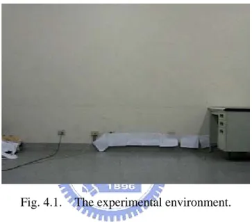
320 240× pixels. The experimental environment is shown in Fig. 4.1.

Fig. 4.1. The experimental environment.

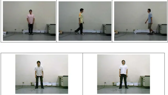
The background is not complex and we equipped a table in the scene. The light source is fluorescent lamps and is stable. The models clothing color are“pink,＂ “ yellow, ＂ “ light blue, ＂ “ ivory, ＂ and “ white. ＂ We test the foreground detection capability depending on the light color clothing worn by action subjects, and the similarity of the colors of subject’s clothing and background. When the colors of clothing and background are similar, a moving object, such as human body, may not be segmented easily from image frame. We compare the detection result in the HSV and CIELAB space. Fig. 4.2 shows our models in the experiment.

Fig. 4.2. Various images of our models.

4.1 Background Model Construction

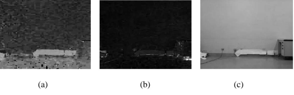
We built the background model in the HSV and CIELAB color space. The value of H or S or V is between 0 and 255. Figs. 4.3(a), 4.3(b), and 4.3(c) show the background image in the H, S, and V component, respectively. We can find from these three figures that the hue value is relatively unstable when the saturation is close to zero. We make an experiment to test the changes in the HSV components in constructing the background model. Fig. 4.4 represents the H, S, and V variations of two pixels at coordinates ( , )x y = (10, 10) and ( , )x y = (120, 160) during the first 300

frames in the background video. From Fig. 4.4, we can see that V component is most stable of the background model. H and S components are less stable than V. Hence, we need to solve this problem.

(a) (b) (c)

Fig. 4.3. Background images. (a) Background image in the H component, (b) Background image in the S component, and (c) Background image in the V component.

(e) (f)

Fig. 4.4. H, S, and V variations versus frame index of background video from frame 1 to frame 300. (a) H at (10, 10), (b) H at (120, 160), (c) S at (10, 10), (d) S at (10, 10), (e) V at (10, 10), and (f) V at (10, 10).

In Sec. 3.1.2, we know that hue is unreliable when the color is close to the gray tones. Hence, we use three criteria (V S Ht, t, t) to obtain the hue value reliably in

building the background model. In our experiment, we set three criteria by

50, 50, and 25

t t t

V = S = H =

to make hue value reliably.

Fig. 4.5 shows the background image in the H color components after we use above criterion to redefine it. We can find that the hue values in the background image are almost be set to zero. The reason is that our background is simple and the color is similar to the gray tones.

Fig. 4.5. Background image in the redefined H color components.

The background model in the CIELAB color space records the maximum color difference in every position of an inter-frame in 100 out of 300 background image frames. Fig. 4.6 shows the histogram of background training.

4.2

Foreground Subjects Extraction

4.2.1 Foreground Detection in HSV Color Space

In segmenting the images, the V color component is usually stable and reliable, but it has two drawbacks: the V component is insensitive to the similar, especially lighting, color such as yellow, pink, and light blue. When the subjects wear the clothing with the color different from the background, we can do background subtraction well in the V color component.

In the first step, we use the frame ration in the V color component to get the binary image B x y in Eq. (24) described in Sec. 3.1.3. The value ( , ) k is chosen by V

experiments and varies with different trials. Hence, we ran a series of experiments to determine the optimal threshold k When the subject’s clothing color different from V. the background, Fig. 4.7 shows the binary image ( , )B x y obtained by different

. V

k s＇ When subject’s clothing color similar to the background, Fig. 4.8 shows the binary image B x y obtained by different( , ) k sV＇. Comparing Figs. 4.7 and 4.8, we

can find that if the color is different from the background, we can use the threshold value k to get a good foreground subject extraction. But we cannot adjust V k to V

get a complete and noise-free foreground subject when the clothing color is similar to the background. After the experiment, we set kV =1.3 in the HSV color system.

(a) (b)

(c) (d)

(e) (f)

Fig. 4.7. An example of foreground extraction at different k thresholds. V

(a) An image frame with subject’s clothing color different from the background, (b)−(f) foreground detected images, (b) kV =1.0, (c) kV =1.1, (d) kV =1.2, (e)

1.3

V

(a) (b)

(c) (d)

(e) (f)

Fig. 4.8. An example of foreground region extraction at different k threshold. V

(a) An image frame with subject’s clothing color similar to the background, (b)−(f) foreground detected images, (b) kV =1.0, (c) kV =1.1, (d) kV =1.2, (e) kV =1.3,

and (f) kV =1.4,

During the foreground extraction, the shadowing effect introduces artifact foreground subjects and deteriorates the recognition result. We use the shadow mask, which including the shadow characteristic existing in HSV domains of Eq. (25) described in Sec. 3.1.4 to classify the pixels whether it is a shadow point or not. Fig.

4.9 shows the process result regarding shadow suppression. Figs. 4.9(a) and (b) are two input images. Figs. 4.9(c) and (d) are the foreground subject without shadow suppression. The foreground subject with shadow suppression is shown in Figs. 4.9(e) and (f), which improves greatly comparing with Figs. 4.9(c) and (d).

(a) (b)

(c) (d)

(e) (f)

The models wear light blue clothing, yellow clothing, and pink clothing, respectively. In the previous experiment, we cannot adjust k to get a complete and V

clean foreground subject. Hence, we do the color compensation in Eq. (26) described in Sec. 3.1.3. In what follows, the effectiveness of color compensation in obtaining a more accurate foreground is described in Fig. 4.10.

From the Figs. 4.10(a2)-(c2), we can find a trade-off between the foreground and the background detection by color compensation step to the whole image. Hence we cannot get a complete and noise-free foreground subject when the clothing color is similar to the background.

From the Figs. 4.10(a3)-(c3), we have found that we can get good compensation when the clothing color is light blue and yellow, but cannot obtain good compensation when the clothing color is pink. The reason is that when pink color pixels are transformed from RGB color space to HSV color space, the saturation of pink is lower than the set criterion S . Hence, we cannot recover those pixels from t

(a) (a1)

(a2) (a3)

(b) (b1)

(c) (c1)

(c2) (c3)

Fig. 4.10. Foreground detection without and with color compensation. (a)−(c) is the input images, (a1)−(c1) the foreground images, without color compensation, (a2)−(c2) the foreground images detected with color compensation to the whole image. (a3)−(c3) the foreground images detected with color compensation to only foreground subject region.

4.2.2 Foreground Detection in CIELAB Color Space

We utilize the maximum inter-frame color difference d(x, y) of the training background model to get the binary image B x y in Eq. (32) described in Sec. 3.2.3, ( , ) and use the “foreground subject ground truths” to record the color difference of foreground pixel simultaneously. Fig. 4.11 shows the histogram of color difference of the foreground subject.

(a) (b) (c)

Fig. 4.11. The histogram of color difference of the foreground subject. (a) the clothing color is light pink, (b) the clothing color is light yellow and (c) the clothing color is light blue.

The value k is chosen by experiments and varies with different trials. Hence, we ran a series of experiments to determine the optimal threshold k. When subject’s clothing color different from the background, Fig. 4.12 shows the binary image

( , )

B x y obtained by different k’s. When subject’s clothing color similar to the

(a) (b)

(c) (d)

(e) (f)

Fig. 4.12. An example of foreground extraction at different k thresholds.(a) An image frame with subject’s clothing color different from the background, (b)−(f) foreground detected images, (b) k = 1, (c) k = 2, (d) k = 3, (e) k = 4, and (f) k = 5

(a) (b)

(c) (d)

(e) (f)

Fig. 4.13. An example of foreground extraction at different k thresholds.(a) An image frame with subject’s clothing color similar to the background, (b)−(f) foreground detected images, (b) k = 1, (c) k = 2, (d) k = 3, (e) k = 4, and (f) k = 5

From Fig. 4.12 and Fig. 4.13, we can find that if the color is different from or similar to the background, we can use the threshold value k to get a good foreground subject extraction in the CIELAB space. In general condition, the suitable range of

4.3

Comparing the Experimental Result

The results of the foreground subject extraction in the HSV and CIELAB color spaces are showed in Fig. 4.14, the left column contains input images; the middle column contains the resulting foreground images detected in the HSV color space; and the right column is the resulting foreground images detected in the CIELAB color space.

(a) (a1) (a2)

(b) (b1) (b2)

(d) (d1) (d2)

(e) (e1) (e2)

Fig. 4.14 The result of the foreground subject extraction in the HSV and CIELAB color space. (a)−(e) is the input images, (a1)−(e1) the foreground images detected in the HSV color space, (a2)−(e2) the foreground images detected in the CIELAB color space.

We selected over 300 frames from the video sequence of the model with a subject wearing clothing similar to the background color. The “foreground subject ground truths” of these 300 frames were generated manually. Let A be a detected foreground subject region and B be the corresponding “ground truth.” Then we test the pixel accuracy by the following two metrics. Metric 1, accuracy rate , is a ₁ measure concerning whole segmented region pixels relative to these pixels in A the same with in B. To this end, we calculate the accuracy rate by

where Ntotal is the pixel number of segmented foreground image, and N is the s

pixel number that the pixel in A is the same as that in B, i.e., such of true positive and false negative pixels of A relative to B. Metric 2, accuracy rate , is adopted from [21] ₂ by 2 Accuracy rate A B 100%. A B ∩ = × ∪ (38)

This measure counts the percentage of the mutual positive pixels to expanded positive pixels. We consider the accuracy rate of the foreground subject and the background in metric 1 and 2. Table I and III show the accuracy rate of the foreground subject and the background in metric 1 and 2 of over 300 frames, and the HSV (i) and (ii) is the accuracy rate of the foreground images detected with color compensation to the whole image and only foreground subject region, respectively. Table II and IV show the combination accuracy rate of the foreground subject combined with the background by linear interpolation, and demonstrate the improvement of the foreground subject extraction in the CIELAB color space over that in the HSV color Space.

TABLE I

COMPARISON RESULT OF THE PIXEL ACCURACY RATES OVER 300IMAGES INMETRIC1

Accuracy rate (%) ₁

HSV (i) HSV (ii) CIELAB

Foreground Background Foreground Background Foreground Background

Pink 58.91 98.86 62.39 99.42 90.55 98.72 Yellow 82.72 96.32 82.06 99.26 90.67 98.64 Light Blue 78.78 95.06 89.82 99.58 92.96 98.67 White 67.33 98.03 71.68 98.91 83.24 99.15 Ivory 58.42 98.31 64.21 99.13 77.55 99.35 TABLE II

THECOMBINATIONACCURACYRATES INMETRIC1

Combination Accuracy rate (%) ₁

HSV (i) HSV (ii) CIELAB

Pink 60.24 64.46 91.02

Yellow 83.5 83.02 91.44

Light Blue 81.41 90.1 93.24

White 69.53 73.72 84.47

TABLE III

COMPARISON RESULT OF THE PIXEL ACCURACY RATES OVER 300IMAGES INMETRIC2 Accuracy rate (%) ₂

HSV (i) HSV (ii) CIELAB

Foreground Background Foreground Background Foreground Background

Pink 48.47 96.42 56.69 97.22 86.41 98.37 Yellow 52.27 95.32 73.09 98.22 85.41 98.15 Light Blue 42.59 93.96 83.14 99.02 87.73 98.35 White 51.32 96.77 63.03 96.69 75.11 97.78 Ivory 49.17 96.01 57.89 96.35 71.67 97.56 TABLE IV

THECOMBINATIONACCURACYRATES INMETRIC2

Combination Accuracy rate (%) ₂

HSV (i) HSV (ii) CIELAB

Pink 51.17 58.97 87.62 Yellow 54.68 74.49 86.12 Light Blue 45.26 83.96 88.28 White 53.02 65.54 76.82 Ivory 41.45 60.76 73.64 Average 49.12 68.74 82.5

Chapter 5

Conclusion

In this thesis, we have proposed the foreground subject extraction in the CIELAB color space. Embedded in CIELAB space, our method exploits color difference formula to raise the sensitivity of color detection. In the CIELAB color space, we still can utilize not only the luminance component but also the chromatic component existent in the background image. In this way, we can reliably extract the foreground subject, even when the foreground chrominance is similar to that of the background. Experimental results have shown of the foreground subject extraction is better in the CIELAB color space than HSV Color space.

In the future study, we can apply our method to human activity recognition system. The recognition rate can be raised owing to better segmentation capability. In addition, utilization other color difference formulae, detection by a camera moving at a fixed velocity, extensions of various test environments, and more complicated surrounding are our future work.

References

[1] J. Yamato, J. Ohya, and K. Ishii, “Recognizing human action in time- sequential images using Hidden Markov model,” In Proc. IEEE CVPR, pp. 379−385, 1992. [2] F. Bobick and J. W. Davis, “The recognition of human movement using temporal

templates,” IEEE Trans. Pattern Anal. Machine Intell., vol. 23, no. 3, 2001. [3] I. Cohen and H. Li, “Inference of human postures by classification of 3D

human body shape,＂ in Proc. IEEE Int. Workshop on Anal. Modeling of Faces

and Gestures, pp. 74−81, 2003.

[4] I. Haritaoglu, D. Harwood, and L. S. Davis, “W4: real-time surveillance of people and their activities,” IEEE Trans. Pattern Anal. Machine Intell., vol. 22, no. 8, pp. 809−830, 2000.

[5] S. Park and J. K. Aggarwal, “Segmentation and tracking of Interacting human body parts under occlusion and shadowing,” in Proc. of the Workshop on Motion

and Video Computing, pp.105−111, 2002.

[6] M. K. Leung and Y. H. Yang, “First sight: A human-body outline labeling system,” IEEE Trans. Pattern Anal. Machine Intell., vol. 17, no. 4, pp. 359−377,1995.

[7] S. Jabri, Z. Duric, H. Wechsler, and A. Rosenfeld, “Detection and location of people in video images using adaptive fusion of color and edge information,” in

Proc. Int. Conf. Pattern Recognition, pp. 627−630, 2000.

[8] T. Horprasert, D. Harwood, and L.S. Davis, “A statistical approach for real-time robust background subtraction and shadow detection,” in Proc. IEEE ICCV’ 99, 1999.

[9] R. Cucchiara, C. Grana, M. Piccardi and A. Prati, “Improving shadow suppression in moving object detection with HSV color information,” in Proc.

IEEE Intelligent transportation System Conference, pp. 334−339, 2001.

[10] A. Prati, I. Mikic, M. Trivedi and R. Cucchiara, “detecting moving shadows:slgorithms and evaluation,” in Proc. IEEE Transactions on Pattern Analysis and Machine Intelligence, vol. 25, no. 7, pp. 918−923, 2003.

[11] B. Chen and Y. Lei, “Indoor and outdoor people detection and shadow suppression by exploiting HSV color information,” in Proc. Fourth Int. Conf. on

Computer and Information Technology, pp. 137−142, 2004.

[12] S. Vitabile, G. Pilato, G. Pollaccia, and F. Sorbello, “Road signs recognition using a dynamic pixel aggregation technique in the HSV color space,” in Proc. 11th Int.

Conf. on Image Analysis and Processing, pp. 572−577, 2002.

[13] R. Cucchiara, M. Piccardi and A. Prati, “Detecting moving objects, ghosts, and shadows in video streams,” IEEE Transactions on Pattern Analysis and Machine

Intelligence, vol. 25, no. 10, pp. 1337−1342, 2003.

[14] B. Hill, Th. Roger, and F. W. Corhagen, “Comparative analysis of the quantization of color space on the basis of the CIELAB color-difference formula,” ACM Transaction on Graphics, vol. 16, no. 2, April 1997, Pages 109-154.

[15] CIE. 1986a. Colorimetry. CIE Pub. 15.2, 2nd ed., Commission International de L’Eclairage, Vienna, 29-30

[16] Loo, M. R. and Rigg, B. 1987 BFD (1:c) colour-difference formula. Part 1: Development of the formula. JSDC 103 (Feb.), 126-132. Part 2: Performance of the formula. JSDC 103 (March), 86-94.

Commission International de L’Eclairage, Vienna.

[19] CIE. 1995. Industrial color-difference evaluation. CIE Pub. 116, Commission International de L’Eclairage, Vienna.

[20] K. Ohba, Y. Sato, and K. Ikeuchi, “Appearance-based visual learning and object recognition with illumination invariance,” Machine Vision and Applications, Vol. 12, No. 4, pp. 189−196, 2000.

[21] L. Li, W. Huang, I. Y. H. Gu, and Q. Tian, “Statistical modeling of complex backgrounds for foreground object detection,” IEEE Transactions of Image