國立交通大學
電子工程學系 電子研究所
碩 士 論 文
適用於
H.264/AVC 分數像素移動估測之快速演
算法與設計
Fast Algorithm and Design for H.264/AVC
Fractional-pel Motion Estimation
研 究 生:郭子筠
指導教授:張添烜 博士
適用於H.264/AVC 分數像素移動估測之快速演算法與設計
Fast Algorithm and Design for H.264/AVC Fractional-pel Motion Estimation
研 究 生:郭子筠
Student:
Tzu-Yun
Kuo
指導教授:張添烜 博士
Advisor:
Dr.
Tian-Sheuan
Chang
國立交通大學
電子工程學系 電子研究所
碩士論文
A Thesis
Submitted to Department of Electronics Engineering & Institute of Electronics College of Electrical & Computer Engineering
National Chiao Tung University in partial Fulfillment of the Requirements
for the Degree of Master
in
Electronics Engineering & Institute of Electronics July 2007
Hsinchu, Taiwan, Republic of China
i
適用於
H.264/AVC 分數像素移動估測之快速演
算法與設計
研究生:郭子筠 指導教授:張添烜博士 國立交通大學 電子工程學系 電子研究所摘要
隨著高解析數位電視時代的來臨,為了兼顧大且精緻的畫面,高壓縮率規格 (H.264/AVC)是我們現行的解決方案。因為在視訊編碼上用了更多的壓縮技巧, 它不僅可有效節省儲存媒體所需的空間,同時也可在現行的通訊環境下允許傳輸 更高解析的畫面。但是伴隨著種種好處而來的,就是尤其在高畫值應用中極之龐 大的運算量。 這篇論文提出了適用於高畫值 H.264/AVC 分素像素移動的快速演算法及其 硬體架構。為了解決高畫值應用中的龐大計算時間,我們提出只搜尋六點的單一 疊代快速演算法。這個單一疊代的演算法利用移動向量預測器來預估可能的分數 移動向量,由此減少了88%的分數位移估測搜尋點數,並且讓分數位移估測的運 算所需要的疊代次數減半;另外我們使用4x4 哈達瑪轉換而非 8x8 哈達瑪轉換來 作為價值函數的計算方式,以減少其運算量和大約75%的轉換裝置面積。拜快速 演算法之賜,分數移動估測部分跟之前的研究相比,其架構可以減少20%的面積 及增進40%的運算處理速度。ii
Fast Algorithm and Design for H.264/AVC
Fractional-pel Motion Estimation
Student : Tzu-Yun Kuo Advisor: Dr. Tian-Sheuan Chang
Department of Electronics Engineering & Institute of Electronics National Chiao Tung University
Abstract
With modern day advances in computer processing and multimedia applications, improvements in the area of image processing and video compression are analogous. Video compression allows the reduction of high-resolution video into a more compact memory space to thereby reduce storage and video processing resources. But the playback is the growth of computational complexity, especially in HD-sized application.
This thesis presents a set of fast algorithm and VLSI architecture for HDTV-sized H.264 fractional motion estimation. To solve the long computational latency in HD-sized application, we propose to use the single iteration algorithm with only six search points. This single iteration method uses the information of motion vector predictor to predict the fractional motion vector and thereby reduces 88% search points and halves the cycle count of two iteration methods in previous approaches. Moreover, we propose to use 4x4 Hadamard instead of 8x8 Hadamard as cost function for H.264 high profiles without significant video quality loss and 75% area reduction of the transform unit. By these techniques, the resulted architecture can save
iii
20% of area and provide over 40% of throughput improvement than the previous work, and is able to support HDTV applications.
iv
誌 謝
首先誠摯的感謝指導教授張添烜博士,老師悉心的教導使我得以一窺 視訊編碼領域的深奧,不時的討論並指點我正確的方向,使我在這些年中 獲益匪淺。老師對學問的嚴謹更是我輩學習的典範。 同時也要謝謝我的口試委員們,交大電子李鎮宜教授和清華電機陳永 昌教授,感謝教授們百忙之中抽空來指導我,各位的寶貴意見讓本論文更 加完備。 兩年裡的日子,實驗室裡共同的生活點滴,學術上的討論、言不及 義的閒扯、讓人又愛又怕的宵夜、趕作業的革命情感、因為睡太晚而遮遮 掩掩閃進實驗室...,感謝眾位學長、同學、學弟的共同砥礪,你們 的陪伴讓兩年的研究生活變得絢麗多彩。 感謝林佑昆、張彥中、鄭朝鐘、古君偉、王裕仁、蔡旻奇、余國亘、 吳錦木、李國龍學長們不厭其煩的指出我研究中的缺失,且總能在我迷惘 時為我解惑,也感謝李得瑋、林嘉俊、吳秈璟、廖英澤同學的幫忙,恭喜 我們順利走過這兩年。實驗室的戴瑋呈、張瑋城、曾宇晟、蔡宗憲、詹景 竹學弟們當然也不能忘記,你們的幫忙及搞笑我銘感在心。 最後,謹以此文獻給我摯愛的雙親。v
Content
Chapter 1 Introduction...1
1.1 MOTIVATION...1
1.2 THESIS ORGANIZAION ...3
Chapter 2 Overview of H.264/AVC Standard ...4
2.1 OVERVIEW ...4
2.1.1 Variable block-size motion compensation with multiple references ....4
2.1.2 Directional spatial intra coding...4
2.1.3 In-loop deblocking filter ...5
2.1.4 Context adaptive entropy coding ...5
2.1.5 Encoding flow...5
2.1.6 Profiles ...6
2.2 INTRA PREDICTION...9
2.3 INTER FRAME PREDICTION ...10
2.4 TRANSFORM ...12
2.5 QUANTIZATION...13
2.6 ENTROPY CODING...13
Chapter 3 Review of FME Search Algorithms...15
3.1 SEARCH ALGORITHM IN THE REFERENCE SOFTWARE [12] ...15
3.1.1 Algorithm ...15
3.1.2 Hardware implementation[16] ...16
3.2 FIVE CANDIDATES ALGORITHM [15] ...17
3.2.1 Algorithm ...17
3.2.2 Hardware implementation...19
3.3 QUADRATIC PREDICTION BASED FME [14]...21
3.4 CENTER-BIASED FRACTIONAL-PEL SEARCH (CBFPS)[13] ...23
3.5 FAST FRACTIONAL-PEL ME AND MODE DECISION[17]...25
3.5.1 Algorithm ...25
3.5.2 Hardware implementation...27
3.6 SUMMARY ...28
Chapter 4 A Single Iteration Fractional-pel Motion Estimation Algorithm ...30
4.1 PROPOSED SINGLE ITERATION ALGORITHM ...30
4.1.1 Proposed SIFME Algorithm ...30
4.1.2 Analysis of prediction accuracy and search point...32
vi
4.2 SIMULATION RESULT & COMPARISON ...36
Chapter 5 Architecture Design for Fast Sub-Pel Motion Estimation...41
5.1 HARDWARE CONSIDERATION...41
5.2 HARDWARE CONSIDERATION FOR FME...42
5.3 ARCHITECTURE ...46
5.3.1 Functional flow and overall architecture ...46
5.3.2 Reference SRAMs ...49
5.3.3 FME luma module ...52
5.3.4 Other modules...56
5.4 IMPLEMENTATION RESULT...61
5.5 PERFORMANCE ANALYSIS...63
Chapter 6 Conclusion ...64
vii
List of Figures
Fig. 1 Block diagram of H.264 encoder...6
Fig. 2 Profiles...8
Fig. 3 (a) Intra_4_4 prediction is conducted for samples a-p of a block using samples A-Q...9
Fig. 4 Inter macroblock partitions...11
Fig. 5 Fractional interpolation for motion compensation ...11
Fig. 6 Multiple reference frame motion compensation...12
Fig. 7 Search algorithm in the reference software ...15
Fig. 8 Five candidates search algorithm ...17
Fig. 9 Refine position in case 1...18
Fig. 10 Refine position in case 2...18
Fig. 11 Refine position in case 3...18
Fig. 12 Refine position in case 4...19
Fig. 13 Block diagram of hardware of 5 candidates algorithm...19
Fig. 14 The integer-pixel search positions within the "local" fractional-pel ME search area...21
Fig. 15 (a) Sub-pel motion vector distribution using the Full Search algorithm versus the (0,0) MV (b) Sub-pel motion vector distribution using the Full Search algorithm versus the median predictor...23
Fig. 16 The integer and half pixels within the fractional-pel ME search area. ...25
Fig. 17 Top-level architecture in [17] ...27
Fig. 18 The proposed SIFME algorithm flow on two square points, (0,0) and frac_pred_mv, and four triangle point around frac_pred_mv in one quarter-pel distance...30
Fig. 19 Rate distortion curve of the four CIF size sequences ...38
Fig. 20 Rate distortion curve of the four 720p size sequences ...39
Fig. 21 Rate distortion curve of the seven 1080p size sequences...39
Fig. 22 The block diagram of proposed H.264 high profile encoder...42
Fig. 23 The mode filtering algorithm of integer pixel motion estimation ...44
Fig. 24 Function flow in FME stage ...46
Fig. 25 Block diagram of FME Top Stage ...48
Fig. 26 Block diagram of Mode0 Reference Pixel SRAM ...49
Fig. 27 Block diagram of Mode1 Reference Pixel SRAM ...50
Fig. 28 Block diagram of Chroma Reference Pixel SRAM...51
viii
Fig. 30 Interpolation unit ...53 Fig. 31 (a) 4X4 block PU (b) 6-tap 1-D FIR filter...54 Fig. 32 Block diagram of FME chroma hardware. It contains 7 registers, 4
PEs and 2 subtracters ...56 Fig. 33 Block diagram of Processing Element(PE) in FME chroma module.
...57 Fig. 34 The relationship of the 7 values in the registers in space domain ...58 Fig. 35 Block diagram of Discrete Cosine Transform(DCT) hardware...59
ix
List of Tables
Table 1 Hit rate of motion vector (mvx and mvy) compared to the algorithm adopted by JM...32 Table 2 Search point comparisons for different algorithms...33 Table 3 Comparisons of number of processing unit(PU) and number of
iterative search steps ...33 Table 4 Simulation results of SIFME with different SATD methods when
compared to the reference software[12] ...35 Table 5 PSNR & bit rate comparison for different 720p sequences and QPs.
Speed up is only the performance in fractional ME part ...37 Table 6 PSNR & bit rate comparison for different 1080p sequences and QP
...37 Table 7 Simulation result when QP = 28, speed up is only the performance
in fractional ME part. RDO is off, reference frame number = 1, 300f, CIF ...40 Table 8 Synthesis result of the fast FME luma architecture in UMC013 ....61 Table 9 Synthesis result of the FME top stage in UMC013 ...62 Table 10 Comparison between the proposed fast FME luma architecture and other architecture ...63
1
Chapter 1 Introduction
With the demand of higher video quality and lower bit rate, a new international video coding standard is developed by the Joint Video Team (JVT) of ISO/IEC MPEG and ITU-T VCEG, which is known as H.264 or MPEG-4 Part 10 Advanced Video Coding (AVC)0. Comparing with MPEG-2 and MPEG-4, H.264/AVC can improve the coding efficiency by up to 50%[2] while still keep the same video quality with various advanced coding tools.
1.1 MOTIVATION
The early video standard, MPEG-1, is aimed at CD-ROM based video storage. Subsequently, the MPEG-2 video coding standard[3], as an extension of prior MPEG-1 standard[4], supports the application such as the transmission of standard definition(SD) and high definition(HD) TV signals over satellite, cable, and terrestrial emission and the storage of high-quality SD video signals onto DVDs. Recently the MPEG-4 standard[5] also emerges in some application domains of the prior coding standards.
In 2001, the ISO Motion Picture Experts Group (MPEG) recognized the potential benefits of H.26L and the Joint Video Team (JVT) was formed, including experts from MPEG and VCEG. JVT’s main task is to develop the draft H.26L “model” into a full International Standard. In fact, the outcome will be two identical standards: ISO MPEG4 Part 10 of MPEG4 and ITU-T H.264. The “official” title of the new standard
2
is Advanced Video Coding(AVC); however, it is widely known by its old working title, H.26L and by its ITU document number, H.2640. The H.264/AVC video compression standard0 provides better compression and is widely adopted in various video applications.
The H.264/AVC CODEC uses block-based motion estimation, the same principle adopted by every major coding standard since H.261. Important differences from earlier standards include the support for arrange of block sizes (down to 4x4) and fine sub-pel motion vectors (1/4 pixel precision in the luma component). Motion estimation(ME) contributes a lot in compression efficiency and also on the computation time. Thus, many fast algorithms and hardware architectures are proposed for integer pixel motion estimation(IME) to meet real-time requirement. With the computation reduction of IME, the fractional pixel motion estimation (FME) now occupies 45% of the run-time in inter prediction and thus needs speedup as well.
Many fast FME algorithms are also proposed to speed up the process such as the center based fractional pixel search (CBFPS)[13], the quadratic prediction based fractional ME algorithm[14], and the five candidates algorithm[15]. However, some algorithms[13][14] are software-oriented and exhibit irregular data flow and thus are not suitable for hardware design. The five candidates algorithm[15] which is our previous work is more suitable for hardware implementation and can reduce the processing unit from nine to five to save hardware cost. However, from the hardware viewpoint it still suffers from long computation cycles as others. That is because it still takes two iterative search loops, one on half-pels and one on quarter-pels[16]. Thus, fast algorithms only reduce the processing element but do not reduce the cycle count in the hardware implementation. This problem will pose a strict limit on the
3
HDTV sized applications since FME will take a lot of cycles and dominate the whole pipelining cycle time. Besides, all of these algorithms and designs do not consider the costly 8x8 SATD (sum of absolute transformed difference) computations in the high profile of H.264. Hence, we require a new algorithm that can truly reduce cycle time and is suitable for high profile of H.264.
1.2 THESIS ORGANIZAION
In the thesis, the H.264 standard will be introduced in Chapter 2 . We will review some previous fractional-pel motion estimation(FME) algorithms in Chapter 3 . The proposed fast fractional-pel motion estimation algorithm named as single iteration 6 candidates FME is illustrated in Chapter 4 . Then, we will show the hardware architecture of the FME stage and result comparisons in Chapter 5 . Finally, a conclusion is given in Chapter 6 .
4
Chapter 2 Overview of H.264/AVC Standard
2.1 OVERVIEW
H.264 consists of a number of tools. Its basic structure is the so-called motion-compensated transform coder. Compared to the prior video coding standards, many important and new techniques are employed in H.264 and they together bring significant improvement on coding performance. Some of these techniques are highlighted here[6]. The concepts of some of these tools have existed for some time but they are nicely tuned and integrated together to form a good compression scheme in H.264.
2.1.1 Variable block-size motion compensation with multiple references
The basic unit in H.264/AVC motion estimation is still the 16x16 macroblock like that in MPEG-4[5] and other previous standards. However, it can be further split into a tree structure, with a minimum block size as small as 4x4. Also, up to five reference frames may be used for motion compensation to improve compression rate.
2.1.2 Directional spatial intra coding
H.264/AVC uses the intra-prediction technique to reduce the spatial correlation inside a block. This technique estimates the current block pixel values based on the known pixels of its neighbor blocks. The prediction results implicitly follow the edge
5
direction, and often get significant improvements.
2.1.3 In-loop deblocking filter
At low bit rate situation, block-based video coding process produces artifacts known as blocking effect. To solve this problem, H.264/AVC adopts this in-loop deblocking filter which adjusts its filter strength adaptively according to the image local characteristics, and thus it provides better quality pictures at the decode end.
2.1.4 Context adaptive entropy coding
Two entropy coding methods, Context-based Adaptive Binary Arithmetic Coding (CABAC) and Context-based Adaptive Variable Length Coding (CAVLC), are provided in H.264. Both methods use context-base adaptivity to improve the entropy coding performance and the results show this approach is quite successful.
2.1.5 Encoding flow
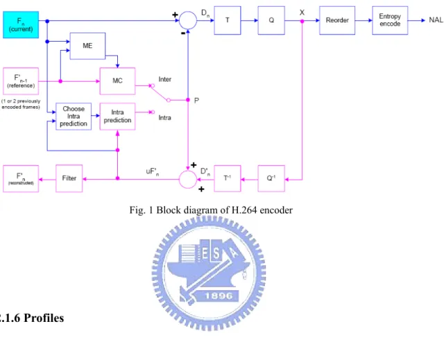
A simplified encoding flow of H.264 is shown in Fig. 1[7]. A video frame is first partitioned into a number of 16x16 macroblocks. Then, each macroblock goes through the intra-prediction or the inter-prediction unit called motion estimation(ME). The intra prediction unit uses the neighboring block data to predict the current block. The inter-prediction uses reference frames to predict the current frame. Each predictor has a number of modes. A good design should pick up the best mode with the lowest rate and distortion. The prediction residuals are then transformed, quantized and further entropy-coded into the output bitstream. In order to continue operating on the
6
next incoming frame, the quantized current frame is reconstructed and stored. The decoder data flow is the reverse of the encoder flow.
Fig. 1 Block diagram of H.264 encoder
2.1.6 Profiles
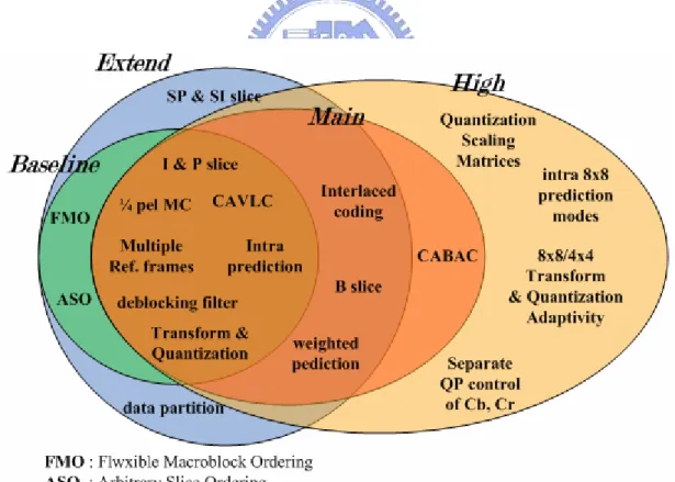
A profile defines a set of coding tools or algorithms that can be used in generating a conforming bit stream. In the initial H.264/AVC standard, three basic profiles were established to address these application domains: the Baseline, Main, and Extended profiles. The Baseline profile was designed to minimize complexity and provide high robustness and flexibility for use over a broad range of network environments and conditions; the Main profile was designed with an emphasis on compression coding efficiency capability; and the Extended profile was designed to combine the robustness of the Baseline profile with a higher degree of coding efficiency and greater network robustness and to add enhanced modes useful for such applications as flexible video streaming.
7
While having a broad range of applications, the initial H.264/AVC standard (as it was completed in May of 2003), was primarily focused on "entertainment-quality" video, based on 8-bits/sample, and 4:2:0 chroma sampling. Given its time constraints, it did not include support for use in the most demanding professional environments, and the design had not been focused on the highest video resolutions. To address the needs of these most-demanding applications, a continuation of the joint project was launched to add new extensions to the capabilities of the original standard. These extensions, originally known as the "professional" extensions, were eventually renamed as the "fidelity range extensions" (FRExt)[8] to better indicate the spirit of the extensions. These included:
Supporting an adaptive block-size for the residual spatial frequency transform
Supporting encoder-specified perceptual-based quantization scaling matrices Supporting efficient lossless representation of specific regions in video
content.
The FRExt project produced a suite of four new profiles collectively called the High profiles:
The High profile (HP), supporting 8-bit video with 4:2:0 sampling, addressing high-end consumer use and other applications using high-resolution video without a need for extended chroma formats or extended sample accuracy
The High 10 profile (Hi10P), supporting 4:2:0 video with up to 10 bits of representation accuracy per sample.
8
up to 10 bits per sample, and ♦ The High 4:4:4 profile (H444P), supporting up to 4:4:4 chroma sampling, up to 12 bits per sample, and additionally supporting efficient lossless region coding and an integer residual color transform for codingRGB video while avoiding color-space transformation error.
All of these profiles support all features of the prior Main profile, and additionally support an adaptive transform blocksize and perceptual quantization scaling matrices. The High profile adds more coding efficiency to what was previously defined in the Main profile, without adding a significant amount of implementation complexity. Fig. 2 shows the relationship of Baseline, Main, Extended and High profiles.
9
2.2 INTRA PREDICTION
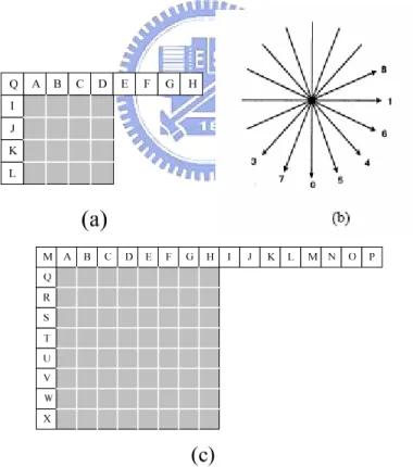
In contrast to previous video coding standards like H.263 and MPEG-4, where intra prediction is performed in the transform domain, in H.264/AVC it is always conducted in the spatial domain. By referring to neighboring samples of coded blocks which are to the left or/and above current predicted block, most of the energy in the block can be removed in the intra prediction process. With the help of intra prediction, the compression performance of small block-size transform is enhanced. For luma components, there are nine 4x4 prediction modes and four 16x16 prediction modes. Furthermore, additional nine 8x8 prediction modes are added in high profile.
Fig. 3 (a) Intra_4_4 prediction is conducted for samples a-p of a block using samples A-Q. (b) Eight “prediction directions” for 4x4 or 8x8 intra prediction.
10
When using the 4x4 or 8x8 intra prediction, each 4x4 or 8x8 block is predicted from spatially neighboring samples as shown inFig. 3(a)(c). For each block, one of nine direction modes can be chosen. In addition to “DC” prediction (where one value is used to predict the entire 4x4/8x8 block), eight directional prediction modes are specified as illustrated in Fig. 3(b).
For 16x16 prediction modes, the whole luma component of a macroblock is predicted. Four prediction modes are supported. They are vertical prediction, horizontal prediction, DC prediction and plane prediction. The chroma components are predicted using a similar prediction technique as that in the 16x16 prediction since chroma components are usually smooth over large areas. Intra prediction and all other forms of prediction are not used while across slice boundaries to keep all slices independent of each other.
2.3 INTER FRAME PREDICTION
The inter prediction in H.264/AVC is a block matching based motion estimation and compensation technique. It can remove the redundant inter-frame information efficiently. Each inter macroblock corresponds to a specific partition into blocks used for motion compensation. For the luma components, partition with 16x16, 8x16, 16x8 and 8x8 are supported by the syntax. Once the 8x8 partition is chosen, additional syntax is transmitted to specify whether the 8x8 partition is further partitioned into 8x4, 4x8 or 4x4 blocks. Fig. 4 illustrates these partitions.
11
Fig. 4 Inter macroblock partitions
The prediction information for each MxN block is obtained by displacing an area of the corresponding reference frame, which is determined by the motion vector and reference index. H.264/AVC supports quarter pixels accurate motion compensation. The sub-pel prediction samples are obtained by interpolation of integer position samples. For the half-pel position, the prediction value is interpolated by a one-dimensional 6-tap FIR filter horizontally and vertically. For the quarter-pel position, the interpolation value is generated by averaging the samples at integer-pel and half-pel position. Fig. 5 shows the fractional sample interpolation.
12
The prediction values for the chroma component are always obtained by bilinear interpolation. Since the chroma components are down-sampled, the motion compensation for chroma has one-eighth position accuracy since that for luma has one-fourth position accuracy.
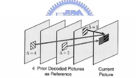
The motion vector components are differentially coded using either median or directional prediction from neighboring blocks. Besides, H.264/AVC supports multiple reference frame prediction. That is, more than one prior coded frame can be used as reference for motion compensation as Fig. 6 illustrated.
Fig. 6 Multiple reference frame motion compensation
2.4 TRANSFORM
Similar to previous video coding standards, H.264/AVC utilizes transform coding of the prediction residual. However, instead of fractional discrete cosine transform applied by previous standard, an integer transform with similar properties
13
as DCT is adopted. Thus, the inverse-transform mismatches can be avoided due to the exact integer operation of transform. The transformation is applied to 4x4 blocks. But for 16x16 intra luma prediction or 16x16, 16x8, and 8x16 inter prediction, 8x8 DCT is applied in high profile of H.264. Furthermore, for the 16x16 intra luma prediction or chroma prediction, extra Hadamard transform is applied on the DC coefficients of 4x4 blocks.
2.5 QUANTIZATION
A quantization parameter is used for determining the quantization of transform coefficients in H.264/AVC. The parameter can take 52 values. The quantized transform coefficients of a block generally are scanned in a zig-zag order and transmitted using entropy coding methods. The 2x2 DC coefficients of the chroma component are scanned in the raster-scan order. The transform is simplified to integer operation because some operation is performed in the quantization stage. The quantization parameter is different between 4x4 and 8x8 DCT in high profile of H.264.
2.6 ENTROPY CODING
In H.264/AVC, there are two methods of entropy coding. The simpler entropy coding method, UVLC, uses exp-Golomb codeword tables for all syntax elements except the quantized transform coefficients.For transmitting the quantized transform coefficients, a more efficient method called Context-Adaptive Variable Length
14
Coding (CAVLC) is employed. In this scheme, VLC tables for various syntax elements are switched depending on already transmitted syntax elements.
In the CAVLC entropy coding method, the number of nonzero quantized coefficients (N) and the actual size and position of the coefficients are coded separately. After zig-zag scanning of transformed coefficients, their statistical distribution typically shows large values for the low frequency part and becomes to small values later in the scan for the high-frequency part.
The efficiency of entropy coding can be improved further if the Context-Adaptive Binary Arithmetic Coding (CABAC) is applied. In H.264/AVC, the arithmetic coding core engine and its associated probability estimation are specified as multiplication-free low-complexity methods using only shifts and table look-ups. Compared to CAVLC, CABAC typically provides a reduction in bit rate between 5%–15%.
15
Chapter 3 Review of FME Search Algorithms
3.1 SEARCH ALGORITHM IN THE REFERENCE SOFTWARE [12] 3.1.1 Algorithm
: Integer pixel
: half pixel
: quarter pixel
Fig. 7 Search algorithm in the reference software
Fig. 7 details the search algorithm for the Fractional-pel ME(FME) process according to the reference software[12]. The search process in fractional motion estimation is typically divided into two parts. The first part consists of half-pel motion estimation, where specific pixels at half-pel spacing are searched for comparison. The second part consists of quarter-pel motion estimation, where pixels at quarter-pel spacing centered around a search point obtained in the first part are used for comparison.
16
In the first part of half-pel ME, a cost value for each of eight search points in a square search pattern surrounding the integer spaced pel called search center is calculated. A cost value calculation for the search center is also performed. The search point with the lowest cost value is then selected as the quarter-pel motion estimation search center in the next step. The fractional motion estimation step utilizes an additional eight fractional search points displaced around the search center at quarter-pel spacing. A total of 17 search points (1 search point from integer pel, 8 search points from half-pel ME and 8 search points from quarter-pel motion estimation) are searched and compared in a single round of the traditional ME procedure according to the reference software.
3.1.2 Hardware implementation[16]
In the hardware implementation of the above algorithm in [16], firstly, reference pixels are loaded to interpolation unit and then demanded sub-pixels are generated. After that, the demanded sub-pixels and current MB pixels go into the 4x4 block PU which is responsible for residual generation and Hadamard transform. It processes 4x4 element blocks decomposed from sub-block in sequential order. There are nine 4x4 block PU’s processing nine candidates around the refinement center simultaneously. Finally, nine accumulators accumulating the SATD of each 4x4 element block and corresponding MV cost and sent it to the compare unit for determining the best candidate.
17
3.2 FIVE CANDIDATES ALGORITHM [15] 3.2.1 Algorithm
Fig. 8 Five candidates search algorithm
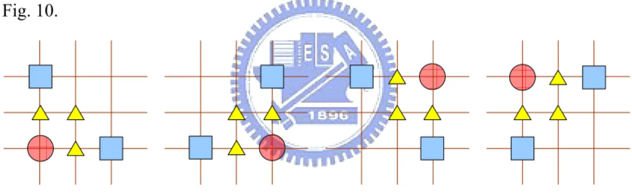
The author of [15] finds that the error surface of sub-pel motion estimation is unimodal in most cases. Therefore, he biases his second search step near the center and just examines the neighborhood position around the points with low cost value. Fixed half-pel search pattern and adapt quarter-pel search patterns are applied in his search algorithm.
Step1: Calculate the five search points of the center and the four half-pel points. Step2: Adaptively select the search pattern depending on the best three search positions of the first step. If the integer-pel has minimum cost, the algorithm will bias the search pattern to the search center, as shown in Fig. 8(a). Otherwise, it will bias the search pattern away from the search center, as shown in Fig. 8(b). The detail of each case is shown below.
18
Case 1: When the center has minimum cost, the second and third best search positions aren’t near each other. It will choose the three search points between the best and the second best ones, as shown in Fig. 9.
Fig. 9 Refine position in case 1
Case 2: The minimum cost point falls on search center and the second best positions is neighbor to the third one. It will choose the “L” shape pattern as shown in Fig. 10.
Fig. 10 Refine position in case 2
Case 3: The best two search positions are at the four half-pel positions and neighboring to each other. It will choose the three points in the “L” shape between the best two as shown in Fig. 11.
19
Case 4: When the best two search points are at the four half-pel positions and not neighboring to each other. It will search the four candidates around the best search point as shown in Fig. 12.
Fig. 12 Refine position in case 4
3.2.2 Hardware implementation
Search window data rearrangement
Adaptive Search Pattern Selection Unit
4x4 Block
PU
Compare and determine quarter search pattern type
Interpolation Unit
Control
Mode
MV
Ref frame
data
Original MB
data
Best MV Early Termination Unit Residual buffer 4x4 Block PU 4x4 Block PU 4x4 Block PU 4x4 Block PUMB header
20
Fig. 13 shows the block diagram of the architecture in [15]. The core procedure of FME includes interpolation, residual generation and Hadamard transform. The interpolation unit interpolates the fractional pixels by 6-tap filter. Due to the irregular search pattern used in second step, interpolated fractional pixels should be adaptively selected before been send into PU.
The 4x4 block PU has four times parallelization of horizontal adjacent pixels and is in charge of residual generation and Hadamard transform. It processes 4x4 element blocks decomposed from sub block in sequential order.
SATD generated form PUs and MB header included motion vector, reference frames and type of block sizes are send into the compare and determination unit for the Largrangian mode decision. Mode decision is combined with comparator. In the first search step, we should know not only the best position but also second and third places. Then, the information of the first step is send into selection unit to choose the input of the next step.
21
3.3 QUADRATIC PREDICTION BASED FME [14]
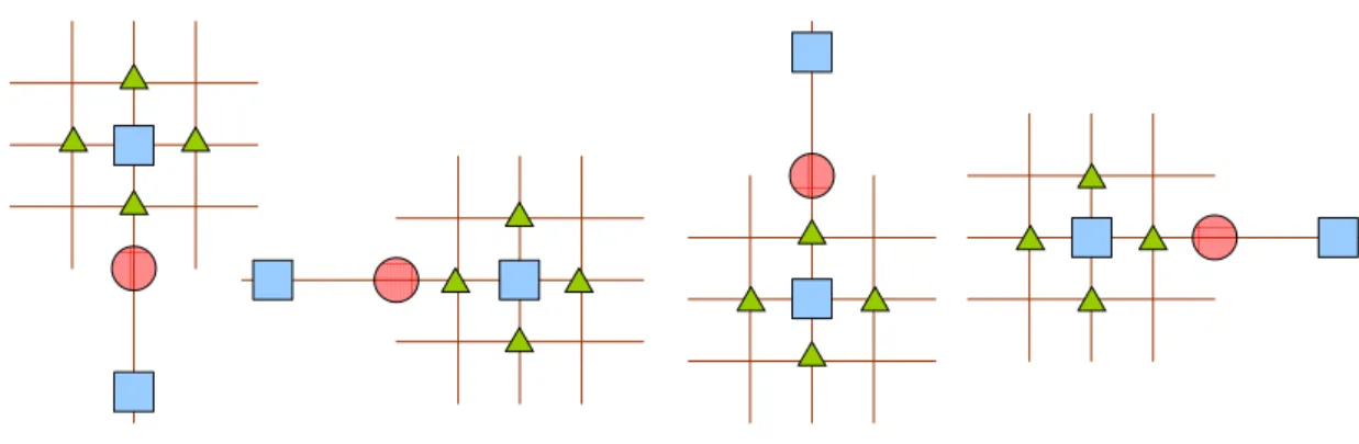
H1 C H2
V1
V2
: Integer pixel
(xp, yp)
: diamond search point : (xp, yp)
Fig. 14 The integer-pixel search positions within the "local" fractional-pel ME search area.
The fast algorithm in [14] uses a mathematical model to predict the best position at quarter-pel position. In this paper, a “degenerate” quadratic prediction function is used to model the matching error function within the fractional-pel ME search area, which is given by E Dy Cy Bx Ax y x F( , )= 2 + + 2 + +
where x and y are local x and y coordinates of a search position at fractional-pel accuracy and A, B, C, D, and E are parameters to be determined. As shown in Fig. 14, a fractional-pel ME search area with search range=1 pixel contains 9 integer-pel search positions. The five matching error values of the five integer-pel search positions, C, H1, H2, V1, and V2 are known in the previous integer-pel ME search procedure. These five SADs are employed to determine the five parameters, A, B, C, D, and E in the equation.
In Fig. 1, the local coordinates of the five integer pixel positions C, H1, H2, V1, and V2 are (0,0), (-1,0), (1,0), (0,-1), and (0,1). Then we have
22 ⎪ ⎪ ⎪ ⎩ ⎪⎪ ⎪ ⎨ ⎧ + + = + − = + + = + − = = E B A H F E B A H F E D C V F E D C V F E C F ) 2 ( ) 1 ( ) 2 ( ) 1 ( ) (
For simplicity, let ⎪ ⎪ ⎩ ⎪ ⎪ ⎨ ⎧ − = − = − = − = C V F L C V F K C H F J C H F I ) 1 ( ) 2 ( ) 1 ( ) 2 ( Then we have
(
)
(
)
(
)
⎪ ⎪ ⎪ ⎩ ⎪⎪ ⎪ ⎨ ⎧ = − = + = − = + = ) ( 2 / 2 / 2 / 2 / C F E L K D L K C J I B J I AIt is assumed that F(x, y) is continuous (smooth) within the “local” fractional-pel search area, to obtain the minimum F(x, y), and then the differential operation can be performed on F(x, y) with respective to x and y, respectively and then set it to zero. The solution to the above differential equations is,
⎪⎩ ⎪ ⎨ ⎧ = = ≠ − = 0 , 0 0 , 2 A x A A B x p p , ⎪⎩ ⎪ ⎨ ⎧ = = ≠ − = 0 , 0 0 , 2 C y C C D y p p
where
(
x
p,
y
p)
is the best position in quarter-pel accuracy.After determine the best position, the author does the first diamond search around it. Then, it refines around the best point until it is center-located. This algorithm needs at least two iterative loops and additional memory to store information from integer-pel motion estimation. Therefore, it is not suitable for hardware implementation.
23
3.4 CENTER-BIASED FRACTIONAL-PEL SEARCH (CBFPS)[13]
(a)
(b)
Fig. 15 (a) Sub-pel motion vector distribution using the Full Search algorithm versus the (0,0) MV (b) Sub-pel motion vector distribution using the Full Search algorithm versus the median predictor.
The concept behind the center-biased FME[13] is that the probability of finding the motion vector around frac_pred_mv is higher than that around (0,0). Fig. 15(a) shows the sub-pel motion vector distribution using the Full Search Algorithm versus the (0,0) MV and Fig. 15(b) shows that versus the median predictor. The distribution versus the median predictor is more center distributed than versus (0,0). Hence it can be concluded that we have higher probability to find the accurate sub-pel MV around the median predictor than around the (0,0) MV.
The center-biased FME[13] uses the information of predicted motion vector (pred_mv). It first calculates the fractional predicted motion vector(frac_pred_mv) :
β
)% _ ( _ _ pred mv pred mv mv frac = − (1)where pred_mv here is defined as the fractional pixel unit. mv is the integer pixel motion vector after IME process, and mv is also in fractional pel unit. % is the mode operation, β=4 in 1/4-pel case and β=8 in 1/8-pel case. frac_pred_mv is the predicted
24
fractional motion vector and indicates only fractional position. Then, it compares the cost at (0, 0) and frac_pred_mv and does the first diamond search around the lower cost one. After that, it refines around the best point until it is center-located. However, this algorithm still needs at least two iterative loops and thus is not suitable for low latency hardware design.
25
3.5 FAST FRACTIONAL-PEL ME USING MATHEMATICAL MODEL[17][23] 3.5.1 Algorithm
Fig. 16 The integer and half pixels within the fractional-pel ME search area.
The author in [17] implements the method of [23] and extends it to quarter-pel precision. He uses a mathematical model to estimate SADs at quarter-pel position. The mathematical model used to approximate the surface defined by the nine integer pixels is as following: 9 8 2 7 6 5 2 4 2 3 2 2 2 2 1 ) , (x y C x y C x y C x C xy C xy C x C y C y C f = + + + + + + + + …..(1)
26
⎥
⎥
⎥
⎥
⎥
⎥
⎥
⎥
⎥
⎥
⎥
⎥
⎦
⎤
⎢
⎢
⎢
⎢
⎢
⎢
⎢
⎢
⎢
⎢
⎢
⎢
⎣
⎡
⋅
⎥
⎥
⎥
⎥
⎥
⎥
⎥
⎥
⎥
⎥
⎥
⎥
⎦
⎤
⎢
⎢
⎢
⎢
⎢
⎢
⎢
⎢
⎢
⎢
⎢
⎢
⎣
⎡
−
−
−
−
−
−
−
−
−
−
−
=
⎥
⎥
⎥
⎥
⎥
⎥
⎥
⎥
⎥
⎥
⎥
⎥
⎦
⎤
⎢
⎢
⎢
⎢
⎢
⎢
⎢
⎢
⎢
⎢
⎢
⎢
⎣
⎡
9 8 7 6 5 4 3 2 1 9 8 7 6 5 4 3 2 11
1
1
1
1
1
1
1
1
1
1
1
0
0
0
0
0
0
1
1
1
1
1
1
1
1
1
1
0
0
1
1
1
1
0
0
1
0
0
0
1
0
0
0
0
1
0
0
1
0
1
1
0
0
1
1
1
1
1
1
1
1
1
1
1
1
0
0
0
0
0
0
1
1
1
1
1
1
1
1
1
C
C
C
C
C
C
C
C
C
f
f
f
f
f
f
f
f
f
……….(2)Its 9 coefficients can be determined by 9 integer-pixel precision SADs around (0, 0), as shown in Fig. 16. We can obtain 9 coefficients by the inverse matrix of Eq. (2), as shown in Eq. (3).
⎥
⎥
⎥
⎥
⎥
⎥
⎥
⎥
⎥
⎥
⎥
⎥
⎦
⎤
⎢
⎢
⎢
⎢
⎢
⎢
⎢
⎢
⎢
⎢
⎢
⎢
⎣
⎡
⋅
⎥
⎥
⎥
⎥
⎥
⎥
⎥
⎥
⎥
⎥
⎥
⎥
⎦
⎤
⎢
⎢
⎢
⎢
⎢
⎢
⎢
⎢
⎢
⎢
⎢
⎢
⎣
⎡
−
−
−
−
−
−
−
−
−
−
−
=
⎥
⎥
⎥
⎥
⎥
⎥
⎥
⎥
⎥
⎥
⎥
⎥
⎦
⎤
⎢
⎢
⎢
⎢
⎢
⎢
⎢
⎢
⎢
⎢
⎢
⎢
⎣
⎡
9 8 7 6 5 4 3 2 1 9 8 7 6 5 4 3 2 11
1
1
1
1
1
1
1
1
1
1
1
0
0
0
0
0
0
1
1
1
1
1
1
1
1
1
1
0
0
1
1
1
1
0
0
1
0
0
0
1
0
0
0
0
1
0
0
1
0
1
1
0
0
1
1
1
1
1
1
1
1
1
1
1
1
0
0
0
0
0
0
1
1
1
1
1
1
1
1
1
f
f
f
f
f
f
f
f
f
C
C
C
C
C
C
C
C
C
……….(3)It substitute these 9 coefficients into the original mathematical model (Eq.(2)). In the next step, SADs at the neighboring half-pixel positions (h1, h2, …, h9) can be obtained by replacing x and y in Eq.(2) with its coordinates. The position which causes minimum SAD is the half-pixel precision MV.
After finding the minimum SAD at half-pixel level, the author resets the origin (0, 0) to the position pointed to by half-pel MV and find the minimum SAD at quarter-pel precision similarly.
27
3.5.2 Hardware implementation
Fig. 17 Top-level architecture in [17]
Fig. 17 depicts the top-level architecture in [17]. It consists of two parts: FME and mode decision. For each variable-size block, the FME receives from IME an integer MV and nine associated SADs (one for the best integer position and eight around the best) and outputs a fractional MV and a minimum SAD at quarter-pixel precision. The mode decision engine receives SAD and fractional MV from FME and reference index from IME. It produces the chosen modes and associated MVs of macroblock and submacroblocks. The architecture of FME is a direct implementation of Eq (3)). In the first step, FME receives nine SADs from IME and figures out 9 related SADs at half-pixel precision. Then, the comparator finds the minimum half-pixel SAD and MV Refiner adjusts integer MV to half-pixel precision according to the comparison result.
28
3.6 SUMMARY
Although the search algorithm illustrated in the reference software does manage to sufficiently locate suitable search points for the motion vector refinement process, the excess amount of search points may result in significant delays in the encoding process. This search algorithm for the FME process may possess too many search points to visit within one motion vector refinement process. Furthermore, although this algorithm is suitable for hardware[16], the Fractional-Pel ME process requires two iterative search loops of interpolation and Hadamard transform to calculate the SATD cost. Therefore, the process takes too much cycle time in hardware implementation.
The center based fractional pixel search (CBFPS)[13] and the quadratic prediction based fractional ME algorithm[14] are software-oriented and exhibit irregular data flow and thus are not suitable for hardware design. Although the algorithm in [17] is suitable for hardware, it has more than 0.2dB degradation in PSNR and needs additional hardware to generate residual. The five candidates algorithm[15] which is our previous work is also suitable for hardware and can reduce the processing unit from nine to five to save hardware cost. However, from the hardware viewpoint it still suffers from long computation cycles as others. That is because it still takes two iterative search loops, one on half-pels and one on quarter-pels[16]. Thus, it only reduces the processing element but do not reduce the cycle count in the hardware implementation. This problem will pose a strict limit on the HDTV sized applications since FME will take a lot of cycles and dominate the whole pipelining cycle time.
29
Besides, all of these algorithms and designs do not consider the costly 8x8 SATD (sum of absolute transformed difference) computations in the high profile of H.264. In H.264 high profile standard, blocktypes larger than 8x8, i.e. 16x16, 16x8, and 8x16, pass through 8x8 DCT rather than 4x4 DCT before entropy coding. Hence, in FME stage, the SATD of blocktypes larger than 8x8 is calculated by 8x8 Hadamard transform rather than Hadamard 4x4 transform. However, 8x8 Hadamard transform causes the interpolation unit and transform units to increase their area. Thus, the FME hardware for high profile standard should be much larger than that for baseline or main profile standard.
To solve above problems, we presents a single iteration fast FME algorithm and its architecture suitable for HDTV and high profile applications. The proposed algorithm can complete the quarter-pel precision motion search by only examining six search points in one search step instead of 17 search points in two search steps in the reference software[12]. Thus, we can reduce the number of SATD units since we only search 6 candidates. Besides, the cycle count is also halved by using only one search step. Furthermore, to avoid the costly 8x8 SATD computations with 8x8 Hadamard transform, we use the 4x4 Hadamard transform units. Thus, we can achieve smaller area and fewer cycle counts at the same time.
30
Chapter 4 A Single Iteration Fractional-pel
Motion Estimation Algorithm
4.1 PROPOSED SINGLE ITERATION ALGORITHM 4.1.1 Proposed SIFME Algorithm
frac_pred_mv
(0,0)
Fig. 18 The proposed SIFME algorithm flow on two square points, (0,0) and frac_pred_mv, and four triangle point around frac_pred_mv in one quarter-pel distance
Inspired by the center-biased FME, we modify it by searching six candidates in only one loop and no refined search as shown in Fig. 18. The six candidates includes (0,0), frac_pred_mv and four diamond points around frac_pred_mv. (0, 0) is included for low texture and low motion sequences. More search points are placed around
frac_pred_mv since the best fractional motion vector is more often around frac_pred_mv than around (0, 0).
31
search pattern. The quarter-pel search pattern is selected according to the ranking of cost values for each specific search point, and provides search points in a certain area to approach the global minimum cost in the search window. In an effort to reduce confusion, the search points deduced in the quarter-pel ME stage will be referred to as quarter-pel search points. However, both types of search points serve the same purpose in providing matching points for the ME process.
Once the quarter-pel search pattern is determined (further below), cost values for the quarter-pel search points of the fractional search pattern are then calculated. The cost values attained here are used in conjunction with the cost data accumulated from search points in the first stage to determine whether the current macroblock is a suitable match to the reference macroblock. The entire search pattern therefore comprises the half-pel search pattern used in the first stage and the quarter-pel search pattern used the second stage for fractional ME.
32
4.1.2 Analysis of prediction accuracy and search point
The method of the present invention manages to arrive at a comparable matching accuracy while reducing the total search points and processing time. Table 1 shows the prediction correctness compared with the algorithm in the reference software under different quantization parameter (QP). The prediction accuracy is defined as if the search fractional MV by the fast algorithm is the same as that in the reference software in both x and y axis. This result shows that it can still have about 60~90 % of prediction accuracy though the proposed algorithm had ignored more than 88% search points.
Table 1 Hit rate of motion vector (mvx and mvy) compared to the algorithm adopted by JM
CIF size, 300 frame, IPPP, ProfileIDC=100, RDO off QP container foreman mobile stefan
10 82.31% 61.80% 74.10% 62.20% 16 85.11% 68.60% 76.30% 70.70% 22 82.18% 70.97% 76.70% 75.70% 28 90.21% 78.90% 79.00% 79.40% 34 94.41% 86.40% 82.30% 82.83% 40 94.71% 91.10% 86.10% 85.40%
In addition, our algorithm is more accurate in higher QP condition. The reason may be that our algorithm tends to find the motion vector which is similar to the motion vector predictor(mvp) and thus has lower motion vector cost. Therefore, in high QP condition where motion vector cost dominates rather than SATD cost does, motion vectors found by our algorithm have lower motion vector cost and become more accurate.
33
Table 2 provides the search point comparisons with other algorithms. The proposed algorithm needs the fewest search points compared with other search algorithms, 64% reduction compared to reference software and 33% reduction compared to the algorithm in [15]. This significantly reduces the hardware processing time required by a related compression encoder or a microprocessor for use in video compression. Besides, our algorithm does not need the second step search and saves the additional interpolation time in the second step. Table 3 shows the comparisons for hardware implementation. The proposed algorithm searches only six candidates and needs only six PUs. Besides, since in hardware implementation, all candidates in the same step are processing in parallel, cycle time is dependent on the number of iterative steps, not number of candidates. With one loop design, our design just takes about only half of cycles compared to that with reference software[16] and fast algorithm in [15].
Table 2 Search point comparisons for different algorithms
Search points
JM 9.8[12] 17
Quadratic Prediction[14] 6 + multiple diamond search (Total <=11) CBFPS[13] 6 + multiple diamond search
Y. J. Wang[15] 8~9
Proposed 6
Table 3 Comparisons of number of processing unit(PU) and number of iterative search steps
# of PU # of iterative search step
T. C. Chen[16] 5 2
Y. J. Wang[15] 9 2
34
4.1.3 Proposed SATD cost of 4x4 Hadamard transform algorithm
In high profile standard of H.264, residual of block size larger than 8x8 are passed through 8x8 DCT rather than 4x4 one. Thus, in the reference software, it adopts 8x8 Hadamard transform for SATD calculation for block size larger than 8x8[18]. Though Hadamard transform is greatly simplified, one 8x8 Hadamard transform unit still consumes about four times area than that of 4x4 one. For six PUs in our design, six 8x8 transform will be required and thus cost a lot of area cost. Moreover, the area of interpolation unit will also increase. To solve this area problem, we propose to use 4x4 Hadamard for all SATD calculation disregarding of the block size.
Table 4 shows the simulation results of our algorithm with different SATD strategy. We set only the first frame to be I-frame because inserting I-frame periodically will ease up the effect of our algorithm. All the data are in Table 4 compared with the reference software. As shown in the table, the results with 4x4 and 8x8 Hadamard transform are similar except for low motion sequences like container at high QP situations. That is quite acceptable since the bit rate at that condition is quite low and any increase will be large in terms of that bit rate. As the 4x4 transform unit only consumes 25% area cost of 8x8 one, we choose to calculate SATD by 4x4 Hadamard transform that has similar performance and saves about 75% of area cost in PU and 60% of area cost in the total FME module.
35
Table 4 Simulation results of SIFME with different SATD methods when compared to the reference software[12]
CIF size, 300 frame, only first frame is I-frame, ProfileIDC=100, RDO off, Search range = 32
SIFME with 4x4 Hadamard transform
container foreman mobile&calendar stefan QP ΔPSNR (dB) Δbit rate ΔPSNR (dB) Δbit rate ΔPSNR (dB) Δbit rate ΔPSNR (dB) Δbit rate 10 -0.03 -0.75% -0.05 0.04% -0.04 -0.24% -0.04 0% 16 0 -0.28% -0.07 1.03% -0.06 0.16% -0.05 0.30% 22 -0.03 -0.37% -0.09 0.89% -0.08 0.06% -0.06 0.50% 28 0.03 0.46% -0.09 1.50% -0.07 0.47% -0.07 1.24% 34 0.04 2.11% -0.12 1.35% -0.07 1.73% -0.10 1.57% 40 -0.03 4.36% -0.08 -0.36% -0.08 2.30% -0.13 1.02% SIFME with 8x8 Hadamard transform
container foreman mobile&calendar stefan QP ΔPSNR (dB) Δbit rate ΔPSNR (dB) Δbit rate ΔPSNR (dB) Δbit rate ΔPSNR (dB) Δbit rate 10 -0.02 -0.19% -0.02 -0.19% -0.03 0.34% -0.03 0.31% 16 -0.03 -0.35% -0.03 -0.35% -0.03 0.64% -0.04 0.68% 22 -0.01 -0.25% -0.01 -0.25% -0.06 0.79% -0.06 1.06% 28 0.03 0.19% 0.03 0.19% -0.06 1.16% -0.07 1.86% 34 -0.02 0.72% -0.02 0.72% -0.06 1.59% -0.08 1.97% 40 0.02 2.53% 0.02 2.53% -0.09 -0.10% -0.11 -0.04%
36
4.2 SIMULATION RESULT & COMPARISON
Table 5 shows the simulation results of the proposed SIFME with 4x4 Hadamard transform algorithm compared with that of reference software for 720p and 1080p sequences. Since our hardware architecture is used for high profile and HDTV size video, we care more about the performance on 1080p and 720p size sequences rather than that on CIF size sequences. Comparing the results of Table 4, Table 5, and Table 6, we can find that our algorithm has better performance on large size sequences than CIF size sequences, which matches our goal. We can also find that our algorithm greatly reduces computation time of FME. The proposed algorithm can speedup the FME part by up to 4 times compared to the reference software. The reason is due to the reduction of search candidates, and use 4x4 Hadamard transform instead of 8x8 one.
For the result on 720p size sequence shown in Table 5, the PSNR degradation is around 0~0.08dB and the bit rate even decreases on many sequences. For low motion sequence like container in Table 4 and mobcal in Table 5 at high QP situation, the bit rate may increase. That is quite acceptable since the bit rate at that condition is quite low and any increase will be large in terms of that bit rate. However, for most 720p sequences, the bit rate even decreases. The reason may be that our algorithm tends to find the motion vector which is similar to the motion vector predictor(mvp) and thus saves bits for coding motion vectors.
37
Table 5 PSNR & bit rate comparison for different 720p sequences and QPs. Speed up is only the performance in fractional ME part
JM9.8, 720p, 300 frames, only first frame is I-frame, ProfileIDC=100, RDO off, search range=64
SIFME with 4x4 Hadamard transform
mobcal parkrun shields stockholm
QP ΔPSN R(dB) Δbit rate speed up ΔPSN R(dB) Δbit rate speed up ΔPSN R(dB) Δbit rate speed up ΔPSN R(dB) Δbit rate speed up 10 -0.04 -0.77% 4.0 -0.02 -0.77% 3.9 -0.04 -0.42% 3.6 -0.04 0.05% 3.8 16 -0.04 -1.07% 3.6 -0.04 -0.99% 3.7 -0.08 -1.27% 3.7 -0.08 -0.86% 3.6 22 -0.01 -1.08% 4.0 -0.05 -1.42% 3.9 -0.04 -1.54% 3.9 -0.05 -1.50% 3.7 28 -0.01 -0.36v 3.9 -0.04 -0.63% 3.9 -0.02 -0.36% 3.6 -0.02 -0.71% 3.8 34 -0.05 3.20% 3.9 -0.05 -0.14% 3.8 -0.03 0.30% 3.6 -0.01 -1.87% 3.7 40 -0.06 4.28% 3.7 -0.04 -0.70% 4.1 -0.01 -7.05% 3.5 0 -8.86% 3.7
Table 6 PSNR & bit rate comparison for different 1080p sequences and QP
JM9.8, 1080p, 200 frames, only first frame is I-frame, ProfileIDC=100, RDO off, SearchRange=128 SIFME with 4x4 Hadamard transform
blue sky pedestrian riverbed rush hour sation2 sunflower tractor
QP ΔPSN R(dB) Δbit rate ΔPSN R(dB) Δbit rate ΔPSN R(dB) Δbit rate ΔPSN R(dB) Δbit rate ΔPSN R(dB) Δbit rate ΔPSN R(dB) Δbit rate ΔPSN R(dB) Δbit rate 10 -0.06 -1.14% -0.07 -1.41% -0.07 -0.53% -0.07 -1.13% -0.06 -0.64% -0.11 -0.27% -0.08 0.38% 16 -0.05 -0.74% -0.05 -0.68% -0.09 -1.85% -0.06 0.62% -0.07 -1.08% -0.10 -0.11% -0.12 -0.16% 22 -0.03 -1.20% -0.05 -1.32% -0.07 -2.11% -0.04 0.02% -0.08 -1.65% -0.07 -2.53% -0.11 -1.38% 28 0 0.08% -0.02 -1.03% -0.08 -1.14% 0.02 0.72% -0.01 4.70% -0.01 -1.71% -0.09 -0.66% 34 0.01 2.40% 0.07 0.55% -0.03 0.48% 0.13 1.68% 0.03 -2.43% -0.02 -3.54% -0.03 1.10% 40 0.08 4.47% 0.16 0.68% 0.06 1.45% 0.22 1.44% 0.13 -7.55% 0.02 -5.07% 0 2.36%
38
Table 6 shows the result on 1080p sequence. The result at low QP situation is quite the same as that on 720p sequence. However, at high QP condition, the PSNR performance of our algorithm is even better than that of the reference software. The reason may be that the accurate motion vector is getting closer to motion vector predictor at high QP condition, and hence the accurate fractional one is getting closer to frac_mv_pred illustrated in Sec. 4.1 .
Summing the information in Table 4, Table 5, and Table 6, we can conclude that our proposed algorithm ignore 88% search point and achieve nearly 4 times speed up with only less than 0.13 dB PSNR degradation and 4.47% bit rate increase. For some 720p or 1080p sequences, our algorithm even has better PSNR quality or less bit rate than that of JM software[12]. The rate distortion curves are shown in Fig. 19, Fig. 20, and Fig. 21. In each figure, the curve of our proposed algorithm is very close to that of the method used in JM software[12].
25 30 35 40 45 50 0 1000 2000 3000 4000 5000 6000 7000 8000 kbits/sec PS N R (d B ) JM 9.8 our proposed
39 25 30 35 40 45 50 0 20000 40000 60000 80000 100000 kbits/sec PSN R( dB) JM 9.8 our proposed
Fig. 20 Rate distortion curve of the four 720p size sequences
30 35 40 45 50 0 30000 60000 90000 120000 150000 kbits/sec PSN R (d B ) JM 9.8 our proposed
40
Table 7 shows the simulation results of the proposed algorithm and reference previous works compared with that of the reference software. We integrate our algorithm into the reference software and use the full search algorithm for integer ME for fair comparison. It can be found that our algorithm greatly reduces computational complexity but only leads to a small amount of quality loss. Our algorithm speeds up more compared with our previous work[15] with the same PSNR quality and less bit rate increase. The algorithm in [13] has better performance in PSNR and bit rate than our algorithm does because we cut the number of iteration to one and simplify the cost function of SATD. Nevertheless, this algorithm has many number of iteration and hence is not suitable for hardware implementation.
Table 7 Simulation result when QP = 28, speed up is only the performance in fractional ME part. RDO is off, reference frame number = 1, 300f, CIF
QP = 28 Stefan Mobile Foreman Coastguard News # of iteration bit rate 1441.14 1888.69 498.62 1127.87 223.72 PSNR 35.36 33.75 36.24 34.52 38.12 JM 9.8 [12] time (sec) 491.604 471.993 496.974 488.039 450.37
1
△bit rate(%) 2.2843 2.36407 1.780915 1.070159 2.23494 △PSNR(dB) -0.09 -0.11 -0.07 -0.04 -0.06 Y. J. Wang [15] speed up 2.34227 2.24167 2.361651 2.283373 2.247872
△bit rate(%) -0.1524 -0.0822 -0.7819 -0.402 0.2294 △PSNR(dB) -0.01 -0.01 -0.03 -0.01 0 CBFPS [13] speed up 2.163 2.265 2.249 2.307 2.638> 2
△bit rate(%) 1.2408 0.4657 1.5022 -0.9468 2.3643 △PSNR(dB) -0.07 -0.07 -0.09 -0.06 -0.09 proposed speed up 3.6 3.9 3.7 3.8 3.91
41
Chapter 5 Architecture Design for Fast Sub-Pel
Motion Estimation
5.1 HARDWARE CONSIDERATION
The encoding procedure is dominated (90%) by the inter prediction in H.264 encoding process. Inter prediction can be mainly divided into two parts: integer motion estimation (IME) and fractional motion estimation (FME). Complexities of the former one and the later one are quite the same and both dominate the encoding time of inter prediction. For the speed up in system level, our encoder chip pipelines the IME and FME process. So the dedicated hardware is needed for FME only.
For the speed up in the macroblock level, we use the single iteration fast algorithm which is illustrated in Chapter 4 in replace of the method applied in the JM software[12]. The total hardware cycle is halved compared with the regular algorithm used in the JM software[16]. But the overhead is the more complex timing control circuit. For the data reusability within one macroblock, vertical integration is applied to reduce the encoding time. Redundant interpolating operations appear in the overlapped area of adjacent interpolation window and can be merged by scheduling technique and thereby save redundant memory access and cycle time.
We set the 4x4 block as the basic unit for interpolation and SATD generation since all block types can be decomposed by 4x4 block. However, this technique encounters problems with H.264 high profile encoding. In H.264 high profile,
42
blocktypes larger than 8x8 are recommended to use 8x8 Hadamard transform for generating SATD value because the residual will go through 8x8 DCT instead of 4x4 DCT before quantization. We proposed to use 4x4 Hadamard transform instead of 8x8 one explained in Chapter 4 as the cost function. Therefore, we can still decompose every type of block sizes by 4x4 block with very little quality loss.
5.2 HARDWARE CONSIDERATION FOR FME
43
Fig. 22 shows the block diagram of our complete H.264 High Profile HDTV encoder. The encoder contains system control, bus arbiters, and five coding tools including: integer motion estimation (IME), fractional motion estimation (FME), intra prediction, reconstruction, and entropy coding. Besides, internal SRAMs for reference data and residue data are also included in this design. The complete frame data and reconstructed result are stored in external memory through bus arbiter and bus interface. The bus interface width is design for 128bits.
This design is with three stage pipeline architecture which is different with previous works[9][10] which use four stage pipeline architecture. The first advantage is that the current luma block buffer and the residue generator, and the SATD comparator can be shared between FME and intra prediction. In the second, the fractional motion estimation part can be closed directly for intra frame. On the contrary, the by-pass path in FME stage is still needed in four stage pipeline architecture. Therefore, power consumption and additional idle stage can be reduced in intra frame. Integer motion estimation is in the first pipeline stage. The second stage is intra prediction and FME. The continuous DCT and quantization steps are still in the second stage, and the third stage is the entropy coding stage.
44
Fig. 23 The mode filtering algorithm of integer pixel motion estimation
The target of our high profile encoder is to encode 1080p sequence in real time under 145MHz clock frequency. Therefore, the latency of each pipeline stage should be below 600 cycles. To shorten the computational cycles of FME, IME uses a fast algorithm called mode filtering[22]. In this algorithm, IME compares the four modes of 16x16, 16x8, 8x16, and the best one below 8x8. Afterwards, IME selects the best two candidate modes out of the four modes, as shown in Fig. 23. Only two modes are processed in FME stage. Therefore, the computational cycles of FME greatly decrease.
45
Moreover, the single iteration fast algorithm proposed in Chapter 4 is also used to reduce the number of search iteration and thereby shorten the computational cycles. The task of FME is to find the best fractional-pel MVs of these two modes, decide the best mode, and determine whether the current macroblock is coded in inter or intra mode. Then, after mode decision, an additional refinement step is applied to calculate the residual and transform them. The quantization is done in the later reconstruction stage. All of the previous tasks should be done within 600 cycles.
46
5.3 ARCHITECTURE
5.3.1 Functional flow and overall architecture
Fig. 24 Function flow in FME stage
Fig. 24 illustrates the function flow of our FME hardware. We divide fractional-pel motion estimation(FME) process into two paths: luma path and chroma path. The luma path consists of candidate decision, mode decision and luma residual generation. Because the IME part uses the mode filtering technique explained in Sec. 5.2 and passes only two modes to the FME stage, we just have to calculate these two modes named mode 0 and mode 1 in the luma path. The chroma path only includes
47
chroma residual calculation. In the beginning, the candidate decision and mode decision is done in the luma path. Afterwards, both luma path and chroma path start residual calculation. The two paths use independent hardware to reduce cycle time. The area cost will be discussed in Sec. 5.4 . Nevertheless, as shown in Table 8 and Table 9 in Sec. 5.4 , the area cost of chroma path is quite small. Therefore, dividing luma and chroma processing into two independent paths improves the throughput with negligible area increment.
Fig. 25 shows the proposed FME stage architecture. Compared Fig. 24 with Fig. 25, the luma path consists of Mode 0 Reference SRAM, Mode 1 Reference SRAM, the “FME luma” module and the “8x8/4x4 DCT” module, and the chroma path includes the Chroma Referecne SRAM, the “FME chroma” module and the “4x4 DCT” module.
The luma path contains two reference SRAMs. This is due to the subsample strategy used by our Integer Motion Estimation(IME) stag. Therefore, one SRAM stores luma reference pixels coming from IME stage and the other holds pixels from external memory. As shown in Fig. 24 and Fig. 25, in the first step, we calculate the SATD of six candidates of all blocktypes from IME and decide the best mode in the “FME luma” module. After mode decision, we recalculate the residual and interpolated reference pixels of the best candidate of the best mode and pass the residual to “8x8/4x4 DCT” module. Meanwhile, we load reference chroma pixels to the “Chroma Ref. SRAM” according to the best motion vector and calculate the chroma residual and chroma interpolated reference pixels in the “FME chroma” module. Since 8x8 transform is only applied on luma residual, chroma residual progress toward “4x4 DCT” module. The luma and chroma residual pass through two
48
independent paths as illustrated in Fig. 24.
Fig. 25 Block diagram of FME Top Stage
The hardware of the luma path is responsible for SATD calculation, mode decision, and residual and reference pixels generation. On the other hand, the hardware of the chroma path is only responsible for residual and reference pixels calculation. Hence, the area cost of the chroma path is quite small. The SATD of the best one in FME stage is compared with the SATD of the best intra mode in the “mode decision” module and decides whether current macroblock is coded in intra or inter mode.