觀測器基礎純加速規平面式慣性量測單元

全文

(1)國立交通大學機械工程學系碩士論文. 觀測器基礎純加速規平面式慣性量測單元. Observer-Based Planar Gyro-Free Inertial Measurement Unit. 研究生：陳奕龍指導教授：陳宗麟博士. 中華民國九十四年七月.

(2) 觀測器基礎純加速規平面式慣性量測單元 Observer-Based Planar Gyro-Free Inertial Measurement Unit 研究生：陳奕龍. Student: Yi-Long Chen. 指導教授：陳宗麟. Advisor: Dr. Tony Chen. 國立交通大學機械工程學系碩士論文. A Thesis Submitted to Department of Mechanical Engineering College of Engineering National Chiao Tung University in partial Fulfillment of the Requirement for the Degree of Master of Science in Mechanical Engineering July 2005 Hsinchu, Taiwan, Republic of China. 中華民國九十四年七月 I.

(3) 觀測器基礎純加速規平面式慣性量測單元. 研究生：陳奕龍. 指導教授：陳宗麟博士. 國立交通大學機械工程學系摘要. 本論文主要是由多顆加速規量測空間中運動物體之角速度及線性加速度，此一做法統稱之為慣性量測單元。. 傳統上慣性樑測單元由陀螺儀量測角加速度及加速規量測線性加速度，則在求得空間中物體位置及姿態時須經過兩次積分，此一作法會造成嚴重之誤差累積。於是 20 年前發展藉由加速規擺放位置不同求得角加速度，此種做法降低了慣性量測單元生產成本，但未能解決兩次積分造成的嚴重誤差。無論使用陀螺儀或是加速規得到角加速度，都是事先製作好再擺放至慣性量測單元上，這樣在擺放時會造成另外的誤差產生。. 本論文的做法是利用微機電製程在同一平面上同時製作九顆加速規，不但降低成本也解決擺放時造成的誤差。並且，利用觀測器之觀念直接求得物體之角速度，在求得物體姿態上減低了一次積分的動作，對積分誤差之累積改善了不少。並在論文的最後並以實驗佐證此一構想是可行的。. II.

(4) Observer-Based Planar Gyro-Free Inertial Measurement Unit. Student: Yi-Long Chen. Advisor: Dr. Tony Chen. Department of Mechanical Engineering National Chiao Tung University. ABSTRACT. IMU (Inertial Measurement Unit) is a sensor unit that can provide the position information (angular acceleration, angular velocity, linear acceleration and etc.) for an object in motion. Typical IMU uses three gyroscopes to sense the angular velocity and three linear accelerometers to sense the linear acceleration.. The output from 3 gyroscopes. undergoes integral operation to obtain 3 rotation angles; and the output from 3 linear accelerometers undergoes integration operation twice to obtain 3 coordinates for location.. Another approach is named. “Gyro-free IMU”, which only the linear accelerometers are utilized. The output of Gyro-free IMU consists of 3 angular accelerations and 3 linear accelerations, which need 2 consecutive integral operations to obtain rotation angles and 2 consecutive integral operations to obtain 3 location III.

(5) coordinates in space. The integral operation will result in the error accumulation and should be avoided or minimized, if possible. Due to the convergence properties of Gyro-free IMU, the accelerometers utilized must be deployed in a 3D location manner.. As a. consequence, the accelerometers must be fabricated in prior to the IMU and then mounted on the various locations of IMU. This approach inevitably results in misalignment error for the placement of accelerometers.. In correspondence to the existing problems mentioned above, we proposed the brand new design “observer-base planar Gyro-Free IMU” to solve those problems.. IV.

(6) ACKNOWLEDGENMENT. 本論文能夠順利完成，首先要感謝指導恩師陳宗麟老師這兩年來悉心的督促及指導。在與恩師的互動中，不但學習到專業的知識與進行研究所需的態度，也瞭解到如何掌握問題核心與審慎分析的能力。在此獻上誠摯的謝意與敬意。. 感謝博士班紀建宇學長，在課業上與生活上都不厭其煩地給予提攜與幫助，尤其是研究過程中，對我的盡心指導，給了我許多寶貴的意見使得論文的研究更加完整。邱仕釧同學、黃建評同學、郭威廷同學及實驗室的學弟，在課業與研究上互相打氣、彼此砥礪，使我獲益良多。. 最後要感謝父親陳文成、母親李新美兩人無盡的愛心與細心的栽培，讓我在生活上與精神上都能夠獲得充分的支持與協助。也要感謝弟弟陳奕志及大學的同窗好友的幫助與鼓勵，才能在無後顧之憂的情況下順利完成學業。. 對於我最親愛的家人和所有關心我的朋友們，僅以本論文獻給你們，再次地感謝你們。. V.

(7) TABLE OF CONTENTS. 摘要 ................................................................................................. II ABSTRACT...................................................................................III ACKNOWLEDGENMENT.......................................................... V TABLE OF CONTENTS..............................................................VI LIST OF TABLE...........................................................................IX LIST OF FIGURES ......................................................................... X CHAPTER 1 INTRODUCTION ...................................................1 CHAPTER 2 THEORY AND ALGORITHM ..............................5 2.1 Motion of Rigid Body in Space ......................................................... 5 2.2 Location of accelerometers and Dynamic system ........................... 7 2.3 Kalman filter..................................................................................... 13 2.3.1 The Extended Kalman Filter................................................. 13 State prediction .......................................................................................... 15 Measurement prediction ........................................................................... 15 Filter gain ................................................................................................... 16 VI.

(8) Update......................................................................................................... 16. 2.3.2 The Iterated Extended Kalman Filter .................................. 18 Overview of the Iteration Sequence ......................................................... 18. 2.4 Orthogonal Transfer Matrix ........................................................... 19 2.5 Flow chart ......................................................................................... 22. CHAPTER 3 SIMULATION AND PRELIMINARY TEST .....23 3.1 Test structure .................................................................................... 23 3.2 Generate Motion............................................................................... 24 3.3 One Axis Tested................................................................................. 25 3.4 Simulation and Resolution............................................................... 27 Resolution................................................................................................... 31. CHAPTER 4 TEST OF THE IMU DESIGN..............................33 4.1 Experimental procedure .................................................................. 33 Basic procedure of experiment ................................................................. 34 Route of motion.......................................................................................... 36 Low-pass analog amplifier (single pole) .................................................. 36 Butterworth filter ...................................................................................... 37. 4.2 Z-axis rotation with biaxial linear acceleration............................. 38. VII.

(9) 4.3 Z-axis rotation with biaxial linear acceleration and non-zero initial condition .................................................................................................. 49 4.4 Y-axis rotation with biaxial linear acceleration ............................. 55 4.5 Discussion .......................................................................................... 61 Linear vibrations of the optical table....................................................... 61 Rotational vibration of the optical table.................................................. 64 DC-drift or other noise.............................................................................. 65. CHAPTER 5 CONCLUSION AND FUTURE WORKS ...........69 5.1 Conclusion......................................................................................... 69 5.2 Future works..................................................................................... 70. References......................................................................................71. VIII.

(10) LIST OF TABLE Table 1. Location and Sensing direction of the accelerometers ............ 10. Table 2. Flow chart of first order Extended Kalman filter.................... 17. IX.

(11) LIST OF FIGURES. Fig.2.1.1 Relation Motion between Inertial frame and Body frame........ 5 Fig.2.2.1 Location and Sensing direction of the nine accelerometers .... 12 Fig.2.4.1 Eular’ angle.................................................................................. 21 Fig.2.5.1 The flow chart of all algorithms................................................. 22 Fig.3.2.1 Structure of uni-axis test............................................................. 24 Fig.3.3.1 1HZ sin wave of function generator .......................................... 24 Fig.3.3.2 11HZ sin wave of function generator ........................................ 25 Fig.3.3.3 18HZ sin wave of function generator ........................................ 25 Fig.3.4.1 Compare encoder and accelerometer output............................ 26 Fig.3.5.1 angular rate representation in Body frame .............................. 28 Fig.3.5.2 angular rate representation in the Inertial frame.................... 28 Fig.3.5.3 angular rate of Euler angles ....................................................... 29 Fig.3.5.4 Euler angles.................................................................................. 29 Fig.3.5.5 Iterative convergence of angular rate representation in body frame............................................................................................. 30 Fig.3.5.6 Linear acceleration representation in Body frame .................. 30 Fig.3.5.7 Linear acceleration representation in Inertial frame .............. 31 X.

(12) Fig.3.5.8 Angular rate in the rotation frame (R=50mm, std=0.1mm/s2) ....................................................................................................... 31 Fig.4.1.1 Experimental procedure ............................................................. 35 Fig. 4.1.2 Algorithm flow............................................................................. 35 Fig.4.1.3 Circuit of low-pass analog amplifier (single pole).................... 36 Fig.4.1.4 Low-pass analog amplifier (single pole).................................... 37 Fig.4.1.5 Butterworth low-pass filter (fourth order) ............................... 38 Fig.4.2.1 Experimental set up .................................................................... 40 Fig.4.2.2 Nine accelerometers output........................................................ 41 Fig.4.2.3 Signals after Butterworth low-pass filter.................................. 41 Fig.4.2.4 Angular rate in the rotation frame ............................................ 42 Fig.4.2.5 Angular rate in the rotation frame (simulation) ...................... 43 Fig.4.2.6 Angular displacement in the rotation frame ............................ 43 Fig.4.2.7 Euler’s angular rate .................................................................... 44 Fig.4.2.8 Euler’s angular rate (. (ω. φ. + ωϕ ). in the third sub-figure) .......... 44. Fig.4.2.9 Euler’s angular displacement ( (φ + ϕ ) in the third sub-figure) ....................................................................................................... 45 Fig.4.2.10 Angular rate in the inertial frame .............................................. 45 Fig.4.2.11 Angular displacement in the inertial frame .............................. 46 XI.

(13) Fig.4.2.12 Linear acceleration in the rotation frame................................. 47 Fig.4.2.13 Linear acceleration in the inertial frame .................................. 48 Fig.4.2.14 Linear acceleration in the inertial frame (with encoder information) ................................................................................. 48 Fig4.3.1. Experimental set up .................................................................... 49. Fig4.3.2. Angular rate in the rotation frame ............................................ 50. Fig4.3.3. Euler’s angular rate .................................................................... 50. Fig4.3.4. Angular rate in the inertial frame ............................................. 52. Fig4.3.5. Angular rate in the inertial frame (with encoder information) ....................................................................................................... 52. Fig4.3.6. Angular rate in the inertial frame (with encoder information) ....................................................................................................... 53. Fig4.3.8. Linear acceleration in the rotation frame................................. 54. Fig4.3.9. Linear acceleration in the inertial frame .................................. 54. Fig4.3.10 Linear acceleration in the inertial frame (with encoder information) ................................................................................. 55 Fig4.4.1. Experimental set up .................................................................... 56. Fig.4.4.2 Angular rate in the rotation frame ............................................ 57 Fig.4.4.3 Euler’s angular rate .................................................................... 58 Fig.4.4.4 Euler’s angular rate (with encoder information)..................... 58 XII.

(14) Fig.4.4.5 Angular rate in the inertial frame ............................................. 59 Fig.4.4.6 Angular rate in the inertial frame (with encoder information) ....................................................................................................... 59 Fig.4.4.7 Linear acceleration in the rotation frame................................. 60 Fig.4.4.8 Linear acceleration in the inertial frame (with encoder information) ................................................................................. 60 Fig.4.5.1 Vibration of tri-axes in the frequency domain ......................... 61 Fig.4.5.2 Vibration of tri-axes .................................................................... 62 Fig.4.5.3 Angular rate in the rotation frame (with linear vibration)..... 63 Fig.4.5.4 Linear accelerations in the rotation frame (with linear vibration)...................................................................................... 63 Fig.4.5.5 Angular rate in the rotation frame (with rotational vibration) ....................................................................................................... 64 Fig.4.5.6 Linear accelerations in the rotation frame (with rotational vibration)...................................................................................... 65 Fig.4.5.7 Angular rate in the rotation frame (with 5Hz 100mm/s2 DC-drift)....................................................................................... 66 Fig.4.5.9 Angular rate in the rotation frame (with 1~17Hz 100mm/s2 other noise)................................................................................... 67 Fig.4.5.10 Linear accelerations in the rotation frame (with 5Hz 100mm/s2 other noise)................................................................................... 67 XIII.

(15) CHAPTER 1 INTRODUCTION How to obtain the 6-DOF (3 linear motion and 3 angular motion) of a moving object with accuracy is one of the most important things in navigation. More and more sensors, which stem from different principles and measuring methods, have been utilized for the 6-DOF measurements. They include compass、INS (Inertial Navigation System) 、GPS (Global Positioning System) and etc.. Combining INS and GPS is one of the most popular. methods in-use today. That is because the satellite signal of the GPS is interrupted easily in certain region, and its update rate is not short enough for real-time application. On the other hand, the accumulation of error along with integral operation in INS can be erroneous [11].. IMU (Inertial Measurement Unit) is a sensor unit that can provide the position information (angular acceleration, angular velocity, linear acceleration and etc.) for an object in motion. Typical IMU uses three gyroscopes to sense the angular velocity and three linear accelerometers to sense the linear acceleration. The output from 3 gyroscopes undergoes one integral operation to obtain 3 rotation angles; and the output from 3 linear accelerometers undergoes two consecutive integration operations to obtain 3 coordinates for location. This approach has an acceptable angular rate sensing resolution but it is often expensive since 3 gyroscopes are incorporated. Because of which, the “Gyro-free IMU” was proposed 20 years ago. In the Gyro-free IMU, only linear accelerometers are utilized.. Recent development of Gyro-free IMU showed that workable schemes need, at least,. 1.

(16) six accelerometers for a stable operation. Also, the output of these Gyro-free IMUs are 3 angular accelerations and 3 linear accelerations, which need 2 consecutive integral operations to obtain the rotation angle and 2 consecutive integral operations to obtain the 3 location coordinates in space. As compared to the IMU that is composed of 3 gyroscopes and 3 linear accelerometers, the gyro-free IMU needs one more integral operation and which would further deteriorate the sensing accuracy.. Due to the convergence properties of Gyro-free IMU, the accelerometers utilized must be deployed in a 3D location manner.. As a consequence, the accelerometers must be. fabricated in prior to the IMU and then mounted on the various locations of IMU. This approach inevitably results in misalignment error for the placement of accelerometers.. In correspondence to the existing problems mentioned above, we proposed the brand new design “observer-based planar Gyro-Free IMU” to solve these problems. In this design case, we incorporate nine accelerometers in the measurement unit, the output from six accelerometers are formulated for the governor equation of the measurement unit and the output of the other 1~3 accelerometers are for the system output, which will be utilized in the accompanied observer design. The key advantage of this observer-based gyro-free IMU operation is that the output of the IMU unit is angular rate, instead of angular acceleration, for the rotational motion measurement.. As a consequence, we only need. one integral operation to obtain the rotation angle, and thus the sensing accuracy is greatly increased.. In the conventional IMU approach, the accelerometers and/or gyroscopes have to be mounted onto the IMU cube in a 3-D manner for a stable operation. This approach inevitable bring upon the issues of alignment error and sensing accuracy. The proposed 2.

(17) method allows the accelerometers incorporated in the IMU be located on the same plane, which enables the in-situ fabrication of the accelerometers in the IMU. This approach increases the sensing accuracy of the IMU by minimize the alignment error of the accelerometers/gyroscopes incorporated.. The size of the gyro-free IMU is another determining factor for its sensing accuracy. Taking the centrifugal force of an object in circular motion for example, the acceleration v v v along the centrifugal direction is of ω × (ω × r ) .. Therefore, a larger size of IMU ( r ). v implies a smaller angular velocity ( ω ) that can be detected.. In order to obtain the equations the can describe the motion of the moving object in space concisely, we chose the coordinate that is fixed on the moving object and rotated with the object, which is often named “body frame”.. Therefore, we need a transformation. that can transform the motion information represented in body frame into inertial frame, which is the coordinate fixed to the earth center. There are many transformation methods that can carry on this operation, including: direction cosine, Euler’s angle and Euler’s parameters. “Direction cosine” is the simplest one, but it needs nine variables and thus could further complicate our algorithm.. “Euler angle” method uses three variables but it. need to calculate the trigonometric functions. “Euler’s parameters” is the most popular method for navigation system because it uses only four parameters and no need to calculating trigonometric functions. Here we chose the “Euler’s angle” method because it possessed the vivid physical meanings along the calculations. [4][5][6][7]. This paper is organized as follows.. Chapter 2 introduces the theory and the. algorithm of the “observer-base planar Gyro-Free IMU”.. Chapter 3 shows the simulation. results and preliminary test of single-axis stage with one accelerometer. Chapter 4 shows 3.

(18) our experiment setup and experimental results. Chapter 5 is the conclusion and future work.. 4.

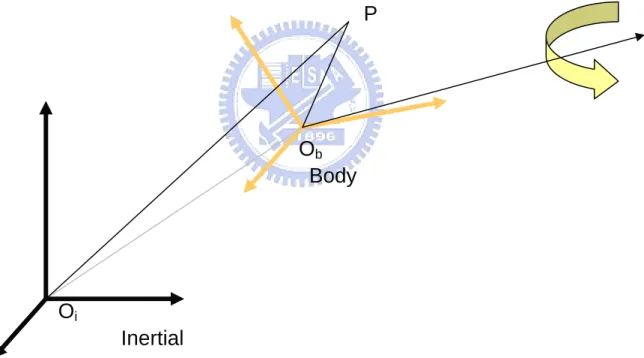
(19) CHAPTER 2 THEORY AND ALGORITHM 2.1 Motion of Rigid Body in Space Fig.2.1.1 shows motion of point P in the space between inertial frame and body frame. Oi is the origin point of inertial frame and it is centroid of the earth. Ob is the origin point of body frame and it is centroid of aircraft. Equ.1 had been derived and it is used to explain acceleration of point P between inertial frame and body frame.. P. Ob Body. Oi Inertial Fig. 2.1.1 Relation Motion between Inertial frame and Body frame. v v v v v v v v v v a = α × r + ao + ω × (ω × r ) + 2ω × r& + &r&. (2.1). where. v a. : Acceleration of point P, 5.

(20) v ao. : Acceleration of Ob,. α. v. : Angular acceleration of the body relative to inertial frame,. ω. v. : Angular rate of the body relative to inertial frame,. v r. : Location of point P relative to body frame,. v r&. : Velocity of point P relative to body frame,. &rv&. : Acceleration of point P related to body frame. v v If the point P is fixed in the body frame and it is an accelerometer on the IMU, &r& , r& ,. v v 2ω × r& must be zero and acceleration of the point is given by:. (. v v v v v v v a b = α b × r b + a0b + ω b × ω b × r b. ). (2.2). where,. v ab. : Acceleration of point P, representation in body frame,. v a0b. : Acceleration of Ob, representation in body frame,. v. : Angular acceleration of the body relative to inertial frame, representation. αb in body frame,. v. ωb. : Angular rate of the body relative to inertial frame, representation in body. frame,. 6.

(21) 2.2 Location of accelerometers and Dynamic system v Putting an accelerometer at the point P and η is the sensing direction of this accelerometer. Output of the accelerometer can be written as the form (2.3).. v v A =η b ⋅ ab v v v v v v = η b ⋅ α b × r b + η b ⋅ a0b + η b ⋅ v v v v v v = α b ⋅ r b ×η b + η b ⋅ a0b + η b ⋅. ( (. ) ). (ωv × (ωv (ωv × (ωv b. b. v ×rb v b ×rb. b. )) )). (2.3). Because of there are six degrees of freedom, six accelerometers must be required at least.. Six outputs of accelerometers can be constructed by matrix form.. Formula (2.5). v presents those on the body. Conveniently in use, J substitutes the relation between η v and r as shown in forming (2.4).. ( ( ( ( ( (. ⎡ rv b ×ηv b ⎢ v1b v1b ⎢ r2 ×η 2 ⎢ rv b ×ηv b J ≡ ⎢ v3b v3b ⎢ r4 ×η 4 ⎢ vb vb ⎢ rv5 ×ηv5 ⎢⎣ r6b ×η 6b. ) ) ) ) ) ). T. T T T T T. (ηv (ηv (ηv (ηv (ηv (ηv. b 1 b 2 b 3 b 4 b 5 b 6. ) ) ) ) ) ). ⎤ ⎥ T ⎥ T⎥ ⎥ T ⎥ T⎥ ⎥ T ⎥⎦. T. (2.4). 7.

(22) ( ( ( ( ( (. ⎡ ηv b ⎡ A1 ⎤ ⎢ v1b ⎢A ⎥ ⎢ η2 ⎢ 2⎥ v b ⎢A 3 ⎥ ⎡α ⎤ ⎢ ηv3b = ⋅ J ⎢ ⎥ ⎢ vb ⎥ + ⎢ vb A 4 ⎣ a0 ⎦ ⎢ η 4 ⎢ ⎥ ⎢ vb ⎢A 5 ⎥ ⎢ ηv5 ⎢ ⎥ ⎢⎣ η 6b ⎣⎢ A 6 ⎦⎥. ) ) ) ) ) ). T T T T T T. (ωv (ωv (ωv v ⋅ (ω v ⋅ (ω v ⋅ (ω ⋅ ⋅ ⋅. (ωv (ωv (ωv v × (ω v × (ω v × (ω. × b × b × b. b b b. v × r1b v b × r2b v b × r3b v b × r4b v b × r5b v b × r6b b. ))⎤⎥ ))⎥ ))⎥⎥ ))⎥ ))⎥⎥ ))⎥⎦. (2.5). Formula (2.6) shows the relations between output signals of each accelerometer and dynamic properties of the body in motion and includes linear acceleration of aircraft, angular rate and angular acceleration that they are all represented in the rotation frame. There is an important issue with matrix J in Eq.2.6.. In order to estimate angular. acceleration and linear acceleration from (2.6), matrix J must be invertible. In other words, rank of J must be full rank. Formula (2.7) shows the “governing equation” in our model (IMU).. Formula (2.8) presents the system output for observer to use. Formula. (2.7) is an unstable system and there is white noise in practical application, so state estimation (observer) must be used to observe the real state without this noise. This question is taken up in the next section.. ( ( ( ( ( (. v ⎡ A1 ⎤ ⎡ η1b ⎢A ⎥ ⎢ v b ⎢ 2 ⎥ ⎢ η2 vb ⎡α ⎤ -1 ⎢ A 3 ⎥ ⎢ ηv3b ⎢ v b ⎥ = J ⋅ (⎢ ⎥ - ⎢ v b ⎣ a0 ⎦ ⎢A 4 ⎥ ⎢ η 4 ⎢ A 5 ⎥ ⎢ ηv b ⎢ ⎥ ⎢ v5b ⎣⎢ A 6 ⎦⎥ ⎢⎣ η 6. ) ) ) ) ) ). T T T T T T. (ωv (ωv (ωv v ⋅ (ω v ⋅ (ω v ⋅ (ω ⋅ ⋅ ⋅. (ωv (ωv (ωv v × (ω v × (ω v × (ω. × b × b ×. b. b b b. v × r1b v b × r2b v b × r3b v b × r4b v b × r5b v b × r6b. b. ))⎤⎥ ))⎥ ))⎥⎥) ))⎥ ))⎥⎥ ))⎥⎦. 8. (2.6).

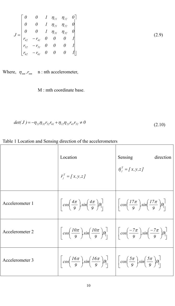
(23) ( ( ( ( ( (. v ⎡ A1 ⎤ ⎡ η1b ⎢A ⎥ ⎢ v b ⎢ 2 ⎥ ⎢ η2 ⎢ A ⎥ ⎢ ηv b v α b = J -1 (1 : 3,:) ⋅ ( ⎢ 3 ⎥ - ⎢ v3b ⎢A 4 ⎥ ⎢ η 4 ⎢ A 5 ⎥ ⎢ ηv b ⎢ ⎥ ⎢ v5b ⎣⎢A 6 ⎦⎥ ⎢⎣ η 6. [ ]. ( ( (. vb vb ⎡A 7 ⎤ ⎡ r7 ×η 7 ⎢ A ⎥ = ⎢ rv b ×ηv b ⎢ 8 ⎥ ⎢ v8 v8 ⎢⎣ A 9 ⎥⎦ ⎢⎢ r9b ×η 9b ⎣. ) ) ). T T T. T T T T T T. (ωv (ωv (ωv v ⋅ (ω v ⋅ (ω v ⋅ (ω ⋅ ⋅ ⋅. (ωv (ωv (ωv v × (ω v × (ω v × (ω. × b × b ×. b. b b b. v × r1b v b × r2b v b × r3b v b × r4b v b × r5b v b × r6b. b. ( ( ( ( ( (. ⎛ ⎡ A1 ⎤ ⎡ ηv b 1 ⎜ ⎢A ⎥ ⎢ v b ⎜ T 2 ⎢η ⎤ ⎜ ⎢ ⎥ ⎢ v2b ⎢A 3 ⎥ η T⎥ -1 ⎜ ⎥ ⋅ J ⋅ ⎜ ⎢ ⎥ - ⎢ v3b T⎥ ⎢A 4 ⎥ ⎢ η 4 ⎜ ⎢ v ⎦⎥ ⎜ ⎢ A 5 ⎥ ⎢ η 5b ⎜ ⎢⎢ A ⎥⎥ ⎢ v b ⎝ ⎣ 6 ⎦ ⎣ η6. (ηv ) (ηv ) (ηv ) b 7 b 8 b 9. ) ) ) ) ) ). ) ) ) ) ) ). T T T T T T. ( ( ( ( ( (. ))⎤⎥ ))⎥ ))⎥⎥) ))⎥ ))⎥⎥ ))⎥⎦. v ⋅ ωb × v ⋅ ωb × v ⋅ ωb × v ⋅ ωb × v ⋅ ωb × v ⋅ ωb ×. (2.7). (ωv (ωv (ωv (ωv (ωv (ωv. v × r1b v b × r2b v b × r3b v b × r4b v b × r5b v b × r6b. b. ))⎤⎥ ⎞⎟ ))⎥ ⎟⎟ ⎡(ηv ) ⋅ (ωv × (ωv ))⎥⎥ ⎟ + ⎢⎢(ηv ) ⋅ (ωv × (ωv ))⎥ ⎟⎟ ⎢(ηv ) ⋅ (ωv × (ωv ))⎥⎥ ⎟ ⎣⎢ ))⎥⎦ ⎟⎠ b T 7 b T 8 b T 9. b. b. b. v × r7b v b × r8b v b × r9b. b. ))⎤⎥ ))⎥ ))⎥⎦⎥. (2.8). In order to ensure matrix J invertible, designing the relation between location and sensing direction becomes an important issue. One way we used is that putting nine accelerometers in the same circular on the flat, Fig. 2 illustrates the location and sensing direction about all accelerometers and Table 1 shows these parameters. Location and sensing direction of the first three and 7th, 8th accelerometers sense the tangential acceleration, the 4th to 6th accelerometers sense acceleration of Z-axis only and 9th accelerometer sense the centripetal acceleration. Matrix J can be rewritten as (2.9) and the determinant of matrix J is not zero as shown in formula (2.10).. 9.

(24) ⎡0 ⎢0 ⎢ ⎢0 J =⎢ ⎢r42 ⎢r52 ⎢ ⎣⎢ r62. 1 η11 η 12 1 η 21 η 22. 0 0 0 − r41 − r51. 1 η 31 η 32 0 0 0 0 0 0. − r61 0. Where, η nm ,rnm. 0. 0. 0⎤ 0 ⎥⎥ 0⎥ ⎥ 1⎥ 1⎥ ⎥ 1⎦⎥. (2.9). n : nth accelerometer,. M : mth coordinate base.. det( J ) = −η 21η 32 r52 r61 + η 12η 21 r41 r52 ≠ 0. (2.10). Table 1 Location and Sensing direction of the accelerometers Sensing. Location. direction. v. η Tj = [ x , y , z ]. v r jT = [ x , y , z ]. Accelerometer 1. ⎡ ⎛ 4π ⎞ ⎛ 4π ⎞ ⎤ ⎢cos⎜ 9 ⎟ , sin⎜ 9 ⎟ ,0 ⎥ ⎠ ⎝ ⎠ ⎦ ⎣ ⎝. ⎡ ⎛ 17π ⎞ ⎛ 17π ⎞ ⎤ ⎢cos⎜ 9 ⎟ , sin⎜ 9 ⎟ ,0 ⎥ ⎠ ⎝ ⎠ ⎦ ⎣ ⎝. Accelerometer 2. ⎡ ⎛ 10π ⎞ ⎛ 10π ⎞ ⎤ ⎢cos⎜ 9 ⎟ , sin⎜ 9 ⎟ ,0 ⎥ ⎠ ⎝ ⎠ ⎦ ⎣ ⎝. ⎡ ⎛ − 7π ⎞ ⎛ − 7π ⎞ ⎤ ⎢cos⎜ 9 ⎟ , sin⎜ 9 ⎟ ,0 ⎥ ⎠ ⎝ ⎠ ⎦ ⎣ ⎝. Accelerometer 3. ⎡ ⎛ 16π ⎞ ⎛ 16π ⎞ ⎤ ⎢cos⎜ 9 ⎟ , sin⎜ 9 ⎟ ,0 ⎥ ⎠ ⎝ ⎠ ⎦ ⎣ ⎝. ⎡ ⎛ 5π ⎞ ⎛ 5π ⎞ ⎤ ⎢cos⎜ 9 ⎟ , sin⎜ 9 ⎟ ,0 ⎥ ⎠ ⎝ ⎠ ⎦ ⎣ ⎝. 10.

(25) Accelerometer 4. ⎡ ⎛ 2π ⎞ ⎛ 2π ⎞ ⎤ ⎢cos⎜ 9 ⎟ , sin⎜ 9 ⎟ ,0 ⎥ ⎠ ⎝ ⎠ ⎦ ⎣ ⎝. [0 ,0 ,1]. Accelerometer 5. ⎡ ⎛ 8π ⎞ ⎛ 8π ⎞ ⎤ ⎢cos⎜ 9 ⎟ , sin⎜ 9 ⎟ ,0 ⎥ ⎠ ⎝ ⎠ ⎦ ⎣ ⎝. [0 ,0 ,1]. Accelerometer 6. ⎡ ⎛ 14π ⎞ ⎛ 14π ⎞ ⎤ ⎢cos⎜ 9 ⎟ , sin⎜ 9 ⎟ ,0 ⎥ ⎠ ⎝ ⎠ ⎦ ⎣ ⎝. [0 ,0 ,1]. Accelerometer 7. ⎡ ⎛ 6π ⎞ ⎛ 6π ⎞ ⎤ ⎢cos⎜ 9 ⎟ , sin⎜ 9 ⎟ ,0 ⎥ ⎠ ⎝ ⎠ ⎦ ⎣ ⎝. ⎡ ⎛ 7π ⎞ ⎛ 7π ⎞ ⎤ ⎢cos⎜ 6 ⎟ , sin⎜ 6 ⎟ ,0 ⎥ ⎣ ⎝ ⎠ ⎝ ⎠ ⎦. Accelerometer 8. ⎡ ⎛ 12π ⎞ ⎛ 12π ⎞ ⎤ ⎢cos⎜ 9 ⎟ , sin⎜ 9 ⎟ ,0 ⎥ ⎠ ⎝ ⎠ ⎦ ⎣ ⎝. ⎡ ⎛ −π ⎞ ⎛ −π ⎞ ⎤ ⎢cos⎜ 6 ⎟ , sin⎜ 6 ⎟ ,0 ⎥ ⎠ ⎝ ⎠ ⎦ ⎣ ⎝. Accelerometer 9. [1,0 ,0 ]. [1,0 ,0 ]. 11.

(26) 1. 7. 4 Y. 5. X. 9. Z 2 3 8. 6. Fig.2.2.1 Location and Sensing direction of the nine accelerometers. According to the above parameters of accelerometers, governing equation (2.7) and output equation (2.8) can be rewritten as (2.11) (2.12).. ⎡ A1 ⎤ ⎢A ⎥ b ⎢ 2⎥ ⎡ ⎡ω& 1 ⎤ ⎢A 3 ⎥ ⎢ ⎢ b⎥ −1 & ( ) = ⋅ J 1 : 3 , : ω ⎢ ⎥+⎢ 2 ⎢ ⎥ ⎢A 4 ⎥ ⎢a ω b ⎢ω& 3b ⎥ ⎣ ⎦ ⎢A 5 ⎥ ⎣ 1 1 ⎢ ⎥ ⎢⎣A 6 ⎥⎦. − ω 2bω3b. ⎤ ⎥ ωω ⎥ 2 2 2 + a 2 ω 2b + (a1 + a 2 ) ω 3b + a3ω1bω 2b ⎥⎦. ( ). b 1. ( ). ⎡ A1 ⎤ ⎢A ⎥ ⎡ ωb 2 + ωb ⎢ 2⎥ ⎡ A7 ⎤ 1 3 ⎢ A ⎥ = ACoef 1 ⋅ ⎢ A 3 ⎥ + ACoef 2 ⋅ ⎢ ω b 2 + ω b ⎢ 2 ⎢ ⎥ 3 ⎢ 7⎥ A4 ⎥ b b ⎢ ⎢ ⎢⎣ A7 ⎥⎦ ⎢⎣ ω1 ω3 ⎢A 5 ⎥ ⎢ ⎥ ⎢⎣A 6 ⎥⎦. ( ) ( ) ⎤⎥ ( ) ( )⎥. 12. b 3. ( ). (2.11). 2. 2. ⎥ ⎥⎦. (2.12).

(27) Formula (2.11) and (2.12) present the dynamic system in the continuous time domain. In order to program the above system, ω& j can be discretize by ω j (k + 1) ､ ω j (k ) and dt as formula (2.13).. Formula (2.14) and (2.15) show the discrete system from (2.11) and. (2.12) by (2.13).. ω& j =. ω j (k + 1) − ω j (k ) dt. (2.13). ⎡ A1 (k )⎤ ⎢A (k )⎥ b ⎢ 2 ⎥ ⎡ω1 (k + 1)⎤ ⎢ A 3 (k )⎥ ⎢ b ⎥ −1 ( ) ( ) + = ⋅ ω k 1 J 1 : 3 , : ⎢ ⎥ ⋅ dt 2 ⎢ ⎥ A 4 (k )⎥ b ⎢ ⎢ω3 (k + 1)⎥ ⎣ ⎦ ⎢ A 5 (k )⎥ ⎢ ⎥ ⎢⎣A 6 (k )⎥⎦. ⎡ ⎤ ⎡ω1b (k )⎤ − ω 2b (k )ω3b (k ) ⎢ ⎥ ⎢ ⎥ +⎢ ⋅ dt + ⎢ω 2b (k )⎥ ω1b (k )ω 3b (k ) ⎥ ⎢a1 ω1b (k ) 2 + a2 ω 2b (k ) 2 + (a1 + a2 ) ω3b (k ) 2 + a3ω1b (k )ω 2b (k )⎥ ⎢ω3b (k )⎥ ⎣ ⎦ ⎣ ⎦. (. ). (. ). (. ). (2.14) ⎡ A1 (k )⎤ ⎢A (k )⎥ ⎡ ω b (k ) 2 + ω b (k ) 2 ⎤ ⎢ 2 ⎥ ⎡ A7 (k )⎤ 1 3 ⎢ A (k )⎥ = ACoef 1 ⋅ ⎢ A 3 (k )⎥ + ACoef 2 ⋅ ⎢ ω b (k ) 2 + ω b (k ) 2 ⎥ ⎥ ⎢ 2 ⎢ ⎥ 3 ⎢ 8 ⎥ A 4 (k )⎥ b b ⎥ ⎢ ⎢ ⎢⎣ A9 (k )⎥⎦ ⎢⎣ ω1 (k )ω3 (k ) ⎥⎦ ⎢ A 5 (k )⎥ ⎢ ⎥ ⎢⎣A 6 (k )⎥⎦. ( (. 2.3 Kalman filter 2.3.1 The Extended Kalman Filter. 13. ) ( ) (. ) ). (2.15).

(28) Consider the nonlinear system with dynamics x(k + 1) = f [k. x(k )] + v(k ). (2.16). where, for simplicity, it is assumed that there is no control, and the noise is assumed additive, zero mean, and white Gaussian distribution. E[v(k )] = 0. ′ E ⎡ v(k )v( j) ⎤ = R(k )δ kj ⎥⎦ ⎢⎣. (2.17). The measurement is z (k ) = h[k. x(k )] + ω (k ). (2.18). Where the measurement noise is additive, zero mean, and white ′ E[ω (k )] = 0 E ⎡ω (k )ω ( j ) ⎤ = R(k )δ kj ⎥⎦ ⎢⎣. (2.19). Because of this is a nonlinear system, the system need to be linearization. Formula (2.20) uses Taylor series expansion to linearize system and measurement for obtaining the optima estimation of the system. x (k + 1) ⎤ ⎡ 1 nx ′ = f ⎢k, ˆx (k | k ) + f x (k )[x (k ) - ˆx (k | k )] + ∑ e i [x (k ) - ˆx (k | k )] f xxi (k )[x (k ) - ˆx (k | k )]⎥ 2 i =1 ⎦ ⎣ + HOT + v(k ) (2.20). where 14.

(29) : i th Cartesian basis vector,. ei. f x (k ) ≡. ′ ∂f ⎡ ′ ≡ ∇ x f (k, x ) ⎤ | x = ˆx (k|k ) ⎥⎦ ∂x ⎢⎣. : the Jacobian of vector f,. ∂ 2f i ⎡ ′ ′ ≡ ∇ x ∇ x f i (k, x ) ⎤ | x = xˆ (k|k ) ⎥⎦ ∂x 2 ⎣⎢. : the Hessian of vector f,. f xxi (k ) ≡. HOT. : higher-order terms.. State prediction. The predicted state to time k + 1 from time k is obtained by taking the expectation of (2.20) neglecting HOT.. ˆx (k + 1 | k ) = f [k, ˆx (k | k )] +. [. ]. 1 nx e i tr f xxi P(k | k ) ∑ 2 i=1. (2.21). And prediction covariance is: ′ P(k + 1 | k ) = f x (k )P(k | k )f x (k ) +. [. (2.22). ]. 1 nx nx ′ e i e j tr f xxi (k )P(k | k )f xxj (k )P(k | k ) + Q(k ) ∑∑ 2 i=1 j=1. Measurement prediction. Similarly, the predicted measurement is, for the second-order filter. [. ]. 1 nz ˆz(k + 1 | k ) = h[k + 1, ˆx(k + 1 | k )] + ∑ ei tr h ixx (k + 1)P(k + 1 | k ) 2 i=1. 15. (2.23).

(30) The measurement prediction covariance or innovation covariance or residual covariance--really MSE matrix—is S(k + 1) ′ = h x (k + 1)P(k + 1 | k )h x (k + 1) +. (2.24). [. ]. 1 nx nx ′ j (k + 1)P(k + 1 | k ) + R (k + 1) e i e j tr h ixx (k + 1)P(k + 1 | k )h xx ∑∑ 2 i =1 j=1. Filter gain -1 ′ W (k + 1) = P(k + 1)h x (k + 1) S(k + 1). (2.25). Update. The state estimate updated is. ˆx (k + 1 | k + 1) = ˆx (k + 1 | k ) + W (k + 1)ν(k + 1). (2.26). and state covariance updated is. ′ P(k + 1 | k + 1) = P(k + 1 | k ) - W (k + 1)S(k + 1)W(k + 1). (2.27). The optima estimation will obtain from the above calculating repeatedly.. Using the first-order extended Kalman filter, the higher-order term and the Hessian of f, and h will be neglected. For simplify to use the first order extended Kalman filter, Table 2 is presented the flow chat included state prediction and state update.. 16.

(31) Known input Evolution. (control or. of the system. Sensor. Estimation. State covariance. (true state). motion). of the state. computation. State at tk. Input at tk. State estimate at tk. State covariance at tk. X(k). U(k). xˆ (k|k). P(k|k). Evaluation of Jacobians & Hessian. ∂f ( k ) |x = ˆx ( k |k ) ∂x ∂2 f i( k ) |x = ˆx ( k |k ) F xxi ( k ) = ∂x 2 ∂ h( k + 1 ) |x = ˆx ( k |k + 1 ) H x( k + 1) = ∂x ∂ 2hi( k + 1 ) |x = ˆx ( k |k + 1 ) H xxi ( k + 1 ) = ∂x 2 Fx ( k ) =. Transition U(k). State prediction. x( k + 1 ) =. ˆx ( k + 1 | k ) = f [ k , ˆx ( k | k ), u ( k )]. f [ k , x( k ), u( k )] + υ( k ). State prediction covariance. P( k + 1| k ) = Fx( k )P( k | k )Fx( k )' + Q( k ). Measurement prediction. Zˆ (k + 1 | k ) = h[k + 1, xˆ (k + 1 | k )]. Residual covariance. S( k +1) = Hx( k + 1)P( k +1| k )Hx( k +1)' + R( k ). Measurement residual. (k + 1 ) = z (k + 1 − ˆz (k + 1 | k ). ν. ) Filter gain. W (k + 1) = P(k + 1 | k ) H (k + 1)' S (k + 1) −1. Measurement at tk+1 W(k+1). z( k + 1 ) = h [ k + 1, x( k + 1 )] + w( k + 1 ). Update state estimate. xˆ (k + 1 | k + 1) = xˆ (k + 1 | k ) + W (k + 1)ν (k + 1). Table 2 Flow chart of first order Extended Kalman filter. 17. Update state covariance P (k + 1 | k + 1) = P (k + 1 | k ) − W (k + 1) S ( k + 1)W (k + 1)'.

(32) 2.3.2 The Iterated Extended Kalman Filter A modified state updating approach can be obtained by an iterative procedure as follows.. [. ]. H i ≡ h x k + 1, ˆx i (k + 1 | k + 1). (2.28). P i (k + 1 | k + 1) = P(k + 1 | k ) −1. ′ ′ ′ − P(k + 1 | k )H (k + 1) ⎡H i (k + 1)P(k + 1 | k )H i (k + 1) + R (k + 1)⎤ H i (k + 1)P(k + 1 | k ) ⎢⎣ ⎥⎦ i. (2.29) ˆx i +1 (k + 1 | k + 1) = ˆx i (k + 1 | k + 1). {. [. ]}. −1 ′ + P i (k + 1 | k + 1)H i (k + 1) R (k + 1) z(k + 1) − h k + 1, ˆx i (k + 1 | k + 1). [. ]. −1 − P i (k + 1 | k + 1)P(k + 1 | k ) ˆx i (k + 1 | k + 1) − ˆx (k + 1 | k ). (2.30). Starting the iteration for i = 0 with. ˆx 0 (k + 1 | k + 1 ) ≡ ˆx (k + 1 | k ) causes the last term in (2.30) to be zero and yields after the first iteration ˆx 1 (k + 1 | k + 1) , that is, the same as the first-order (no iterated) EKF.. Overview of the Iteration Sequence. 18.

(33) For i=(0:N-1). (2.28). (2.29). (2.30). For i=N. (2.30). with N decided either a prior or based on a convergence criterion.. Through the above procedure to calculate angular rate and linear acceleration represented in body frame repeatedly, we can obtain the optima estimation at time k + 1 .. 2.4 Orthogonal Transfer Matrix In order to consider the angular rate and linear represented in inertial frame, the orthogonal matrix should be used to transfer the representation to another base which interests us. Formula (2.31) shows the relation between two different bases.. X b = AX i. (2.31). Where. X b : Representation in body frame,. 19.

(34) A. : Orthogonal transfer matrix,. Xi. : Representation in inertial frame. The Euler angles θ , φ and ϕ are an orthogonal transform to transfer the quantities. in the rotation frame into those in the inertial frame.. Fig.2.4.1 shows the sequence that is started by rotating the initial system of axes, XYZ, by an angle φ counterclockwise about the Z axis, and the resultant coordinate system is labeled the ξηζ axes.. In the second step, the intermediate axes, ξηζ , are. rotated about the η axis counterclockwise by the angle θ to produce another intermediate set, the ξ ′η ′ζ ′ axes.. Finally, the ξ ′η ′ζ ′ axes are rotated counterclockwise. by an angle ϕ about the ζ ′ axis to produce the desired X′Y′Z′ system of axes. Follow the above three separate rotation is called Y-Convention. Formulas (2.32) to (2.34) show the relation like (2.31) in the three rotations. Formula (2.35) shows the result of the three separate rotations, and A is the orthogonal transfer matrix defined in formula (2.31).. Formula (2.36) shows inverse A to transfer representation from the. body frame to the inertial frame.. ξ = DX i. (2.32). ξ ′ = Cξ. (2.33). X b = Bξ ′. (2.34). 20.

(35) A = BCD ⎡ cos ϕ = ⎢⎢- sin ϕ ⎢⎣ 0. sin ϕ cos ϕ 0. 0⎤ ⎡cos θ 0 − sin θ ⎤ ⎡ cos φ 0⎥⎥ ⎢⎢ 0 1 0 ⎥⎥ ⎢⎢− sin φ 1⎥⎦ ⎢⎣ sin θ 0 cos θ ⎥⎦ ⎢⎣ 0. sin φ cos φ 0. 0⎤ 0⎥⎥ 1⎥⎦ (2.35). X i = A -1X b = A′X b A′ = D′C′B′ ⎡cos ϕ - sin ϕ 0 ⎤ ⎡ cos θ 0 sin θ ⎤ ⎡cos φ - sin φ 0 ⎤ 1 0 ⎥⎥ ⎢⎢ sin φ cos φ 0 ⎥⎥ = ⎢⎢ sin ϕ cos ϕ 0 ⎥⎥ ⎢⎢ 0 ⎢⎣ 0 0 1⎥⎦ 0 1⎥⎦ ⎢⎣- sin θ 0 cos θ ⎥⎦ ⎢⎣ 0 ⎡- sin φ sin ϕ + cos θ cos φ cos ϕ − sin φ cos ϕ − cos θ sin ϕ cos φ cos φ cos ϕ − cos θ sin ϕ sin φ = ⎢⎢ cos φ sin ϕ + cos θ cos ϕ sin φ ⎢⎣ sinθ cos ϕ sinθ sin ϕ. Z. Z′. (2.36) cos sinθ ⎤ sin sinθ ⎥⎥ cos θ ⎥⎦. Z. Y′ η. =. Y. X. X′. Y. Z. X. Z. ξ. Z′. η′. ς′. +. Y′. η′. η. Y. +. Y. ξ X. X. ξ′. ξ′. X′. Fig.2.4.1 Eular’ angle. It is often convenient to express the angular rate vector in terms of Euler angles and 21.

(36) their time derivatives as (2.37). In consequence of the vector property of infinitesimal rotations, the vector Euler angles time derivatives can be obtained as the sum of the three separate angular rate vectors and ω .. The angle θ must avoid being zero. carefully, or make the element in the (2.37) singular.. ⎡ − cos ϕ ⎡φ& ⎤ ⎢ ⎢ & ⎥ ⎢ sin θ ⎢θ ⎥ = ⎢ sin ϕ ⎢ϕ& ⎥ ⎢ cosθ cos ϕ ⎣ ⎦ ⎣⎢ sin θ. sin ϕ sin θ cos ϕ − cosθ sin ϕ sin θ. ⎤ 0⎥ ⎡ω x ⎤ 0⎥ ⎢⎢ω y ⎥⎥ ⎥ 1⎥ ⎢⎣ω z ⎥⎦ ⎦⎥. (2.37). 2.5 Flow chart Fig.2.5.1 shows the procedure how to use these accelerometers to obtain all information in the body frame or inertial frame.. A1~A6 A7~A9. System(algorithm). Iterate EKF ω b ,ab. ω i ,ai. Eular angle. ϕ& ,θ& ,φ&. ϕ ,θ ,φ Fig.2.5.1 The flow chart of all algorithms. 22.

(37) CHAPTER 3 SIMULATION AND PRELIMINARY TEST The algorithm introduced in Chapter 2 will be proved by simulating with Matlab package.. In this proof, consider about the random noise with accelerometer output will. be measured from static-tested of an accelerometer on a stage. In order to make sure that the experiments are accurate, we test the response of one axis with one accelerometer at first. The structure of test will be presented in section 3.2. Section 3.3 shows that how to simulate the motion and define the suitable accelerometer output signal. Section 3.4 shows that preliminary tested from an accelerometer in the above motion we defined. Section 3.5 shows Matlab simulation to ensure the algorithm we derived in Chapter 2.. 3.1 Test structure In order to get pure sine wave acceleration, the function generator employs to provide PWM servo amplifiers command and those drives the DC motor on the stage.. The stage. is driven by Dc motor and generates a sinusoidal acceleration which is less than 1g. And the output of accelerometer (ADXL105) is set to a nominal scale factor of 250 mV/g. However, in order to reduce SNR and increase accuracy, the circuits used to amplify output voltage must be needed.. Information of encoder of the DC motor is measured by motion card (ADLINK PCI-8133) and the accelerometer output signals are measured by DAQ card (ADLINK PCI-9114). Then, we need 2 consecutive integral operations to obtained displacement of stage and compare those with encoder information. Fig.3.2.1 shows the block diagram of the test system. 23.

(38) Function generator. PWM servo amplifiers. Stage (ILS100CC). Motion card (ADLINK PCI-8133) Compare position error. DAQ card (ADLINK PCI-9114) Accelerometer (ADXL105) output signal. ∫∫ dtdt. Fig.3.2.1 Structure of uni-axis test. 3.2 Generate Motion Pure sine wave assists us to analysis the signal easily. It is different between the input commands of the DC motor from the output of accelerometer, because it loses the energy on stage. In order to make sure that the signal is the pure sin wave, tuning the frequency of the function generator until the differential data of encoder twice to be like the pure sinusoidal response. Fig.3.3.1 to Fig.3.3.3 shows the result of these procedures.. Fig.3.3.1 1HZ sin wave of function generator 24.

(39) Fig.3.3.2 11HZ sin wave of function generator. Fig.3.3.3 18HZ sin wave of function generator. We can obtain the result that we increase the frequency of the function generator and the acceleration becomes pure sine wave. If we increase the frequency of the function generator over than about 20HZ, we will get the smaller amplitude of the acceleration than before.. Finally, 18HZ of the function generator is employed to be the input command in. this one axis tested.. 3.3 One Axis Tested 25.

(40) In the above condition, the acceleration output will be measured by DAQ card. Fig.3.4.1 shows the acceleration output, the data which is obtained by integrating the output of accelerometer once or twice, and we compare those with the information of the encoder.. The accumulation of integral error can be indicated clearly as shown in. Fig.3.4.1.. The source of this error is the drift of the accelerometer output and the. vibration of optical table. This question is taken up in the chapter.5.. compare encoder and measurement. mm. 10 encoder accelerometer. 5 0 -5. 0. 0.5. 1. 1.5. 2. 1.3. 1.4. 2.5. 3. 3.5. 4. 4.5. 5. 1.5 encoder accelerometer. mm. 1 0.5 0 1. mm/s. 20. 1.1. 1.2. 1.5. 1.6. 1.7. 1.8. 1.9. 2. velocity from accelerometer. 0 -20 1. 1.2. 1.3. 1.4. 1.5. 1.6. 1.7. 1.8. 1.9. 2. acceleration from accelerometer. 2000 mm/s 2. 1.1. 0 -2000 1. 1.1. 1.2. 1.3. 1.4. 1.5. 1.6. 1.7. 1.8. 1.9. 2. Fig.3.4.1 Compare encoder and accelerometer output. The sampling rate of encoder is 500 HZ and the sampling rate of DAQ card is 2000 HZ. When the DC motor is static, the standard deviation is 21.9416 mm/s2.. The. amplify scale is 1000/39, the operator voltage is 0V and 5V and the accelerometer output scale is 250 mV/g, so acceleration must be smaller than 0.39g (3900mm/ s2) with 26.

(41) these conditions. Formula 3.1 shows the result.. (5V/2)*(39/1000)/(0.25)=0.39. (3.1). 3.4 Simulation and Resolution We define the path of the angular acceleration of the Euler’s angles and linear accelerations in the inertial frame as formula(3.2).. We assume that sampling rate of DAQ. card is 1000HZ, l=50mm and the standard deviation is 25mm/ s2.. ⎡φ& ⎤ ⎡2 × π/3⎤ ⎢ &⎥ ⎢ ⎥ (rad / s ) ⎢θ ⎥ = ⎢2 × π/3⎥ ⎢ϕ& ⎥ ⎢⎣2 × π/3⎥⎦ ⎣ ⎦ ⎡A x ⎤ ⎡2000 × sin(2 × pi ×18 × t)⎤ ⎢ A ⎥ = ⎢2000 × sin(2 × pi ×18 × t)⎥ mm/s 2 ⎢ y⎥ ⎢ ⎥ ⎢⎣ A z ⎥⎦ ⎢⎣2000 × sin(2 × pi ×18 × t)⎥⎦. (. ) (3.2). Fig.3.5.1 shows the state of the algorithm we derived and Fig.3.5.2 shows the angular rate in the inertial frame.. 27.

(42) w1 in rotated frame. w2 in rotated frame. 3. 3 measured real. 2. 1 rad/s. rad/s. 1 0. 0. -1. -1. -2. -2. -3. measured real. 2. 0. 1. 2. 3. 4. -3. 5. 0. 1. 2. 3. 4. 5. w3 in rotated frame 5 measured real. 4. rad/s. 3 2 1 0 -1. 0. 1. 2. 3. 4. 5. Fig.3.5.1 angular rate representation in Body frame. w1 in Inertial frame. w2 in Inertial frame. 3. 3 measured real. 2. 1 rad/s. rad/s. 1 0. 0. -1. -1. -2. -2. -3. measured real. 2. 0. 1. 2. 3. 4. -3. 5. 0. 1. 2. 3. 4. 5. w3 in Inertial frame 5 measured real. 4. rad/s. 3 2 1 0 -1. 0. 1. 2. 3. 4. 5. Fig.3.5.2 angular rate representation in the Inertial frame. Fig.3.5.3 shows the Euler’s angular rate and Fig.3.5.4 shows the Euler’s angle. There is pulse at 1.5, 3 and 4 seconds, because the matrix in formula (2.37) is singular.. 28.

(43) wf ife in euler anlge. wtheta in euler angle. 4000. 3 measured real. 2000. 1 rad/s. rad/s. 0 -2000. 0. -4000. -1. -6000. -2. -8000. measured real. 2. 0. 1. 2. 3. 4. -3. 5. 0. 1. 2. 3. 4. 5. wphi in euler angle 4000 measured real. 2000. rad/s. 0 -2000 -4000 -6000 -8000. 0. 1. 2. 3. 4. 5. Fig.3.5.3 angular rate of Euler angles. fife in euler anlge. theta in euler angle. 15. 12 measured real. 10. measured real. 10 8 rad. rad. 5 6. 0 4 -5 -10. 2 0. 1. 2. 3. 4. 0. 5. 0. 1. 2. 3. 4. 5. phi in euler angle 15 measured real. 10. rad. 5 0 -5 -10. 0. 1. 2. 3. 4. 5. Fig.3.5.4 Euler angles. The iterative time is 40 for initial to 0.1 second and 20 for 0.1 second to 1 second. Fig.3.5.5 shows the result of iteration.. 29.

(44) w2. w1 0.5334. -2.7371 Iterative convergence. Iterative convergence 0.5332. -2.7372 0.533 -2.7373. 0.5328 0.5326. -2.7374 0.5324 -2.7375. 0. 10. 20. 30. 40. 0.5322. 50. 0. 10. 20. 30. 40. 50. w3 1.0438 Iterative convergence 1.0437 1.0436 1.0435 1.0434 1.0433 1.0432. 0. 10. 20. 30. 40. 50. Fig.3.5.5 Iterative convergence of angular rate representation in body frame. Fig.3.5.6 shows the linear accelerations in the body frame and Fig.3.5.7 shows the linear accelerations in the inertial frame.. Fr1. Fr2. 3000. 4000 measured real. 2000. measured real 2000 2. mm/s. mm/s. 2. 1000 0. 0. -1000 -2000 -2000 -3000. 0. 1. 2. 3. 4. -4000. 5. 0. 1. 2. 3. 4. Fr3 4000 measured real. mm/s. 2. 2000. 0. -2000. -4000. 0. 1. 2. 3. 4. 5. Fig.3.5.6 Linear acceleration representation in Body frame. 30. 5.

(45) F1 in Inertial frame. F2 in Inertial frame. 2000. 2000. measured real 1000. measured real. 2. mm/s. mm/s. 2. 1000. 0. -1000. 0. -1000. -2000. -2000 1. 1.2. 1.4. 1.6. 1.8. 2. 1. 1.2. 1.4. 1.6. 1.8. 2. F3 in Inertial frame 2000 measured real. mm/s. 2. 1000. 0. -1000. -2000 1. 1.2. 1.4. 1.6. 1.8. 2. Fig.3.5.7 Linear acceleration representation in Inertial frame. Resolution w1 in rotated frame. w2 in rotated frame. 0.04. 0.06 measured real. 0.02. 0.02 rad/s. rad/s. 0 -0.02 -0.04 -0.06. measured real. 0.04. 0 -0.02. 0. 50. 100. -0.04. 150. 0. 50. 100. 150. w3 in rotated frame 0.08 measured real. 0.06. rad/s. 0.04 0.02 0 -0.02. 0. 50. 100. 150. Fig.3.5.8 Angular rate in the rotation frame (R=50mm, std=0.1mm/s2) Fig.3.5.8 shows the angular rate in the rotation frame with R=50mm, stander deviation (std)=0.1mm/s2 and resolution is 12 ∘/s . We assume that the angular 31.

(46) acceleration and linear acceleration is zero, and rewrite Eq.2.3 as Eq.3.3. We can find out the relationship between resolution of accelerometer and angular rate of our algorithm shown as Eq.3.4. v v A = η b ⋅ ab v v v v v v v v v = η b ⋅ α b × r b + η b ⋅ a0b + η b ⋅ ω b × ω b × r b v v v v =η b ⋅ ωb × ωb × r b. ( (. (. ). )). (. (. )). ⇒ A ∝ rω 2. (3.3). A r. (3.4). ⇒ω ∝. 32.

(47) CHAPTER 4 TEST OF THE IMU DESIGN To verify the feasibility and reliability of the method for computing angular rate, it is necessary to perform a two-step validation procedure, i.e., the method has to yield consistent and accurate results while acquiring data both from hypothetical and experimental systems.. To check if our method is feasible for any arbitrary motion, some experiments with different configurations should be done. According to the type of Euler＇s angle (ZYZ convention), we design three different experiments and simulations.. First, Z axis in the. body frame is parallel to the axis of rotation and the other two linear motions are parallel to the inertial frame. Secondly, initial condition is changed in order to verify the observer method is practical when acceleration of gravity effect on the output of accelerometer. Thirdly, Y axis in body frame is parallel to the axis of rotation and the other two linear motions are parallel to the inertial frame.. Section 4.1 describes the procedures for these experiments with the designed motion, analog amplifier, and Butterworth filter.. Section4.2, 4.3 and 4.4 describes the first,. second and third experiment and simulation, respectively.. 4.1 Experimental procedure Basic procedure of experiment, analog low-pass amplifier, Butterworth filter and designed motion will be introduced in this section, and variation of tri-axial setup will be present in the flowing section.. 33.

(48) Basic procedure of experiment. Three different function generators output sinusoidal voltage to three different PWM servo amplifiers. stages.. These servo amplifiers output sinusoidal current to three different. Sinusoidal current excite sinusoidal acceleration on the stage and we put our IMU. on the stage to sense the sinusoidal acceleration and read the encoder information by motion card (ADLINK PCI-8133). System noise or disturbance will be generated when three stages create the sinusoidal. nominally 250mV/g.. And the acceleration output of the ADXL105 is. This scale factor is not appreciated for our applications.. An. amplifier is need to set an appreciate scale ratio and a low-pass filter is needed to filter accelerometer’s internal or circuit high-frequency noise, so analog 1-pole low-pass filter will be employed to filter those between accelerometer and DAQ card (ADLINK PCI-9114). But other high-frequency noise will be excited when data of acceleration are transferred between the output of 1-pole low-pass filter and DAQ card. The digital filter (4th order Butterworth filter) must be needed to filter this noise by computer. Let the result of digital filter be as acceleration output (A1~A9) shown as in algorithm, and physical quantities can be calculated by our observer base IMU.. To compare these. quantities and encoder’s information, and we will know our algorithm be practical or not. We will discuss every physical quantities which interest us to be practical or not in the following sections. Fig.4.1.1 and Fig.4.1.2 show the process of experiment and the flow chart of algorithm respectively.. 34.

(49) Function generator. PWM servo amplifiers. Stage(ILS100CC & RV80CC) Motion card (ADLINK PCI-8133) Accelerometer (ADXL105) output signal DAQ card (ADLINK PCI-9114) Analog amplifier. Butterworth. A1~A9. Fig.4.1.1 Experimental procedure. A1 A2 A3 A4 A5 A6 A7 A8 A9. vb f. [ ]. vi f = we f. system. v. ωb System + Kalman filter. θ& e = [θ e ]ω b v. vi vb f. ∫∫. v. ωe. vi. v ω ∫ ω = w ωb i. Fig. 4.1.2 Algorithm flow 35. p. [ ] e. θ.

(50) Route of motion. Because sinusoidal current excited sinusoidal acceleration on the stage, Eq.4.1 describes the relationship about displacement, velocity and acceleration. Fig.3.4.1 shows tendency of Eq.4.1. Accelaration = sin (2πft ) 1 1 Velocity = − cos(2πft ) + 2πf 2πf 1 1 sin (2πft ) + t Displacement = − 2 2πf (2πf ). (4.1) Low-pass analog amplifier (single pole). C. R1 R2 IN. VMID. OUT. +. Fig.4.1.3 Circuit of low-pass analog amplifier (single pole). Fig.4.1.3 presents the circuit of low-pass filter and Fig.4.1.4 shows the Bode plot of low-pass filter.. Eq.4.2 describes the gain is 5.1282 and Eq.4.3 shows the transfer function. when the cutoff frequency is 117.0257 HZ, and.. 36.

(51) 1 2ππCR R1 GAIN = − R2 R1 = 200KΩ R2 = 39KΩ. f − 3dB =. (4.2). C = 6.8 × 10− 9 F. T=. 5.128 0.00136 s + 1. (4.3). analog low pass filter 20. Magnitude (dB). 10. 0. -10. -20. Phase (deg). -30 0. -45. -90 1. 10. 2. 3. 10. 10. 4. 10. 5. 10. Frequency (rad/sec). Fig.4.1.4 Low-pass analog amplifier (single pole) Butterworth filter. Butterworth filters are characterized by a magnitude response that is maximally flat in the pass-band and monotonic overall.. Butterworth filters sacrifice roll-off steepness for. monotonic in the pass- and stop-bands. Unless the smoothness of the Butterworth filter is. 37.

(52) needed, an elliptic or Chebyshev filter can generally provide steeper roll-off characteristics with a lower filter order. Eq.4.4 shows the Z-transform and Fig.4.1.5 shows frequency response when data sampled at 2000 Hz and design a 4th-order low-pass Butterworth filter with cutoff frequency of 50 Hz.. H(Z) =. 3.12 × 10 −5 + 1.25 × 10 −4 Z −1 + 1.87 × 10 −4 Z −2 + 1.25 × 10 −4 Z −3 + 3.12 × 10 −5 Z −4 1 − 3.5897 Z −1 + 438513Z − 2 − 2.9241Z −3 − 6.6301 × 10 −1 Z − 4. (4.4). Butterworth 100. Magnitude (dB). 0 -100 -200 -300 -400. 0. 100. 200. 300. 400. 500 600 Frequency (Hz). 700. 800. 900. 1000. 0. 100. 200. 300. 400. 500 600 Frequency (Hz). 700. 800. 900. 1000. Phase (degrees). 0. -100. -200. -300. -400. Fig.4.1.5 Butterworth low-pass filter (fourth order). There is invariably a time delay between a demodulated signal and the original received signal.. The Butterworth filter parameters directly affect the length of this delay.. 4.2 Z-axis rotation with biaxial linear acceleration. 38.

(53) In this experiment, Z axis in body frame is parallel to the axis of rotation and the other two linear motions are parallel to X axis and Y axis in the inertial frame respectively. Fig.4.2.1 shows this experiment setup. Eq.4.5 presents Euler ＇ s transform in these condition. Generally speaking, whether the quantity of Z-axis in the rotation frame or in the inertial frame must be equal to the Euler＇s angle (φ + ϕ ) , and the quantities of X-axis, Y-axis and Euler＇s angle θ must be zero. But that is not exact correct in practical experiment.. We shall now look more carefully into Eq.4.5, the quantity of Z-axis must. be equal to the Euler＇s angle (φ + ϕ ) when the disturbance or noise in the Euler＇s angle θ is close to zero, and the quantity of Z-axis is equal to ϕ when the disturbance or noise in the Euler＇s angle θ is larger then a value which is over than 0.06 radian after 0.2 seconds in this experiment. understand this question.. Compared Fig.4.2.7 with Fig.4.2.8, and we can clearly Fig.4.2.2 shows accelerations which are through analog. low-pass filter and Fig.4.2.3 shows accelerations which are through analog low-pass filter and then are through digital Butterworth low-pass filter.. The curve in Fig.4.2.3 is. smoother then in Fig.4.2.2 and in Fig.4.2.3; there is invariably a time delay which is introduced in the above section. In Fig.4.2.4 and Fig.4.2.6~4.2.13, the information of encoder shown by solid line, result of estimated shown by dotted line and subtracting time delay shown by dash-dot line. The rule holds in the flowing two sections.. 39.

(54) Fig.4.2.1 Experimental set up. θ =0 ⎡cos ϕ X = ⎢⎢ sin ϕ ⎢⎣ 0 i. - sin ϕ 0⎤ ⎡ cos θ 0 sin θ ⎤ ⎡cos φ - sin φ 0⎤ 1 0 ⎥⎥ ⎢⎢ sin φ cos φ 0⎥⎥ X b cos ϕ 0⎥⎥ ⎢⎢ 0 0 1⎦⎥ 0 1⎥⎦ ⎢⎣- sin θ 0 cos θ ⎥⎦ ⎢⎣ 0 ⎡- sin φ sin ϕ + cos φ cos ϕ − sin φ cos ϕ − sin ϕ cos φ 0⎤ cos φ cos ϕ − sin ϕ sin φ 0⎥⎥ X b = ⎢⎢ cos φ sin ϕ + cos ϕ sin φ 0 0 1⎦⎥ ⎣⎢. ⎡cos(φ + ϕ ) − sin (φ + ϕ ) 0⎤ = ⎢⎢ sin (φ + ϕ ) cos(φ + ϕ ) 0⎥⎥ X b ⎢⎣ 0 0 1⎥⎦. 40. (4.5).

(55) nine accelerometer output with only r otation motion. 4. x 10. NO.1 NO.2 NO.3 NO.4 NO.5 NO.6 NO.7 NO.8 NO.9. 1. mm/s2. 0.5. 0. -0.5. -1. 0.02. 0.04. 0.06. 0.08. 0.1 sec. 0.12. 0.14. 0.16. 0.18. 0.2. Fig.4.2.2 Nine accelerometers output. nine accelerometer output with only rotation motion after filtering. 4. x 10. NO.1 NO.2 NO.3 NO.4 NO.5 NO.6 NO.7 NO.8 NO.9. 1 0.8 0.6 0.4. mm/s. 2. 0.2 0 -0.2 -0.4 -0.6 -0.8 -1. 0.02. 0.04. 0.06. 0.08. 0.1 sec. 0.12. 0.14. 0.16. Fig.4.2.3 Signals after Butterworth low-pass filter. 41. 0.18. 0.2.

(56) Fig.4.2.4 shows the angular rate which is estimated from observer and obtained from differentiating the data of encoder in the rotation frame, Fig.4.2.10 shows that those are in the inertial frame and Fig.4.2.7 shows the Euler＇s angular rate. These quantities in X-axis and Y-axis should converge to zero, and in Z-axis should be the sinusoidal wave which is according Eq.4.1.. But zero is smaller then resolution in our algorithm, these two. curves will not converge to zero. We simulate the same condition as shown in Fig.4.2.5, and angular rate don’t converge to zero in X-axis and Y-axis. Because quantity in Z-axis in the rotation frame is equal to it in the inertial frame and (φ + ϕ ) , angular displacement can be obtained by integrating from angular rate directly whether it is in the rotation or inertial frame as shown in Fig.4.2.6 and Fig.4.2.11 respectively.. Euler ＇ s angular. displacement is obtained from solving differential equation (Eq.2.37) directly and shown in Fig.4.2.9. The integral method will accumulate the error and make serious mistake when using Euler＇s transform as shown in Fig.4.2.13.. w1 in rotated frame. w2 in rotated frame. 0. rad/s. rad/s. 1.5. 1. -0.5. 0.5 -1 0 0. 0.1. 0.2. 0.3. 0. 0.1. w3 in rotated frame rotation frame differentiate encoder subtract delay time. 1.5 1 rad/s. 0.5 0 -0.5 -1 0. 0.05. 0.1. 0.15. 0.2. 0.25. 0.3. Fig.4.2.4 Angular rate in the rotation frame. 42. 0.2. 0.3.

(57) w1 in rotated frame. w2 in rotated frame. 0.15. 0.4. 0.3 rad/s. rad/s. 0.1 0.05. 0.2. 0 0.1 -0.05 0. 0.05. 0.1. 0.15. 0.2. 0.25. 0. 0.05. 0.1. 0.15. 0.2. 0.25. w3 in rotated frame measured real. 1 0.8. rad/s. 0.6 0.4 0.2 0 0. 0.05. 0.1. 0.15. 0.2. 0.25. Fig.4.2.5 Angular rate in the rotation frame (simulation). angle1 in rotation frame. angle2 in rotation frame 0. 0.25. -0.02 rad. rad. 0.2 0.15 0.1 0.05. -0.04. -0.06. 0 0.05. 0.1. 0.15. 0.2. 0.25. 0.3. 0. 0.1. 0.2. angle3 in rotation frame rotation frame encodeer subtract delay time. 0.02. rad. 0 -0.02 -0.04 0. 0.05. 0.1. 0.15. 0.2. 0.25. 0.3. Fig.4.2.6 Angular displacement in the rotation frame. 43. 0.3.

(58) wf ife in euler anlge. wtheta in euler angle. 0. 1 0.5 rad/s. rad/s. -5 -10. 0. -15 -0.5 -20 0.05. 0.1. 0.15. 0.2. 0.25. 0.05. 0.1. 0.15. 0.2. 0.25. wphi in euler angle eular frame differentiate encoder subtract delay time. 20. rad/s. 15 10 5 0 0. 0.1. 0.2. 0.3. Fig.4.2.7 Euler’s angular rate. wf ife in euler anlge. wtheta in euler angle 1. 0. 0.5. -10. rad/s. rad/s. -5. 0. -15 -0.5. -20 0. 0.1. 0.2. 0.3. 0.05. 0.1. 0.15. 0.2. 0.25. wf ife+wtheta in euler angle substrate offset 1.5. eular frame rotation frame differentiate encoder. 1. rad/s. 0.5 0 -0.5 -1 0.05. 0.1. 0.15. 0.2. 0.25. 0.3. Fig.4.2.8 Euler’s angular rate ( (ωφ + ωϕ ) in the third sub-figure). 44.

(59) fife in euler anlge. theta in euler angle. 0. 0.25 0.2. -0.5 0.15 0.1 -1 0.05 0. -1.5 0.05. 0.1. 0.15. 0.2. 0.25. 0.3. 0. 0.1. 0.2. 0.3. fife+phi in euler angle 0.04. eular frame rotation frame differentiate encoder. 0.02 0 -0.02 -0.04 -0.06 0. 0.05. 0.1. 0.15. 0.2. 0.25. 0.3. Fig.4.2.9 Euler’s angular displacement ( (φ + ϕ ) in the third sub-figure). w1 in Inertial frame. w2 in Inertial frame. 2 0. rad/s. rad/s. 1.5. 1. -0.5. -1. 0.5. 0. 0.1. 0.2. 0.3. 0. 0.05. 0.1. 0.15. w3 in Inertial frame 1.5. inertial frame differentiate encoder subtract delay time. 1. rad/s. 0.5 0 -0.5 -1 0. 0.05. 0.1. 0.15. 0.2. 0.25. 0.3. Fig.4.2.10 Angular rate in the inertial frame. 45. 0.2. 0.25.

(60) angle1 in Inertial frame. angle2 in Inertial frame. 0.4. 0. 0.3. -0.02 rad. 0.02. rad. 0.5. 0.2. -0.04. 0.1. -0.06. 0. 0. 0.2. 0.4. 0.6. -0.08. 0.8. 0. 0.2. 0.4. 0.6. 0.8. angle3 in Inertial frame inertial frame encodeer subtract delay time. 0.05. rad. 0. -0.05. -0.1. 0. 0.1. 0.2. 0.3. 0.4. Fig.4.2.11 Angular displacement in the inertial frame. We rewrite Eq.2.6 as Eq.4.6 to obtain linear acceleration in the rotation frame and use Euler＇s transform (Eq.2.36) to transfer it in the rotation frame into it in the inertial frame Fig.4.2.12 and Fig.4.2.13 indicate the result. With accumulation of the integration error of Euler＇s angle, acceleration diverges in the Z-axis in the inertial frame. Here, data of encoder is regard as Euler’s angle and put it into Eq.2.37 ; and we can get convergent acceleration in the inertial frame by using Euler’s angle. acceleration in the inertial frame.. 46. Fig.4.2.14 shows the convergent.

(61) Fr1. Fr2 3000. 3000. 2000. 2000. 1000 mm/s 2. mm/s 2. 1000 0 -1000. 0 -1000 -2000. -2000 -3000 -3000 0.05. 0.1. 0.15. 0.2. 0.25. 0.05. 0.1. 0.15. 0.2. 0.25. Fr3 40. estimate real subtract delay time. mm/s 2. 20 0 -20 -40. 0.05. 0.1. 0.15. 0.2. 0.25. 0.3. Fig.4.2.12 Linear acceleration in the rotation frame. ( ( ( ( ( (. v ⎡ A 1 ⎤ ⎡ η1b ⎢A ⎥ ⎢ v b ⎢ 2 ⎥ ⎢ η2 ⎢ A 3 ⎥ ⎢ ηv3b -1 b a 0 = J (4 : 6, :) ⋅ ( ⎢ ⎥ - ⎢ v b ⎢A 4 ⎥ ⎢ η 4 ⎢ A 5 ⎥ ⎢ ηv b ⎢ ⎥ ⎢ v5b ⎢⎣A 6 ⎥⎦ ⎢⎣ η 6. [ ]. ) ) ) ) ) ). T T T T T T. (ωv (ωv (ωv v ⋅ (ω v ⋅ (ω v ⋅ (ω ⋅ ⋅ ⋅. (ωv (ωv (ωv v × (ω v × (ω v × (ω. × b × b ×. b. b b b. v × r1b v b × r2b v b × r3b v b × r4b v b × r5b v b × r6b. b. 47. ))⎤⎥ ))⎥ ))⎥⎥) ))⎥ ))⎥⎥ ))⎥⎦. (4.6).

(62) F1 in Inertial frame. F2 in Inertial frame 3000. 1000. 1000 mm/s. mm/s. 2. 2000. 2. 2000. 0. 0 -1000. -1000 -2000 -2000. -3000 0. 0.05. 0.1. 0.15. 0.2. 0.25. 0.3. 0. 0.1. 0.2. 0.3. F3 in Inertial frame 1000. estimate real subtract delay time. 0. -500. -1000 0.05. 0.1. 0.15. 0.2. 0.25. 0.3. Fig.4.2.13 Linear acceleration in the inertial frame. F1 in Inertial frame. F2 in Inertial frame 3000. 2000. 2000 1000 mm/s 2. mm/s 2. 1000 0. 0 -1000. -1000 -2000 -2000. -3000 0.05. 0.1. 0.15. 0.2. 0.25. 0.05. 0.1. 0.15. 0.2. 0.25. F3 in Inertial frame estimate real 20. mm/s 2. mm/s. 2. 500. 0 -20 -40 0. 0.05. 0.1. 0.15. 0.2. 0.25. Fig.4.2.14 Linear acceleration in the inertial frame (with encoder information). 48.

(63) 4.3 Z-axis rotation with biaxial linear acceleration and non-zero initial condition. Fig4.3.1 Experimental set up. The difference between this experiment and the above experiment is initial condition of angle of Y-axis and Z-axis as shown in Fig.4.3.1, angle of Y axis is 90 degree and Z axis is -90 degree as shown in Fig.4.3.1. Fig.4.3.1 presents the set up of this experiment. Because initial condition in Y axis is not zero, equ.2.35 can not be rewritten as equ.4.5. Quantities of Y axis and Z axis in the rotation frame are similar to -X axis and -Y axis in the inertial frame respectively when ϕ is still changed small enough. Quantities of X axis in the rotation frame are equal to Z axis in the inertial frame.. The influence of. acceleration of gravity on each accelerometer is time-varying, so we should separate acceleration of gravity from accelerometer output. Fig4.3.8~Fig4.3.10. 49. This result is shown in.

(64) w1 in rotated frame. w2 in rotated frame. 2 0 1.5. -0.2 -0.4 rad/s. rad/s. 1. -0.6 -0.8. 0.5. -1 -1.2. 0 0. 0.1. 0.2. 0.3. 0.4. 0. 0.1. 0.2. 0.3. w3 in rotated frame rotation frame differentiate encoder subtract delay time. 2. rad/s. 1. 0. -1 0. 0.1. 0.2. 0.3. 0.4. Fig4.3.2 Angular rate in the rotation frame. wf ife in euler anlge. wtheta in euler angle. 1.2. 0. 1 -0.5 rad/s. rad/s. 0.8 0.6. -1. 0.4 -1.5 0.2 0. -2 0. 0.1. 0.2. 0.3. 0.4. 0. 0.1. 0.2. wphi in euler angle eular frame differentiate encoder subtract delay time. rad/s. 2. 1. 0. -1 0. 0.1. 0.2. 0.3. 0.4. Fig4.3.3 Euler’s angular rate. 50. 0.3. 0.4.

(65) Algorithm flow (Fig.4.2.2) indicated that the influence of integral error of Euler’s angle on linear acceleration in the inertial frame is the most serious. Because linear acceleration in the rotation frame is obtained by Eq.4.6 and it carry about a lot of white noise, it is inaccuracy when we transfer it into linear acceleration in the inertial frame with Euler’s angle. There is the same circumstance when we transfer the angular rate in the rotation frame into it in the inertial frame. The angular rate in the rotation frame is obtained by Iterated Extended Kalman filter without white noise, so it is more accuracy than linear acceleration. In this experiment, because the angular rate in the rotation frame converges after 0.3 second, the angular rate in the inertial frame is divergent shown as Fig4.3.4 and Fig.4.3.6.. If accuracy Euler’s angle as encoder information is being. substituted Euler’s angle calculated by Eq.2.37 shown as Fig.4.3.5 and Fig.4.3.7, the angular rate will not be divergence in X-axis in the inertial frame.. Fig.4.3.4 and Fig.4.3.5. show the angular rate between 0 and 0.4 second, Fig.4.3.6 and Fig.4.3.7 show the angular rate between 0 and 4 second.. Linear acceleration in the inertial frame is also divergence as the above experiment. Encoder information is being substituted Euler’s angle shown to obtained linear acceleration in the inertial frame as Fig.4.3.10. Fig.4.3.8 presents linear acceleration in the rotation frame and Fig.4.3.9 shows linear acceleration transferred by Euler’s angle which is calculated by Eq.2.37 in the rotation frame and it will be divergence.. 51.

(66) w1 in Inertial frame. w2 in Inertial frame 0.5 0 -0.5. 1. rad/s. rad/s. 2. 0. -1 -1.5 -2. -1 0. 0.1. 0.2. 0.3. 0.4. 0. 0.1. 0.2. 0.3. 0.4. w3 in Inertial frame inertial frame differentiate encoder subtract delay time. rad/s. 1. 0.5. 0 0. 0.1. 0.2. 0.3. 0.4. Fig4.3.4 Angular rate in the inertial frame. w1 in Inertial frame. w2 in Inertial frame. 2 1.5. 1.5 rad/s. rad/s. 1 0.5 0. 1. 0.5. -0.5 0. -1 0. 0.1. 0.2. 0.3. 0.4. 0. 0.1. 0.2. 0.3. 0.4. w3 in Inertial frame estimate real subtract delay time. 0. rad/s. -0.5. -1. 0. 0.1. 0.2. 0.3. 0.4. Fig4.3.5 Angular rate in the inertial frame (with encoder information). 52.

(67) w2 in Inertial frame 0.5. 2. 0. 1. -0.5 rad/s. rad/s. w1 in Inertial frame 3. 0 -1. -1 -1.5. -2 -2. 0. 2. 4. -2. 6. 0. 1. 2. 3. 4. 5. w3 in Inertial frame 1.5 inertial frame differentiate encoder subtract delay time. rad/s. 1. 0.5. 0. -0.5. 0. 1. 2. 3. 4. 5. Fig4.3.6 Angular rate in the inertial frame (with encoder information). w1 in Inertial frame. w2 in Inertial frame. 3. 2 estimate real subtract delay time. 2. 1.5 rad/s. rad/s. 1 0. 0.5. -1 -2 -2. 1. 0. 2. 4. 0 -2. 6. 0. 2. 4. 6. w3 in Inertial frame 0 inertial frame differentiate encoder. rad/s. -0.5. -1. -1.5. -2 -2. 0. 2. 4. 6. Fig4.3.7 Angular rate in the inertial frame (with encoder information). 53.

(68) Fr2. 4000. -9600. 2000. -9700 mm/s 2. mm/s 2. Fr1. 0 -2000. -9800 -9900 -10000 -10100. -4000. -10200 0. 0.1. 0.2. 0.3. 0.4. 0. 0.1. 0.2. 0.3. 0.4. Fr3 estimate real subtract delay time. 3000 2000 mm/s 2. 1000 0 -1000 -2000 -3000 0. 0.1. 0.2. 0.3. 0.4. Fig4.3.8 Linear acceleration in the rotation frame. F1 in Inertial frame. F2 in Inertial frame 4000. 2000 2000 mm/s 2. mm/s 2. 0 -2000. 0. -4000. -2000. -6000. -4000 0. 0.1. 0.2. 0.3. 0.4. 0.1. F3 in Inertial frame. 0.2. 0.3. estimate real subtract delay time. mm/s 2. 10000. 9500. 9000. 8500. 0. 0.1. 0.2. 0.3. 0.4. Fig4.3.9 Linear acceleration in the inertial frame. 54. 0.4.

(69) F1 in Inertial frame. F2 in Inertial frame. 3000. 4000. 2000 2000 mm/s 2. mm/s 2. 1000 0 -1000. 0 -2000. -2000 -4000 -3000 0. 0.1. 0.2. 0.3. 0. 0.1. 0.2. 0.3. 0.4. F3 in Inertial frame estimate real subtract delay time. 10100. mm/s 2. 10000 9900 9800 9700 9600 0. 0.1. 0.2. 0.3. 0.4. Fig4.3.10 Linear acceleration in the inertial frame (with encoder information). 4.4 Y-axis rotation with biaxial linear acceleration The difference between this experiment and the above experiments is initial condition and the rotational axis. Initial condition of angle is zero whether it is in any axes and the axis of rotation is parallel to Y axis in the rotation frame shown in Fig.4.4.1.. We rewrite. Eq.2.36 as Eq.4.7 with these initial conditions. According to Eq.4.7, quantities in the Euler’s angle θ are the same as quantities of Y axis in the rotation or inertial frame. Fig.4.4.2, Fig.4.4.6 and Fig.4.4.4 show the angular rate in the rotation frame, inertial frame and Euler’s angular rate respectively, there are only sine wave in the Y axis whether the quantities are shown in any Figure.. 55.

(70) ϕ =0 φ=0 ⎡cos ϕ - sin ϕ 0⎤ ⎡ cos θ i X = ⎢⎢ sin ϕ cos ϕ 0⎥⎥ ⎢⎢ 0 ⎢⎣ 0 0 ⎡ cos θ 0 1 = ⎢⎢ 0 ⎢⎣- sin θ 0. 0 sin θ ⎤ ⎡cos φ - sin φ 0⎤ 1 0 ⎥⎥ ⎢⎢ sin φ cos φ 0⎥⎥ X b 0 1⎥⎦ 1⎥⎦ ⎢⎣- sin θ 0 cos θ ⎥⎦ ⎢⎣ 0 sin θ ⎤ 0 ⎥⎥ X b cos θ ⎥⎦. (4.7). Fig4.4.1 Experimental set up. Because accumulation of integral error is more serious in this experiment, Euler’s angular rate which is calculated by Eq.2.37 is divergent. We transfer quantities (angular rate or linear acceleration) in the rotation frame into inertial frame and those are divergent more easily in the inertial frame.. Accuracy Euler’s angle as encoder information is. substituted Euler’s angle calculated by Eq.2.37 shown as Fig.4.4.3, Fig.4.4.5 and Fig.4.4.8, 56.

(71) the angular rate in the inertial frame, Euler’s angular rate and linear acceleration in the inertial frame will not be divergence in Y-axis.. w1 in rotated frame. w2 in rotated frame. 1.5. 2. 1. 1 rad/s. rad/s. 0.5. 0. 0 -1 -0.5 0. 0.1. 0.2. 0.3. 0.4. 0. 0.1. 0.2. w3 in rotated frame 2. rotation frame differentiate emcodeer subtract delay time. rad/s. 1 0 -1 -2 0. 0.1. 0.2. 0.3. 0.4. Fig.4.4.2 Angular rate in the rotation frame. 57. 0.3. 0.4.

(72) wf ife in euler anlge. wtheta in euler angle 2. 60 40. 1 rad/s. rad/s. 20 0. 0. -20 -40. -1. -60 0. 0.1. 0.2. 0.3. 0.4. 0.1. 0.2. 0.3. 0.4. wphi in euler angle eular frame differentiate encoder subtract delay time. 30 20 rad/s. 10 0 -10 -20 -30 0.1. 0.2. 0.3. 0.4. Fig.4.4.3 Euler’s angular rate. wf ife in euler anlge. wtheta in euler angle 1.5. 100. 1. 50. 0.5 rad/s. rad/s. 150. 0. 0 -0.5. -50 -100. -1. -150. -1.5 0. 0.1. 0.2. 0.3. 0.4. 0.1. 0.2. 0.3. wphi in euler angle inertial frame differentiate encoder subtract delay time. 100. rad/s. 80 60 40 20 0 0. 0.1. 0.2. 0.3. 0.4. Fig.4.4.4 Euler’s angular rate (with encoder information). 58. 0.4.