國
立
交
通
大
學
網路工程研究所
碩
碩
碩
碩
士
士
士
士
論
論
論
論
文
文
文
文
信 譽 基 準的 權重 投 票 以減 少入 侵 偵 測的 誤判 漏 判
Creditability-based Weighted Voting to Reduce False Positives
and Negatives in Intrusion Detection
研 究 生:戴維炫
指導教授:林盈達 教授
中
中
中
I
信譽基準的權重投票以減少入侵偵測的誤判漏判
Creditability-based Weighted Voting to Reduce False Positives
and Negatives in Intrusion Detection
研 究 生:戴維炫 Student:Wei-Hsuan Tai
指導教授:林盈達 Advisor:Dr. Ying-Dar Lin
國 立 交 通 大 學
網 路 工 程 研 究 所
碩 士 論 文
A Thesis
Submitted to Institute of Network Engineering
College of Computer Science
National Chiao Tung University
in partial Fulfillment of the Requirements
for the Degree of
Master in Computer Science June 2011 Hsinchu, Taiwan
中華民國一百年六月
I
信譽
信譽
信譽
信譽基準的權重投票以減少
基準的權重投票以減少
基準的權重投票以減少
基準的權重投票以減少入侵
入侵
入侵
入侵偵測的誤判漏判
偵測的誤判漏判
偵測的誤判漏判
偵測的誤判漏判
學生:戴維炫
指導教授:林盈達
國立交通大學網路工程研究所
摘
要
誤判和漏判發生於每台入侵偵測系統,而誤判和漏判發生的頻率和多寡被用 來評估入侵偵測系統的能力。單一台入侵偵測系統的偵測能力常不理想是因為伴 隨大量的誤判,再加上單單只有一台的偵測結果是無法調查其漏判的狀況。據此 顯示單靠一台來偵測是有所不足和其限制,因此為了克服單一台的限制,藉由整 合多台不同知識能力的入侵偵測系統為一方法,然而,在偵測同一份網路流量時, 不同的偵測能力可能會產生不同的偵測結果,所以如何利用這些偵測結果來對該 被偵測的網路流量做出一個好的決策是具挑戰性的難題。因此本研究提出一個信 譽基準的權重投票方法,用以整合考量各家入侵偵測系統的知識能力並嘗試同時 降低誤判和漏判的機會,且藉此提升多台所產生之警報處理的有效性。提出的方 法主要程序為:調查各家入侵偵測系統的偵測能力並對他們建立相對應的信譽值, 然後根據各信譽值分配權重給相對應的投票者,再實際對該被處理的網路流量執 行決策以決定是否為惡意的。在結果中,不同的信譽數值證明不同台入侵偵測系 統的偵測能力是不同的,即證明其知識能力不相同的特性。再者,在投票方法中, 我們使用 Accuracy 及 Efficiency 用以評估投票演算法,本文所提出的投票方法 準確性和有效性達到 95%和 94%,優於多數決的 66%和 41%。此外,本文提出的投 票方法相較於各台入侵偵測系統,在平均誤判及漏判減少的百分比數值為 21%和 58%。 關鍵字 關鍵字 關鍵字 關鍵字::::入侵偵測,誤判,漏判,警報後處理II
Creditability-based Weighted Voting to Reduce False Positives
and Negatives in Intrusion Detection
Student: Wei-Hsuan Tai
Advisor: Dr. Ying-Dar Lin
Department of Computer and Information Science
National Chiao Tung University
Abstract
False Positive (FP) and False Negative (FN) happen to every Intrusion Detection
System (IDS). How frequently they occur is used to evaluate the performance of an
IDS. A large number of FPs will degrade the performance of the IDS. Furthermore,
FNs cannot be investigated from one IDS’s alerts. Thus, to overcome the limitation of
one IDS, a way to leverage multiple IDSs’ domain knowledge is used. However, due
to different detection capabilities, different IDSs may have different detection results
for a traffic trace. Hence, using these results to make a good decision regarding the
trace’s status turns out to be challenging. This work proposes a Creditability-based
Weighted Voting (CWV) to reduce both FPs/FNs and increase the performance of
multiple IDSs. The CWV first investigates the detection capabilities of all IDSs and
models the corresponding creditabilities to them. Then, according to the creditabilities,
it assigns the weights to IDSs and makes a decision concerning the trace. From the
experiment results, we demonstrate the different IDSs’ detection capabilities by their
creditabilities. In addition, we use Accuracy and Efficiency to evaluate the CWV and
the majority voting (MV). The CWV achieves the accuracy of 95% and the efficiency
of 94% compared to 66% and 41% of the MV. Besides, with the CWV, the average
percentages of FP/FN reduction for an IDS are 21% and 58%, respectively.
III
Acknowledgement
I would like to thank all people who have helped and inspired me during my
graduate study.
Foremost, I would like to express my sincere gratitude to my advisor Prof.
Ying-Dar Lin for the continuous support of my research, for his patience and
enthusiasm. His guidance helped me in all the time of research and writing of this
thesis.
Besides, I would like to thank my other thesis committee: Prof. Yuan-Cheng Lai,
for his encouragement, insightful comments and hard questions.
In particular, my sincere thanks also goes to Dr. Cheng-Yuan Ho for his unselfish
and unfailing support. He gave me a constant source of technique during my graduate
study.
All my lab buddies at the Highspeed Network Lab made it a convivial place to
work. They had inspired me in research and life through our interactions during the
long hours in the lab. Thanks.
Last but not the least, I would like to thank my family for supporting me
IV
Contents
Abstract (in Chinese).……….………..…I Abstract (in English).……….….II Acknowledgement.…...………...…...III Contents.…...………..IV List of Figures....………..V List of Tables.………...………...VI Chapter 1 Introduction ... 1 Chapter 2 Background ... 4
2.1 Methods of alert post-processing ... 4
2.2 Generation method of FP/FN datasets ... 6
Chapter 3 Problem Statement ... 10
3.1 Terminologies ... 10
3.2 Problem description ... 12
Chapter 4 Creditability-based Weighted Voting ... 13
4.1 Overview ... 13
4.2 CM: Creditability Modeling ... 15
4.3 AS: Authority Selecting ... 16
4.4 VE: Voter Excluding ... 17
4.5 WV: Weighted Voting ... 18
4.6 Example of Creditability-based Weighted Voting ... 19
Chapter 5 Evaluation and Observation ... 21
5.1 Trace selection and experiment environment ... 21
5.2 Experiment results of investigation of creditabilities ... 23
5.3 Accuracy, TPR, TNR, and Efficiency of voting algorithms ... 25
5.4 Differences between CWV and each IDS in percentages at FP and FN ... 30
5.5 Case studies ... 31
Chapter 6 Conclusions and Future Works ... 34
V
List of Figures
Figure 1. Generation method of FP/FN datasets. ... 7
Figure 2. A false positive case study in FP/FN analysis - WEB-CGI csh access. ... 9
Figure 3. A false negative case study in FP/FN analysis - SQL Worm propagation attempt... 9
Figure 4. Architecture of our system... 13
Figure 5. Architecture of Creditability-based Weighted Voting. ... 14
Figure 6. Accuracy of the voting algorithms. ... 27
Figure 7. TPR of the voting algorithms. ... 28
Figure 8. TNR of the voting algorithms. ... 28
Figure 9. Efficiency of the voting algorithms. ... 29
Figure 10. Efficiency under various abnormality thresholds of CWV. ... 29
Figure 10. Trace content in case study I. ... 32
VI
List of Tables
Table 1. Comparison of methods of alert post-processing. ... 6
Table 2. A false positive in FP/FN analysis. ... 8
Table 3. A false negative in FP/FN analysis. ... 9
Table 4. Confusion matrix definition. ... 10
Table 5. The notations used in Creditability-based Weighted Voting. ... 11
Table 6. Two-level creditabilities results of example run. ... 20
Table 7. Investigation result of trace selection. ... 21
Table 8. Seven IDSs Information. ... 22
Table 9. Statistics of number of traffic traces. ... 22
Table 10. Experiment results of investigation of creditabilities. ... 25
Table 11. Percentages of FP and FN of CWV and each IDS. ... 30
Table 12. Differences between CWV and each IDS in percentages at FP and FN. ... 31
Table 13. Alert messages and corresponding creditabilities in case study I. ... 32
1
Chapter 1 Introduction
Intrusion Detection Systems (IDSs) usually protect computer networks against
intrusions. A signature-based IDS is a popular approach nowadays. It specifies
signatures of intrusions and tries to detect malicious activities by matching these
signatures against the traffic data, called pattern matching. IDS vendors need to set up
a signature database and maintain it. There are two major challenges in the
signature-based IDS’s defense. One is growing and changing of malicious traffic and
the other is the difficulty in the design of IDS. The former leads the signature database
maintenance difficult. For instance, rules of Snort [1] are updated frequently. The latter
includes runtime limitation and specificity of signatures. Runtime limitation presents
that IDSs may not analyze the context of all activities in real-time. For example, a
malicious activity differs only slightly from normal activities, so IDSs cannot detect it
with part of content. Specificity of signatures presents that the balance between general
signatures and specific ones is hard to determine. If the signatures are too general, they
are easily matched in the payload, even though the payload is benign. On the other hand,
if the signatures are too specific, IDSs would not detect malicious activities. Thus,
because of these two challenges, False Positives (FPs) and False Negatives (FNs) of
IDSs occur.
FPs and FNs are used for evaluating the performance of an IDS. One IDS is often
found to be dissatisfactory with respect to either or both of a large number of FPs and
FNs. To illustrate the severity of FPs and FNs, we use two views: the vendor and the
user. From the vendor’s view, a heavy workload of analysis happens due to a large
number of FPs while FNs occur because of no corresponding signatures in the IDS.
From the user’s view, frequent alert messages of FPs interrupt the user while the FNs
2
tend to reduce not only FPs, but also FNs because both of them are severe and
non-negligible.
In order to reduce FPs and FNs, an analyst post-processes, i.e., using alerts as input
and processing them to improve their accuracy, all alerts produced by an IDS to confirm
whether the alerts are TPs or FPs [2]. Nevertheless, the observed problem is the
limitation of one IDS. This is because an analyst can only deal with the alerts which the
IDS can detect in an IDS, but cannot investigate FNs of the IDS. Furthermore, if there
are a large number of FPs and FNs, an analyst will analyze alerts with heavy workload.
Accordingly, it is another problem in alert post-processing.
The problem, in fact, has been estimated that up to 99% of alerts produced by an
IDS are FPs [3-4]. Moreover, according to the alert management [2], i.e., an analyst
post-processes all alerts for improving signature design, the limitation of one IDS is
found out. To overcome the mentioned problem and limitation of one IDS, multiple
IDSs are used because each has its own private and independent signature design.
Based on different domain knowledge among IDSs, traffic can be recognized by
leveraging IDSs’ detection capabilities. The advantage of this is the malicious activities
which cannot be detected by some IDS could be detected by others.
Several methods deal with alerts produced by an IDS to reduce the amount of FPs.
Some of them analyze alerts to recognize high-level attack scenario for high view of
attacks [5-8], some study the causes of FPs to identify root causes [4, 9, 10], and others
classify alerts to TPs or FPs for reducing FPs [2, 11, 12]. However, these methods only
consider one IDS to detect malicious traffic, so they still cannot evaluate FNs for the
IDS. On the other hand, for solving the conflicts of detection from multiple IDSs, a
Majority Voting (MV) algorithm [13] is proposed. MV finds potential FPs (P-FPs) and
potential FNs (P-FNs) first by comparing IDSs alerts. If few IDSs generate alerts but
3
IDSs. In contrast, few IDSs do not generate alerts but most IDSs do, these are P-FNs of
the few IDSs. Next, an analyst analyzes P-FPs and P-FNs to verify they are indeed FPs
and FNs. However, in [14, 15], authors found MV often leads error decision. We also
find MV is not efficient enough in experiments. The reason is MV disregards different
domain knowledge among IDSs that results in low percentages of P-FPs/P-FNs being
FPs/FNs.
In this work, to leverage different domain knowledge among multiple IDSs,
reduce FPs and FNs, and increase the efficiency of alert post-processing, we propose a
Creditability-based Weighted Voting (CWV) algorithm. For this purpose, there are two
main components of our algorithm, Creditability Modeling (CM) and Weighted Voting
(WV). First, the CM identifies IDSs’ detection capabilities of different types of traffic
traces by investigating past detection experience to determine IDSs’ corresponding
creditabilities. To investigate the detection capabilities on both or either two factors
comprised an alert, i.e., protocols and malicious types, the creditabilities are therefore
constructed in two levels, Protocol level and Alert Message level. For instance, “HTTP”
is a protocol in Protocol level. “HTTP: Attempt to Read Password File” is an alert
message of HTTP protocol in Alert Message level. Second, according to the
creditabilities, we assign the weights for weighted voting to decide the traffic trace
malicious or benign in WV. Thus, it would result in not only reducing FPs, but also
increasing TPs. In other words, it could increase TNs and reduce FNs.
The rest of this paper is organized as follows. Chapter 2 presents the background
and related works. Chapter 3 states terminologies and problem statements. Chapter 4
describes the design and solution ideas of our algorithm. Chapter 5 displays the
evaluation of our works. Finally, Chapter 6 concludes this work and discusses the future
4
Chapter 2 Background
This chapter describes alert post-processing and its related methods first, and then
introduces the generation method of FP/FN datasets.
2.1 Methods of alert post-processing
If there are a large number of FPs and FNs, an analyst may have a heavy workload,
i.e., he or she needs a long time to analyze the correctness of alerts. Accordingly, for
reducing the number of FPs and FNs, a method, called alert post-processing (APP), is
proposed. APP uses alerts as an input and processes them to improve their accuracy.
Several researchers [2][4-12] proposed the methods to reduce the number of FPs from
an IDS. These methods can be classified into three categories, i.e., alert correlation,
alert clustering, alert classification, and illustrated systematically as follows.
First, alert correlation [5-8] analyzes alerts by recognizing high-level attack
scenario with higher view of attacks and makes correlated alerts be an attack graph.
For example, Ning et al. [5] presented an alert correlation approach correlating alerts
based on pre-conditions and post-conditions. Two alerts are correlated when the
pre-condition of a later attack is satisfied by the post-condition of an earlier attack. This
approach offered a more condensed view on the security issues raised by an IDS.
Unfortunately, Sadoddin and Ghorbani [8] investigated that alert correlation may not
have a significant effect in reducing the number of total alerts, even the number of FPs.
This is because the goal of alert correlation is providing a higher view of attacks. It is
different from the goal of reducing the number of FPs and FNs even if the alert
correlation may sometimes reduce the number of FPs.
Second, alert clustering [4, 9, 10] studies the causes of FPs and identifies root
causes that makes an IDS alerts. It clusters the alerts with similar root causes together.
5
IP addresses, source and destination ports, alert types, and timestamps. The alerts with
same six attributes are categorized to the same group, called alert cluster. Thus, the
alerts in the same alert cluster, they may have the same root cause. According to the root
causes, a system administrator may reduce the number of FPs of an IDS.
Third, alert classification [2, 11, 12] classifies alerts to TPs and FPs for reducing
the number of FPs of an IDS. For example, the Adaptive Learner for Alert
Classification (ALAC) was proposed [12], and it was an adaptive alert classifier based
on the feedback of an intrusion detection analyst and machine-learning technique. Also,
it had a recommender mode and an agent mode. The former was in which all alerts are
labeled to TP/FP and passed to the analyst while the latter was in which some alerts are
processed automatically. Intuitively, because of the goal of ALAC, it could reduce the
number of FPs of the IDS. Although the agent mode reduces the analyst’s workload, the
recommender mode would still lead a heavy workload to the analyst.
However, the efficiency of APP is low when alerts only come from an IDS. This is
because, as mentioned before, if there is only one IDS, APP only can process FP cases
and cannot investigate FN ones. Hence, alert correlation, clustering, and classification
cannot reduce the number of FNs due to the limitation of one IDS. Accordingly, the
detection with multiple IDSs are recently noticed. For instance, Chen et al. [13]
presented a particular method of APP, Majority Voting algorithm (MV), to deal with the
alerts produced by multiple IDSs and reduce the number of FPs and FNs. The idea of
MV is solving the conflicts of the detection of multiple IDSs. It finds FPs and FNs by
comparing IDSs’ alerts. If few IDSs produce alerts from specific traffic traces, the trace
is likely to be an FP case of the few IDSs. On the other hand, if few IDSs do not
produce alerts, it is likely to be an FN case of the few IDSs. However, Parham [15]
presented that majority voting is not absolutely correct in many cases, and it would
6
disregarding different domain knowledge among multiple IDSs.
Although some related works, used multiple IDSs such as the sensor fusion
architecture (SFA), they focused on how to model and enhance their architectures, not
APP. For example, Thomas and Balakrishnan [16-17] addressed the problem of
optimizing the performance of the SFA. In practice, a neural network learner was
designed in the SFA in order to determine the weight of each IDS based on the
reliability of that IDS in detecting a certain attack. However, this neural network learner
is a black box and authors did not concretely mention how to calculate the weights.
In this work, by leveraging different domain knowledge among multiple IDSs,
Creditability-based Weighted Voting (CWV) algorithm reduces both the number of FPs
and FNs, and increases the efficiency of APP. CWV not only investigates the detection
creditabilities of multiple IDSs to overcome the limitation of one IDS, but also reduces
the number of FPs and FNs to decrease the heavy workload of analyst. According to the
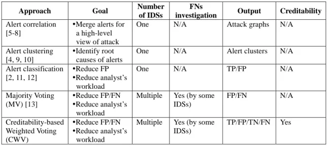
goals and methods of the above works, as summarized in Table 1, this work will focus
on the comparison of MV and CWV and evaluate the efficiency of two algorithms.
Table 1. Comparison of methods of alert post-processing.
Approach Goal Number
of IDSs
FNs
investigation Output Creditability
Alert correlation [5-8]
Merge alerts for a high-level view of attack
One N/A Attack graphs N/A
Alert clustering [4, 9, 10]
Identify root causes of alerts
One N/A Alert clusters N/A Alert classification
[2, 11, 12]
Reduce FP Reduce analyst’s workload
One N/A TP/FP N/A
Majority Voting (MV) [13]
Reduce FP/FN Reduce analyst’s workload
Multiple Yes (by some IDSs) FP/FN N/A Creditability-based Weighted Voting (CWV) Reduce FP/FN Reduce analyst’s workload
Multiple Yes (by some IDSs)
TP/FP/TN/FN Yes
2.2 Generation method of FP/FN datasets
In order to evaluate the detection capabilities of IDSs, the way to generate test
7
traces for evaluating FPs and FNs to measure the accuracy of the IDSs [13, 18].
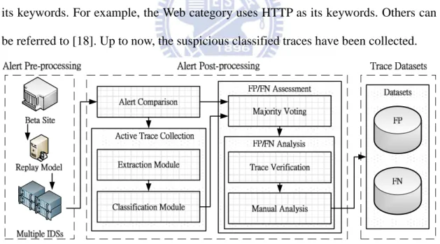
As shown in Figure 1, Lin et al. designed an Active Trace Collection (ATC) [18] to
actively extract and classify suspicious traces from real-world traffic captured in the
NCTU Beta Site [19]. First, in the extraction module, it uses a traffic replay tool to
replay the captured traffic to multiple IDSs. If an IDS detects specific behavior in the
traffic, it will trigger an alert. According to the IDSs’ alerts, the ATC finds out the
anchor packets that trigger the alerts by comparing five fields, i.e., source/destination IP
addresses, source/destination ports, and protocols, and then processes the packet and
connection association to extract each session into the packet traces. Second, in the
classification module, according to the alert messages, the ATC classifies the traces
into different categories by keywords. It defines ten categories, such as Web, File
Transfer, Remote Access, etc. Each category uses the corresponding protocol names as
its keywords. For example, the Web category uses HTTP as its keywords. Others can
be referred to [18]. Up to now, the suspicious classified traces have been collected.
Figure 1. Generation method of FP/FN datasets.
Besides, the detection of IDSs may be incorrect due to FPs and FNs. Lin et al. also
proposed a FP/FN Assessment (FPNA) [18], which analyzes the FP and FN cases and
investigates the causes of FPs and FNs. First, it finds out potential FPs and FNs of the
8
the corresponding extracted traces based on the alerts to the IDSs. This step verifies
whether the traces are reproducible to the original IDSs or not. Then, to confirm the
cases which are correct FPs or FNs, the reproducible traces are manually analyzed by
analysts. At the same time, the confirmed FP and FN cases and the causes of them are
recorded to generate the FP/FN datasets. This work further uses the traces and the
causes behind the FPs and FNs to investigate the creditabilities of IDSs.
In the following paragraphs, two case studies of the FP/FN analysis are taken as
examples to show why the benign traces are detected as malicious ones and the
malicious traces are not detected by IDSs. The investigation of FP/FN analysis is
illustrated with the description of activity, the corresponding signature, and the cause of
FP/FN, which are shown in the description, signature, and cause fields in Table 2 and
Table 3, respectively. In detail, first, the description of the malicious activity is referred
to Common Vulnerabilities and Exposures (CVE) [20]. Second, the corresponding
signature of the malicious activity is referred to Snort rule [1] as example if it exists.
Third, the cause of FP/FN is explained why the FP/FN occurs.
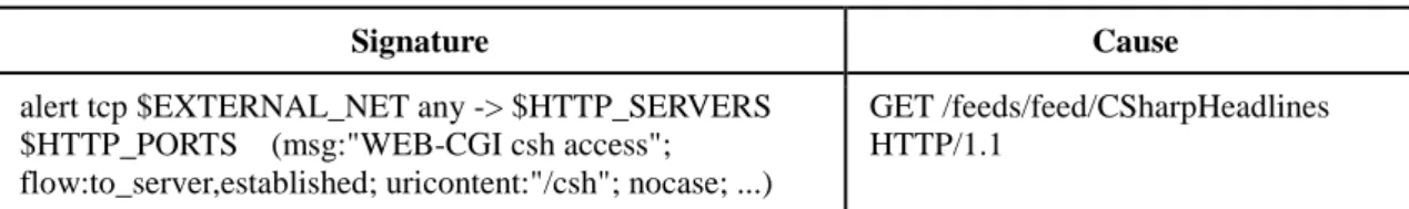
1) Table 2 illustrates a false positive case, “WEB-CGI csh access”, and the detail
analysis with Wireshark [21] of packet content is shown in Figure 2. The
execution of csh interpreter in the cgi-bin directory on a WWW site is detected by
just matching the “/csh” content in the request URI field. It often results in FP
because the signature design is too general and rough.
Table 2. A false positive in FP/FN analysis. Description
Perl, sh, csh, or other shell interpreters are installed in the cgi-bin directory on a WWW site, which allows remote attackers to execute arbitrary commands. (reference: CVE, 1999-0509)
Signature Cause
alert tcp $EXTERNAL_NET any -> $HTTP_SERVERS $HTTP_PORTS (msg:"WEB-CGI csh access"; flow:to_server,established; uricontent:"/csh"; nocase; ...)
GET /feeds/feed/CSharpHeadlines HTTP/1.1
10
Chapter 3 Problem Statement
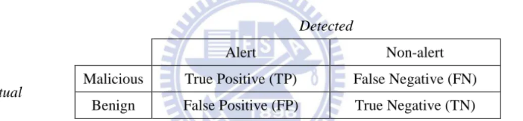
3.1 TerminologiesTable 4 defines a confusion matrix to represent the types of trace datasets with
IDSs’ detection. The rows represent the actual trace behavior such as malicious and
benign, and the columns represent the detection alarms such as alert or non-alert.
According to the corresponding relation between row and column elements, there are
four types of traces, True Positive (TP), False Positive (FP), True Negative (TN), and
False Negative (FN). TP and FP represent the IDS produces alert for malicious and
normal activities, respectively. Similarly, TN means the IDS does not produce alert for
a normal activity while FN does for a malicious activity.
Table 4. Confusion matrix definition. Detected
Alert Non-alert
Actual Malicious True Positive (TP) False Negative (FN)
Benign False Positive (FP) True Negative (TN)
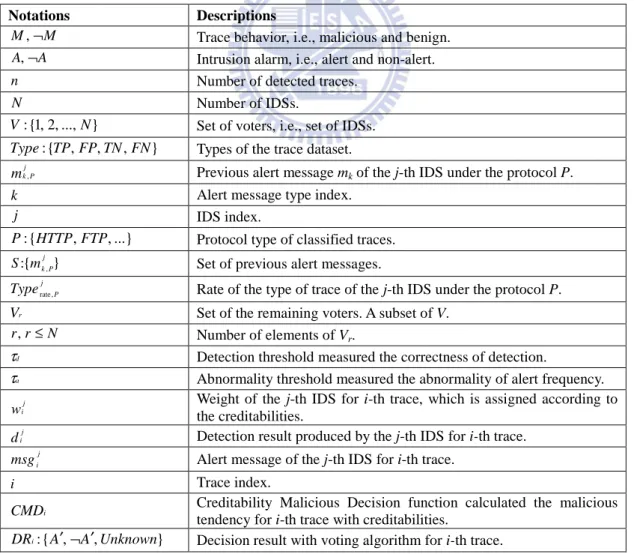
Table 5 defines the notations used in this algorithm. M and M¬ respectively denote malicious and benign. Based on the IDS detection, A and A¬ denote the presence or absence of an intrusion alarm, i.e., alert or non-alert, separately. Then, n
means the number of detected traces, i.e., how many traces marked with A there are. N
presents the number of IDSs involved in detection, and these N IDSs are a set V .
Moreover, whether all N IDSs having the voting rights depends on the voting
algorithm. According to the detection results, one of four types illustrated in Table 4
would occur, i.e., TP, FP, TN, or FN. Besides, suppose there are different k previous
alert messages of the j-th IDS under the protocol P , and mj P
k , records these
messages. Furthermore, a notation S is used to present a set of these messages. After the records, in order to investigate the creditabilities, we use probability to model
11
the rate of type of traces of the j-th IDS under each protocol by Typeratej ,P. However,
maybe not all IDSs are creditable enough, so two thresholds τd and τa are used to
choose parts of IDSs with suitable creditability. The set of the chose IDSs is a subset
of V and it is denoted as Vr. τd is the detection threshold whereas τa is the
abnormality threshold. Then, according to each IDS’s creditability, its corresponding
weight wj
i is assigned. d j
i and msg j
i are detection result and alert message of the
j-th IDS for i-th trace. Based on the above notations and definitions, CMDi can be
calculated for malicious tendency of i-th trace. Finally, based on the CMDi, DRi
represents a decision result for i-th trace, i.e., if the trace is malicious, benign, or
unknown.
Table 5. The notations used in Creditability-based Weighted Voting.
Notations Descriptions
M
M,¬ Trace behavior, i.e., malicious and benign.
A
A,¬ Intrusion alarm, i.e., alert and non-alert.
n Number of detected traces.
N Number of IDSs. } ..., , 2 , 1 { : N
V Set of voters, i.e., set of IDSs. } , , , { : TP FP TN FN
Type Types of the trace dataset.
mk ,jP Previous alert message mk of the j-th IDS under the protocol P.
k Alert message type index.
j IDS index. ...} , , { : HTTP FTP
P Protocol type of classified traces. }
{ : m,
S kjP Set of previous alert messages.
Typeratej ,P Rate of the type of trace of the j-th IDS under the protocol P.
r
V Set of the remaining voters. A subset of V.
N r
r, ≤ Number of elements of Vr.
d
τ Detection threshold measured the correctness of detection.
a
τ Abnormality threshold measured the abnormality of alert frequency.
wij
Weight of the j-th IDS for i-th trace, which is assigned according to the creditabilities.
dij Detection result produced by the j-th IDS for i-th trace.
msgij Alert message of the j-th IDS for i-th trace.
i Trace index.
i
CMD Creditability Malicious Decision function calculated the malicious
tendency for i-th trace with creditabilities. }
, , {
: A A Unknown
12
3.2 Problem description
In APP, on the one hand, the efficiency is low when alerts only come from one IDS,
as explained in Chapter 1. On the other hand, when alerts come from multiple IDSs, the
efficiency may also be low if APP disregards the different domain knowledge among
multiple IDSs. Moreover, due to the different domain knowledge, different IDSs may
have different detection results for a traffic trace. Hence, how to efficiently use these
results to make a good decision on the processed traffic trace is a problem.
The above description can be formulated as follows.
Given: (1) a training dataset T , (2) N IDSs, (3) sets of alerts produced by N
IDSs, (4) n corresponding processed traces.
Suppose: (1) the weight of j-th IDS is wj, (2) the alert produced by j-th IDS for i-th trace is aj
i .
Objectives: (1) model a series of weights { 1, 2, 3,..., }
w w w w N according to T , (2) design a function f (w ,aj) i j
i to make a decision on each trace.
To maximize the number of correct decisions, the number of FPs and FNs are
13
Chapter 4 Creditability-based Weighted Voting
This chapter details the Creditability-based Weighted Voting algorithm which
includes four components. The first component is the Creditability Modeling, which
investigates and models the IDSs’ creditabilities according to the past experience of
detection. Second, the Authority Selecting selects authorities of detection if they exist.
Third, the Voter Excluding excludes voters that cannot often perform well in detection.
Lastly, the Weighted Voting determines a trace where it belongs to.
4.1 Overview
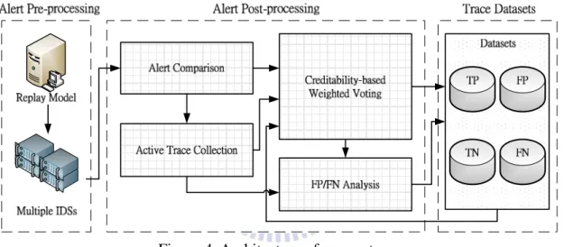
Figure 4. Architecture of our system.
The goal of this work is to increase the efficiency of alert post-processing when
alerts come from multiple IDSs, that is, to increase the accuracy of the corresponding
processed traces which actually belong to TP, FP, TN, or FN cases. Accordingly, the
generated TP/FP/TN/FN datasets can be not only used by IDS vendors to improve
their signature design, but also used to accumulate our knowledge of alerts.
For this goal, as shown in Figure 4, the Active Trace Collection collects and
classifies the suspicious traffic traces which are replayed to multiple IDSs by
comparing the alerts produced by IDSs. Since the detection of IDSs could be incorrect,
i.e., FP and FN, the FP/FN Analysis investigates the causes of FPs/FNs using the
14
ground truth. Based on the Datasets and the accumulated knowledge of alerts, this
work therefore proposes a Creditability-based Weighted Voting to make a decision on
the suspicious traffic trace more accurately.
Creditability-based Weighted Voting
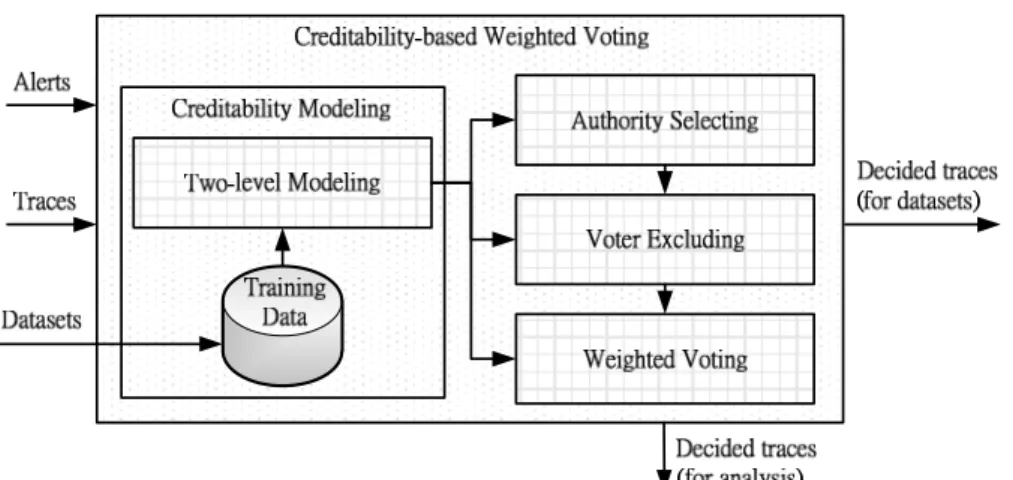
Figure 5. Architecture of Creditability-based Weighted Voting.
The key idea of the Creditability-based Weighted Voting to increase the
efficiency of alert post-processing is investigating the IDSs’ creditabilities and
deciding the traces more accurately with the corresponding creditabilities.
Hence, the Creditability-based Weighted Voting is constructed with some
components. As shown in Figure 5, from the Datasets, the Creditability Modeling
selects the significant types of traces to set up the Training Data and uses the
Two-level Modeling to model the IDSs‘ corresponding creditabilities for different
types of traces. Since each IDS could not perform well on all types of traces, we
consider that some IDS performs well or not on some type of trace or some alert.
Therefore, investigating the creditabilities only for all types of traces is not enough.
However, based on the creditabilities, first, the Authority Selecting selects the IDS
with high detection capability to be an authority if it exists. Secondly, the Voter
Excluding excludes the voter that cannot usually detect the malicious traffic in
detection. Third, the Weighted Voting decides the trace where it tends to, i.e.,
15
4.2 CM: Creditability Modeling
Since each IDS could not perform well on each alert or each type of trace, the
CM is designed to investigate and model the detection capabilities of IDSs for
different types of traffic with two levels. The two-level is especially designed in terms
of the categorization of signature definition. An alert message, the description of a
suspicious activity in a signature, comprises both or either two factors, i.e., protocols
and malicious types. Hence, investigating the alert can consider both two factors.
Besides, based on the protocol, which is the most common categorization, the
detection capability on protocol factor can also be investigated. Thus, it is reasonable
to make use of two levels to model the creditability. As shown in Figure 5, the CM
includes two components. One is Training Data and the other is Two-level Modeling.
TD: Training Data
According to the TP/FP/TN/FN traces confirmed from the FP/FN analysis, the
CM selects the significant types of traces to set up the TD. The selection policies are
based on the proportion of appearances in traffic and the number of corresponding
defined signatures. If both of them are high, the CM will identify the types of traces as
significant ones and select them into TD.
TLM: Two-level Modeling
Based on the TD, the TLM counts two detection capabilities for an IDS. One is
for Alert Message level (AML) and the other is for Protocol level (PL). Just as the
name implies, each AML’s detection capability depends on the correctness of an alert
message and the detection capability of PL is based on some protocol. Therefore, the
conditional probability of each element of the confusion matrix can be calculated as
follows.
16
analysis can be calculated as P(M |m , )
j P k
j with conditional probability,
) 1 ( , ] , 1 [ , ) ( ) ( ) | ( , , , j N m t m c m M P j P k j P k j P k j = ∈ where t(m , ) j P k and c(m , ) j P
k are the total number and the correct number of m j
P k , .
Second, in PL, we define the successful detection rate and successful ignorance
rate as Pj(M |A) and Pj(¬M |¬A) to mean the correct detected malicious traces
and ignored benign ones, respectively. Based on (1), the successful detection rate is
calculated as ) 2 ( , ] , 1 [ , ) ( ) ( ) ,..., , | ( ) | ( 1 , 1 , , , 2 , 1 j N m t m c m m m M P A M P h k j P k h k j P k j P h j P j P j j ∈ ∑ ∑ = = = =
where h is the number of all alert message types of j-th IDS under the protocol P.
Besides, according to the Bayes’ theorem and Typerate,j P, the successful ignorance rate is calculated as ) 3 ( . ] , 1 [ , ) ( ) ( ) ( ) | ( rate, rate, rate, N j FN M P TN M P TN M P A M P j P j P j P j ∈ ⋅ + ⋅ ¬ ⋅ ¬ = ¬ ¬
As a result, for each IDS, it has a creditability table which comprises three vectors, i.e.,
) | (M m , P j P k j , Pj(M |A) and Pj(¬M |¬A).
4.3 AS: Authority Selecting
Selecting authorities with relatively low FP and FN
Based on the investigation of detection capabilities of IDSs for different types of
traces, the AS finds that sometimes some IDSs have much higher creditabilities than
others. In other words, the lower FP and FN rates could result in higher creditabilities.
Thus, comparing with other IDSs, if the creditabilities of some IDSs are high enough
17
detection and selects these IDSs to be authorities.
The procedure of the AS includes three steps. First, for each type of trace, the AS
sorts the FP and FN rates of every IDS from high to low respectively. Then, the AS
separately calculates the average values L1 and L2 of FP and FN rates of the IDSs
listed after three-quarters of all IDSs since the concept of mean in Statistics. Third, the
IDSs will be selected to be the authorities of detection by the AS when their FP and
FN rates are both lower than L1 and L2.
Deciding traces by authorities if they exist
Finally, there are three cases: no authority, one authority, or multiple authorities.
If no authority occurs, the CWV will enter the Voter Excluding and then Weighted
Voting. When there is one authority, the traces will be decided directly by that
authority. Otherwise, the CWV will enter the Weighted Voting and the traces will be
decided by the multiple authorities.
4.4 VE: Voter Excluding
The VE is designed to exclude the voters which cannot usually perform well in
detection. Based on the concept, the VE excludes the voters according to two views.
One is the TP/FP rates and the other is alert frequency.
Excluding voters with low TP and high FP
First, according to the TP and FP rates, the VE excludes the voters which have
TP is less than detection threshold τd while FP is more than τd. The reason is that
some IDSs produce more incorrect detection than correct detection. The VE then
assumes that the IDSs are not strong enough and excludes them.
Excluding voters with abnormal alert frequency
Second, based on the alert frequency, the VE assumes that the IDSs having the
abnormal alert frequency are unusual. The reason is that some IDSs always produce
18
same type of trace, some IDS does not produce any alert while others do. Moreover,
the IDS, which has the detection function in the type of trace, does not produce any
alert that means its corresponding signature design is doubted. Thus, when every IDS
processes the same type of trace, if either the alert rate or the non-alert rate is more
than τa, the IDSs will be excluded by the VE.
4.5 WV: Weighted Voting
Calculating the malicious tendency
After the VE excludes some voters, or there are multiple authorities, the WV is
processed with proper voters. The WV assigns the weights to the corresponding voters
according to the creditabilities. Then, when processing the traces one by one, the WV
designs a Creditability Malicious Decision Function, CMD to calculate the degree of
tendency towards malicious activity. For i-th trace, its CMDi is calculated as
) 4 ( , ] , 1 [ , , ) ( , ) | ( 1 ) ( ) ( , ) | ( ) ( ) ( , ) | ( , , j V i n A d if A M P S msg A d if A M P S msg A d if msg M P T r j i j j i j i j j i j i j i j i j i ∈ ∈ ¬ = ¬ ¬ − ∉ ∧ = ∈ ∧ = = ) 5 ( . ] , 1 [ , 1 ) ( , T, i n r T CMD r V j j i j i i = ∑ ∈ ∈
In (5), the CMDi has three conditions to calculate Ti, j respectively. The first condition
is the j-th IDS produces an alert and the corresponding alert message belongs to the
previous alert message set. It can be detailed to AML with Pi,j(M |msgij). Secondly, the j-th IDS produces an alert but the alert message does not belong to the previous
alert message set. It can only be calculated in PL with Pj(M |A). Third, the j-th IDS does not produce an alert. It is calculated in PL with Pj(¬M |¬A).
Making a decision with malicious tendency
Finally, the WV makes a decision on i-th trace with DRi to decide the trace is
19
the DRi is benign if the CMDi is less than β. Hence, the DRi is formulated as
) 6 ( , , 1 , 0 ], , 1 [ , , ) ( , ) ( , , , α β β α β α ≤ < < ∈ < ′ ¬ > ′ = i n otherwise Unknown T CMD if A T CMD if A DR i i j j i i i
where A’ means the i-th trace is decided as malicious trace while ¬A’ means the i-th
trace is decided as benign one.
4.6 Example of Creditability-based Weighted Voting
Assume there are seven IDSs (i.e., N = 7), which detect the same traffic and
produce the corresponding alerts. By comparing the alerts, the HTTP traces can be
collected and are taken as examples here. After the FP/FN analysis, the TP/FP/TN/FN
datasets can be set up. Next, the CM set up the TD according to the datasets and then
uses the TLM to model the seven IDSs’ corresponding creditabilities respectively. It
first calculates TPj HTTP rate, , FP j HTTP rate, , TN j HTTP rate, , and FN j HTTP
rate, . Then, in AML,
the S is set up with the correct rates of the previous alert messages which are
calculated as P(M |m , )
j HTTP k
j . Next, in PL, it calculates the successful detection rate
) | (M A
Pj and successful ignorance rate Pj(¬M |¬A), which are shown in Table 6.
After the CM, the other three components of the procedure of the CWV can
process with the two-level creditabilities. First, in AS, the L1 and L2 are 0 and 0.51
separately. By comparing every IDS’s FPj HTTP
rate, and FN
j HTTP
rate, with L1 and L2
respectively, there is no authority in detection. Second, in the VE, the 3-rd IDS is
excluded according to the TP/FP rates. The 1-th, 4-th, 5-th and 6-th IDSs are excluded
according to the abnormal alert frequency. Hence, after the VE, the remaining voters
are the 2-nd and the 7-th IDSs. Finally, in the WV, when processing the 87-th trace,
the 2-nd IDS produces an alert and the alert message is “IBM Lotus Domino
20
not produce any alert. Besides, the creditability of the 2-nd IDS of the alert message
in AML, P87,2(M |msg872) is 0.83. The creditability of the 7-th IDS of the non-alert
in PL, P7(¬M |¬A) is 0.80. Therefore, the CMD87 is calculated as (0.83+(1-0.80))/2, that is, the result of the CMD87 is 0.52. Because the value is larger
than 0.5 (α = 0.5), the DR87 is A’ which means the 87-th trace is decided as malicious
one.
Table 6. Two-level creditabilities results of example run.
Creditabilities IDS1 IDS2 IDS3 IDS4 IDS5 IDS6 IDS7
) | (M A Pj - 0.46 0.03 - 1.00 - 0.51 ) | ( M A Pj ¬ ¬ 0.71 0.78 0.52 0.71 0.75 0.71 0.80 ) | ( 87 , 87 M msg
21
Chapter 5 Evaluation and Observation
In this chapter, the detection capabilities of multiple IDSs and the performance of
the CWV are evaluated. First, the IDSs’ corresponding creditabilities of different
types of traffic traces modeled by the CM are illustrated. Second, the Accuracy, TPR,
TNR and Efficiency are used to evaluate the voting algorithms.
5.1 Trace selection and experiment environment Trace selection
As mentioned in Chapter 4.2, the selection policies are based on the rates of
appearances in traffic and the rates of number of corresponding signatures. If both of
them of some type of trace are significant, this type of trace will be selected. First,
according to the ten categories classified by ATC [18], we investigate the traffic in
Beta Site [19] during the period from September 1, 2010 to February 1, 2011 to
understand the frequent appearance categories in traffic. Second, we take the rule
version 2.9 of Snort as example to investigate the signature classification and
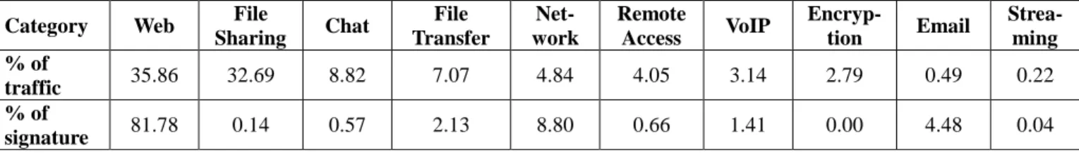
distribution. The investigation result of the above policies is shown in Table 7. It
obviously represents that Web, File Transfer, and Network are significant types.
Moreover, Remote Access is more familiar than VoIP to us in our experience. In
addition, the signatures in Chat are usually chat programs detection which used to be
against corporate policy in normal traffic [1]. Furthermore, in Web, File Transfer,
Network and Remote Access, we select the most popular protocol, respectively.
Hence, we decide the four types of traces, i.e., HTTP, FTP, NetBIOS and TELNET.
Table 7. Investigation result of trace selection.
Category Web File
Sharing Chat File Transfer Net- work Remote Access VoIP Encryp-tion Email Strea-ming % of traffic 35.86 32.69 8.82 7.07 4.84 4.05 3.14 2.79 0.49 0.22 % of signature 81.78 0.14 0.57 2.13 8.80 0.66 1.41 0.00 4.48 0.04 Experiment environment
22
The real-world traffic is captured from the NCTU Beta Site [19], during the
period from September 1, 2010 to February 1, 2011. It then uses a traffic replay tool
(e.g., tcpreplay) to replay captured raw traffic to multiple IDSs. Seven IDSs are
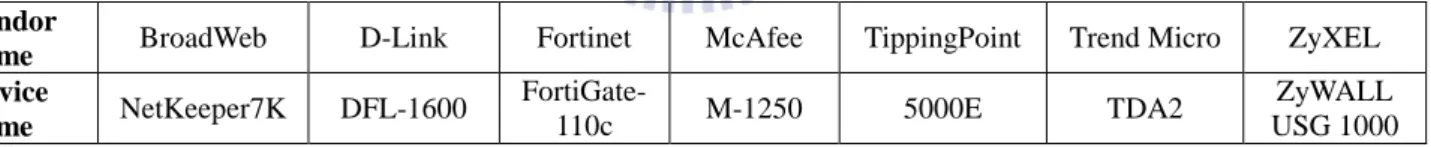
involved in the classification, which are shown in Table 8. Table 9 presents the
number of four selected types of traces. The ratio of malicious traces to benign ones is
about 4 to 6. The benign traces rate is not so expected high since we expect to avoid a
flood of the benign traces dominating the results in this experiment. During the period,
the two dominant types of trace are HTTP and NetBIOS. In the HTTP traffic, 39% of
the traces are malicious, meaning HTTP applications are frequently exploited. In the
NetBIOS traffic, 62% of the traces are malicious, meaning the vulnerabilities of
NetBIOS are usually targeted by attacker. Here, we choose the traces collected in the
first two months to be the training data while the traces of the latter three months to be
the processing data. The former is as input for the CM to set up the TD, and the latter
is as input for the CWV one by one.
Table 8. Seven IDSs Information. Vendor
name BroadWeb D-Link Fortinet McAfee TippingPoint Trend Micro ZyXEL
Device name NetKeeper7K DFL-1600 FortiGate-110c M-1250 5000E TDA2 ZyWALL USG 1000
The parameters in the CWV are set as follows. In the VE, the detection threshold
d
τ is set 0.5 while the abnormality threshold τa is set 0.9. In the WV, the values of α
and β are both set 0.5. Moreover, we discuss these parameters in Chapter 5.3.
Table 9. Statistics of number of traffic traces.
(a) Training data (b) Processing data
Type Malicious Benign Total Type Malicious Benign Total
HTTP 46 72 118 HTTP 57 86 143
FTP 22 74 96 FTP 29 77 106
NetBIOS 66 47 113 NetBIOS 87 46 133
TELNET 4 31 35 TELNET 5 42 47
23
5.2 Experiment results of investigation of creditabilities
In the CM evaluation, this work takes seven IDSs, which are called IDS1,
IDS2, …, and IDS7, respectively, as examples to represent the IDSs’ corresponding
creditabilities of different types of traffic traces in two levels.
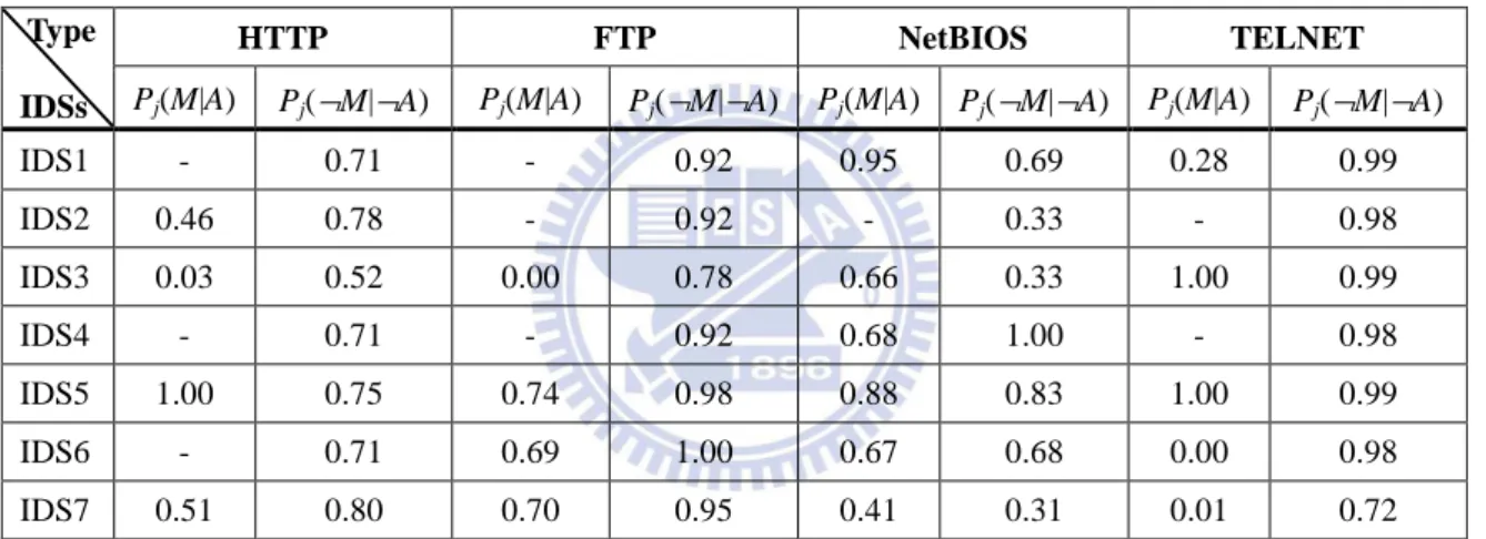
Protocol level
As mentioned in Chapter 4.2, the successful detection rate and successful
ignorance rate are defined as Pj(M |A) and Pj(¬M |¬A) , respectively, to
represent the detection capabilities for PL. As shown in Table 10 (a), first, the value of
detection rate is ‘-‘ that means uncalculated, that is, the IDS does not produce any
alert for the type of traces. Secondly, some values of detection rate are 0.00 since the
alerts result from common commands used, i.e., the traffic are always benign. For
example, some alerts produced by the IDS5 for FTP traces result from FTP common
command used. Third, some values of detection or ignorance rates are 1.00. The
observed reason is the definition of signature for the type of traces is more precise.
For instance, the type of alerts produced by the IDS5 for TELNET traces is only one
and is correct in our investigation. Besides, the IDSs’ detection capabilities for
different protocols are different. In our investigation, for HTTP, the IDS2, IDS5 and
IDS7 have higher creditabilities. Then, for FTP, the IDS5, IDS6 and IDS7 have higher
creditabilities. Next, for NetBIOS, the IDS1, IDS4, IDS5 and IDS6 have higher
creditabilities. Finally, for TELNET, the IDS3 and IDS5 have higher creditabilities.
Generally, the IDS5 achieves appreciable successful rates under each protocol.
Alert Message level
As mentioned in Chapter 4.2, the correctness of a previous alert message is
defined as P(M |m , )
j P k
j to represent the detection capability for AML. Table 10 (b)
24
creditabilities, in our investigation. Besides, some of them result from the same traffic
with same suspicious activity, and therefore, these are grouped into one to represent.
1) The first two “URL.DirectoryTraversal.Suspicious” and “HTTP: Attempt to
Read Password File” alerts result from the same traffic with the request URI
string “../../../../../../../etc/passwd”. The former alert results from the string “../../”.
The latter alert results from the string “/etc/passwd”. These malicious activities
could obtain the private information or access the files on the file system.
2) The “FTP: MKDIR Command Used” alert results from the FTP MKD command
used. The observed malicious activity is the MKD and CWD commands are used
alternately, which means the intruder creates a directory, changes the working
directory to the created directory, and then creates the same directory alternately.
3) The “specifiers.BolinTech.DreamFTPServer.Format.String” alert results from the
malicious FTP request containing embedded format string specifiers, i.e., “user
%n”, “pass %n”, “retr %n” or “%n”.
4) The “SOLARIS.TELNETD.AUTHENTICATION.EXP”, “Telnet: Login Bypass
(General)”, and “Solaris Telnetd Authentication Bypass Vulnerability” alerts
result from the argument injection via USER environment variable. The Solaris
telnet daemon misinterprets "-f" sequences as valid requests to skip the
authentication. However, the alert may be FP when the target is a non-Solaris
telnet server.
5) The
“NetPathCanonicalize.SRVSVC.MicrosoftWindows.MS08-067.Buffer.Overflow”
alert results from the RPC API NetPathCanonicalize() function exploited with a
crafted path. The successful overflow exploit could allow a remote attacker to
execute arbitrary code or crash the service. However, the alert may be FP when
25
6) The “IBM Lotus Domino Accept-Language Buffer Overflow” alert results from
the long length of Accept-Language field, e.g., 100. The observed malicious
activity is the duplicated language code appears frequently, while the alert may
be FP when the abnormal language code does not exist.
7) The “WEB-MISC robots.txt access” alert results from the file robots.txt accessed
directly. The malicious activity could gather the information about the target site.
However, the alert may be FP when some search engine’s robot checks robots.txt
for information about the site.
Table 10. Experiment results of investigation of creditabilities. (a) Protocol level – successful detection and ignorance rates for each IDS. Type
IDSs
HTTP FTP NetBIOS TELNET
Pj(M|A) Pj(¬M|¬A) Pj(M|A) Pj(¬M|¬A) Pj(M|A) Pj(¬M|¬A) Pj(M|A) Pj(¬M|¬A)
IDS1 - 0.71 - 0.92 0.95 0.69 0.28 0.99 IDS2 0.46 0.78 - 0.92 - 0.33 - 0.98 IDS3 0.03 0.52 0.00 0.78 0.66 0.33 1.00 0.99 IDS4 - 0.71 - 0.92 0.68 1.00 - 0.98 IDS5 1.00 0.75 0.74 0.98 0.88 0.83 1.00 0.99 IDS6 - 0.71 0.69 1.00 0.67 0.68 0.00 0.98 IDS7 0.51 0.80 0.70 0.95 0.41 0.31 0.01 0.72
(b) Alert Message level – top ten accurate alert messages.
Rank Alert messages P(M|m , )
j P k j
1 URL.DirectoryTraversal.Suspicious 1.00 1 HTTP: Attempt to Read Password File 1.00
1 FTP: MKDIR Command Used 1.00
1 specifiers.BolinTech.DreamFTPServer.Format.String 1.00 1 SOLARIS.TELNETD.AUTHENTICATION.EXP 1.00
1 Telnet: Login Bypass (General) 1.00
7 NetPathCanonicalize.SRVSVC.MicrosoftWindows.MS08-067.Buffer.Overflow 0.89 8 IBM Lotus Domino Accept-Language Buffer Overflow 0.83 9 Solaris Telnetd Authentication Bypass Vulnerability 0.80
10 WEB-MISC robots.txt access 0.75
26
Evaluation metrics
Let TPtraces be the number of malicious traces which are correctly determined,
FNtraces be the number of malicious traces which are not determined, TNtraces be the
number of benign traces which are correctly classified, FPtraces be the number of
benign traces which are incorrectly determined as malicious ones.
This work uses the Accuracy, TPR, and TNR metrics [22] for the voting
algorithm in the evaluation. The Accuracy is evaluated with the percentage of whole
traces that are determined precisely. This is a commonly used metric for overall view
of evaluation. . % 100 × + + + + = traces traces traces traces traces traces FN TN FP TP TN TP Accuracy
In detail, the TPR is evaluated with the percentage of malicious traces that are
correctly caught as malicious ones, while the TNR is evaluated with the percentage of
benign traces that are correctly passed as benign ones.
. % 100 , % 100 × + = × + = traces traces traces traces traces traces FP TN TN TNR FN TP TP TPR
There is a tradeoff between TPR and TNR. It is required to evaluate the
performance of voting algorithm on both TPR and TNR. Like the F1 score [23] which
is a measure of a test's accuracy, this work defines a similar measure for the efficiency
of voting algorithm. The Efficiency takes the harmonic mean of TPR and TNR, given
by: . % 100 1 1 2 × + = TNR TPR Efficiency
Higher value of Efficiency indicates that the voting algorithm performs better on not
only TPR, but also TNR.
Experimental evaluation results
30
accuracy can be 100% when the values of α and β are 0.7 and 0.1, respectively.
However, the range between α and β is large, 0.6 (= 0.7 – 0.1), so the number of
unknown cases is up to 55% of that of total processed traffic traces. Hence, α and β
can be tuned according to the tradeoff between the accuracy of decided traces and the
number of unknown traces that need to be analyzed manually.
5.4 Differences between CWV and each IDS in percentages at FP and FN
Table 11 shows the percentages of FP and FN of CWV and each IDS for
different types of traces. Some IDSs have FP and FN values with 0% and 100% since
these IDSs do not produce alert for this type of traces. This also means these IDSs
miss the signatures. Secondly, the FP of IDS3 is 100% because the alerts result from
common command used, such as “FTP GET command”. Third, the FP and FN of
IDS5 are 0%. The observed reason is the type of alerts produced by IDS5 is only one,
and the message is “SOLARIS.TELNETD.AUTHENTICATION.EXP” that is a
precise signature in our investigation, i.e., the creditability of the message is 1.0.
Actually, the corresponding traces are always malicious ones in analysis. Besides, for
NetBIOS traces, most IDSs produce many alerts that result in more FPs for each IDS,
while for other types of traces, some IDSs produce alerts that result in more FNs.
Table 11. Percentages of FP and FN of CWV and each IDS.
HTTP FTP NetBIOS TELNET FP FN FP FN FP FN FP FN IDS1 0 100 0 100 63.04 5.17 0 100 IDS2 26.74 94.74 0 100 0 100 0 100 IDS3 63.95 100 100 86.21 80.43 1.15 2.38 40.00 IDS4 0 100 0 100 25.53 7.58 0 100 IDS5 0 98.25 0 48.28 52.17 9.20 0 0 IDS6 0 100 0 13.79 67.39 1.15 0 100 IDS7 9.30 5.26 0 48.28 39.13 82.76 97.62 80.00 CWV 2.33 7.02 0 13.79 4.35 9.20 0 0
31
and FN are shown in Table 12. First, some IDSs detect better than the CWV partially
because the value of FP or FN in percentage is negative, but no IDS can individually
detect well in both FP and FN. Second, the CWV performs well in most cases for all
types of traces by leveraging different detection capabilities among IDSs which are
shown in different values of FP and FN. It is demonstrated that the average
percentages of FP and FN reduction between CWV and each IDS are 21% and 58%.
Table 12. Differences between CWV and each IDS in percentages at FP and FN.
HTTP FTP NetBIOS TELNET FP FN FP FN FP FN FP FN IDS1 -2.33 92.98 0 86.21 58.69 -4.08 0 100 IDS2 24.41 87.82 0 86.21 -4.35 90.8 0 100 IDS3 61.62 92.98 100 72.42 76.08 -8.05 2.38 40.00 IDS4 -2.33 92.98 0 86.21 21.18 -1.62 0 100 IDS5 -2.33 91.23 0 34.49 47.82 0 0 0 IDS6 -2.33 92.98 0 0 63.04 -8.05 0 100 IDS7 6.97 -1.76 0 34.49 34.78 73.56 97.62 80.00 Average 11.95 78.44 14.29 57.15 42.46 20.37 14.29 74.29 5.5 Case studies
In this section, two case studies in the experiment are taken as examples to show
the TP case in CWV and FN in MV, and the TN case in CWV and FP in MV.
Case study I: TP case in CWV and FN in MV
In this case, the alert messages and the corresponding creditabilities are shown in
Table 13, while the trace content is illustrated in Figure 10. It is observed that the
attacker uses the command “USER –fadm” as the argument injection via USER
environment variable in environment option to attempt to bypass the authentication.
More information about Telnet environment option can be found in [24]. Furthermore,
the malicious content in hexadecimal is “ff fa 27 00 00 55 53 45 52 01 2d 66 61 64 6d”
obviously. However, this malicious trace can be correctly determined by the CWV
34
Chapter 6 Conclusions and Future Works
This work proposes the Creditability-based Weighted Voting (CWV) to reduce
both FPs and FNs and increase the efficiency of alert post-processing with multiple
IDSs. The CM leverages the domain knowledge among multiple IDSs by
investigating the detection capabilities of all IDSs and models the corresponding
creditabilities to them. From the experiment results of investigation of creditabilities,
we demonstrate the different IDSs’ detection capabilities by their creditabilities. In
detail, we observe that the signature design is the main factor on the correctness of
detection. Some IDS has more specific signature that results in fewer number of alerts
and FPs, while some IDS has more general signature that results in more number of
alerts and FPs. On the other hands, some IDS misses the signature, leading to FNs.
This work uses Accuracy, TPR, TNR, and defines Efficiency to evaluate two
voting algorithms, the CWV and the MV. The CWV can achieve the accuracy and the
efficiency up to 95% and 94%, which are much higher than the MV in comparison.
Besides, between the CWV and each IDS, the CWV performs well in most cases for
all types of traffic traces. It is demonstrated that the average percentages of FP and FN
reduction between the CWV and each IDS are 21% and 58%.
However, the CWV could make an incorrect decision in some situations. For
example, when processing the trace which triggers the new alert of some IDS, the
CWV only can use the corresponding creditability in PL of the IDS to determine the
trace. The incorrect result could then occur. Besides, if some IDS significantly
updates or modifies its signature database, which means the detection capability
changes greatly, the corresponding creditability would be almost useless. The WV
could make an incorrect decision on the trace. Hence, the frequency and the duration
35
future is the automation because it could increase the productivity and practicability
of this system. In foreground, the CWV keeps processing traffic traces one by one,
while in background, the creditability table for each IDS is updated with considering
36
References
[1] “Rule of Snort,” available at: http://www.snort.org/vrt.
[2] T. Pietraszek, “Alert classification to reduce false positives in intrusion detection,” July 2006.
[3] S. Axelsson, “The base-rate fallacy and the difficulty of intrusion detection,”
ACM Transactions on Information and System Security (TISSEC), vol. 3, no. 3,
pp. 186-205, 2000.
[4] K. Julisch, “Clustering Intrusion Detection Alarms to Support Root Cause
Analysis,” ACM Transactions on Information and System Security (TISSEC), vol. 6, no. 4, pp. 443–471, November 2003.
[5] P. Ning, Y. Cui, Douglas S. Reeves, “Constructing Attack Scenarios through Correlation of Intrusion Alerts,” Proc. 9th ACM Conference on Computer &
Communications Security (CCS 2002), pp. 245-254, Washington D.C.,
November 2002.
[6] P. Ning, D. Xu, C. Healey, R. St. Amant, “Building Attack Scenarios through Integration of Complementary Alert Correlation Methods,” Proc. 11th Annual
Network and Distributed System Security Symposium, February 2004.
[7] P. Ning and D. Xu, “Learning Attack Strategies from Intrusion Alert,” Proc.
ACM Conference on Computer and Communication Security (CCS ’03), October
2003.
[8] R. Sadoddin, and A. Ghorbani, “Alert correlation survey: framework and
techniques,” Proc. 2006 international Conference on Privacy, Security and Trust:
Bridge the Gap between PST Technologies and Business Services, vol. 380,
November 2006.
[9] K. Julisch, “Using root cause analysis to handle intrusion detection alarms,” Ph.D. dissertation, University of Dortmund, 2003.
[10] K. Julisch, “Mining Alarm Clusters to Improve Alarm Handling Efficiency,”
Proc. 17th Annual Computer Security Applications Conference (ACSAC), pp.
12–21, December 2001.
[11] T. Pietraszek, and A. Tanner, “Data mining and machine learning-Towards reducing false positives in intrusion detection,” Information Security Technical
Report, 10:169–183, 2005.
[12] T. Pietraszek, “Using Adaptive Alert Classification to Reduce False Positives in Intrusion Detection,” Lecture Notes In Computer Science, pp. 102-124, 2004. [13] I. W. Chen, P. C. Lin, C. C. Luo, T. H. Cheng, Y. D. Lin, Y. C. Lai and F. C. Lin,
“Extracting Attack Sessions from Real Traffic with Intrusion Prevention Systems,” Proc. IEEE Intl. Conference on Communications (ICC), June 2009.