估計基因網路及基因間函數結構之統計方法

國

立

交

通

大

學

統計學研究所

碩

士

論

文

估計基因網路及基因間函數結構之統計方法

Statistical Methods for Estimation of Genetic Networks

and Functional Structures between Genes

研 究 生：羅巧慧

指導教授：洪志眞 教授

洪慧念 教授

估計基因網路及基因間函數結構之統計方法

Statistical Methods for Estimation of Genetic Networks

and Functional Structures between Genes

研 究 生：羅巧慧 Student：Chau-Wui Lo

指導教授：洪志眞 博士 Advisors：Dr. Jyh-Jen Horng Shiau

洪慧念 博士 Dr. Hui-Nien Hung

國 立 交 通 大 學

統計學研究所

碩 士 論 文

A Thesis

Submitted to Institute of Statistics College of Science

National Chiao Tung University in Partial Fulfillment of the Requirements

for the Degree of Master

in Statistics June 2004

Hsinchu, Taiwan, Republic of China

估計基因網路及基因間函數結構之統計方法

研究生：羅巧慧 指導教授：洪志眞 教授

洪慧念 教授

國立交通大學統計學研究所

摘 要

我們提出一個利用統計方法來建構基因網路的方法。我們

將目標分成三個部分。第一部分是先探討兩個變數間是否

有關係存在？如果他們之間確實有關係，第二部分就是探

討他們是如何的相關？激發或是抑制?接著第三步即是去

找出他們相關的方向。在資料分析的部分，利用了蒙地卡

羅模擬分析來展示我們所提出方法的分析效率，並且最後

我們也把提出的方法應用在酵母菌資料上來作個討論。

Statistical Methods for Estimation of Genetic Networks

and Functional Structures between Genes

Student：Chau-Wui

Lo

Advisors：Dr. Jyh-Jen Horng Shiau

Dr. Hui-Nien Hung

Institute of Statistics

National Chiao Tung University

Abstract

We propose a procedure for constructing gene networks using statistical methods. Three issues are considered. First, is there a relationship between a pair of genes? Second, how do they relate, repress or activate? Third, what is the related direction? By considering the relationship of a pair of genes at a time, our method gives not only the relation (activate, repress) but also the direction for each pair of genes. We conduct Monte Carlo simulations to show the effectiveness of the proposed method. Finally, the method is applied to the Sacharomyces cerevisiae gene expression data as an illustrative example.

誌 謝

在交大這兩年，讓我受益良多，不但學習到專業知識，遇到

很多的朋友，更學習到如何解決問題及主動學習的精神。感謝指

導教授洪志真老師及洪慧念老師熱心的指導與照顧，也很感謝同

學們寶文、崢珮、超毅、欣妤、怡均、淑真、忠庭、政輝、志浩、

慶富、文祥、翠英、淑靜、坤民、宏元、宇青的包容和陪伴及博

士班學長達叔、宏嘉、牛哥、泰賓的照顧。除此之外很感謝我的

家人的支持與鼓勵。能夠順利完成碩士學位，非常感謝各位的支

持。

羅 巧 慧 謹誌于

國立交通大學統計學研究所

中華民國九十三年六月

Contents

Chinese Abstract ---i

English Abstract ---ii

Acknowledgment ---iii

Contents ---iv

1. Introduction ---1

2. Literature Reviews ---3

2.1. Casual Effect ---3

2.2. Bayesian Network ---5

2.3. Using Bayesian Network and Nonparametric Regression to Analyze

the Causal Effect between Variables ---6

2.4. Using Nonparametric Regression Method to Analyze the Casual

Effect between Variables ---8

2.5. Using Smooth Response Surface Methodology to Construct Gene

Networks---11

3. Methodology ---15

3.1. Motivation ---15

3.2. Proposed Methods ---15

4. Empirical Studies ---23

4.1. Monte Carlo simulation ---23

4.2. A study on Causal Relationships ---28

4.3. Real data Analysis ---29

5. Discussions ---33

References ---35

Tables ---38

1. Introduction

In the recent years, a large amount of gene expression data has been collected and estimating a gene network has become one of the popular topics in the field of bioinformatics. The knowledge of the coding sequences of virtually every gene in an organism has enabled the development of technology to simultaneously monitor the expression of all the genes. Due to the curse of dimensionality and complexity of the expression data, it is not an easy task to find structures, which are buried in noise. Several methodologies have been proposed for constructing gene network based on gene expression data, such as Boolean networks [1,2,3,4,18,20], differential equations [6,9], Bayesian networks [10,11,14,15,16,25,26], nonparametric regression [7,8] and a smooth response surface methodology [27]. Some of them will be introduced in reviews. To extract the effective information from micro array gene expression data, theory and methodology are expected to be developed.

We use a simple example to introduce the causal and effect relationship. The height may cause the weight, but the weight cannot influence the height. We can see that there are inspire (active) or depress (repress) between those two variables like the relations between genes. The causal and effect relationship has been discussed in many fields, such as medicine, industry and society. For example, doctors reason the causes of diseases by their accumulated experiences, industrial engineering realize the actual breakdown causes using experimental designs. In this study we are interested in finding a good method to discover the direction and relation between the genes that actually have cause-effect relationship.

We propose a method to find the relationships between genes using statistical methods. We consider the relation of a pair of genes at one time. If there are M genes,

then there are ₂M

C times need to be done. Our method gives not only the relations

(active, repress) but also the directions between genes. Our method can be divided into two parts by the distributions of the residuals. The second part of our proposed method is to discretize data first. Secondly find whether there is a relation between two variables or not. And also, find how they connected (active, repress). Third, find the directions. Details can be seen from the flowchart latter. The advantages of our method are we don’t need strong statistical assumption before using and compute rapidly. Especially when the sample size is small, the resulting graph size is still similar to the graph size of larger sample size. The shortcoming of our method is not sensitive to symmetric functional structures.

The rest of the paper is organized as follows. Section 2 gives a literature review on relate research works. Section 3 decides the proposed methodology. Section 4 presents the results of a simulation study and a real data analysis. Section 5 concludes the paper with a brief summary and discussion.

2. Literature Reviews

2.1 Causal Effect

In this section, we review these methodologies for finding the cause-effect relationships between variables. A simply causal and effect relationship can be decided as follows.

If X (cause/parent) causes Y (effect/child), then manipulating the value of X affects the value of Y. On the other hand, if Y causes X, then manipulating the value of X will not affect Y. Let ,x i_i =1,...,n be the variables under study. A functional causal model

in general form consists of a set of equations of the form

(x_i = f pa u_{i i}, ),_i i=1,....,n (2.1) where pa (connoting parents) stands for the set of variables judged to be immediate _i

causes ofX , _i represents the errors (or “disturbances”), and is the functional relationship between the variables. Equation (1) is a nonlinear, nonparametric generalization of the linear structural equation models (SEMs).

i U f( )⋅ , 1,..., i ik k i k i x α x u i n ≠ =

∑

+ = (2.2) In the linear model, corresponds to those variables on the right-hand- side of (2) that have nonzero coefficients.

i

pa

A set of equations in the form of (1) and in which each equation represents an autonomous mechanism is called structural model; if each mechanism determines the value of just one distinct variables (called the dependent variables), then the model is called a structural causal model or a causal model for short. To illustrate, Figure 1 depicts a canonical econometric model relating price and demand through the equations

1 1 ,

2 2 2,

p=b q+d w u+ (2.4)

where Q is the quantity of household demand for a product A, P is the unit price of the product A, I is the household income, W is the wage rate for producing product A, and represent error terms-unmodeled factors that affect the quantity and price, respectively (Goldberger, 1992). The graph associated with this model is cyclic, and the vertices associated with the variables are root nodes, conveying the assumption of mutual independence.

1

u

u₂

1, 2, , and

U U I W

The idea of autonomy (Aldrich, 1989), in this context, means that two equations represent two loosely coupled segments of the economy, consumers and producers. Equation (3) describes how consumers decide what quantity Q to buy and (4) describes how manufacturers decide what price P to charge. Like all feedback system, this too represents implicit dynamics; today’s prices are determined on the basis of yesterday’s demand, and these prices will determine the demand in the next period of transactions. The solution to such equations represents a long-term equilibrium under the assumption that the background quantities,

U

₁andU₂, remain constant. [19]

1 U I W U₂ Q P 1 d d2 2 b 1 b

Figure 1: Causal diagram illustrating the relationship between price (P), demand (Q), income (I), and wages (W).

2.2 Bayesian Network

A graph consists a set of vertices (or nodes) and a set of edges (or links) that

connect some pairs of vertices. The vertices of the graphs correspond to variables and the edges denote a certain relationship that holds in pair of variables. Two variables connected by an edge are celled adjacent. If every edge in a path is an arrow that points

from the first to the second vertex of the pair, we have a directed path. A graph with

directed path called is called a directed graph. Directed graphs may include directed

cycles (e.g., XÆY, YÆX), representing mutual causation or feedback process, but no

self-loops (e.g., XÆX). A graph that contains no directed cycles is called acyclic. A

graph that is both directed and acyclic is called a directed acyclic graph (DAG).

Undirected graphs, sometimes called Markov networks (Pearl, 1988b), are used

primarily to represent symmetrical spatial relationship (Isham, 1981; Cox and Wermuth, 1996; Lauritzen, 1996). Directed graphs, especially DAGs, have been used to represent causal or temporal relationships (Lauritzen, 1982; Wermuth and Lauritzen, 1983; Kirveri et al., 1984) and are known as Bayesian networks. Figure 2 is an example of a simple Bayesian network structure. This network structure implies several conditional independence statements:

( ; ), ( ;

| , ), ( ; , ,

| ), ( ; , ,

| ),

( ; , ).

I A E I B D A E I C A D E B I D B C E A and I E A D

(2.5)

The network structure also implies that the joint distribution has the product form

( , , , , ) ( ) ( | , ) ( | ) ( | ) ( ).

P A B C D E = P A P B A E P C B P D A P E (2.6)

E A

B D

C

A causal network can be interpreted as a Bayesian network when we are willing to make the Causal Markov Assumption: given the values of a variable’s immediate causes, it is independent of earlier causes.

2.3 Using Bayesian Network and Nonparametric Regression to Analyze the Causal Effect between Variables

A Bayesian network is a graph-based model of joint multivariate probability distributions that captures properties of conditional independence between variables. It consists two components. The first component, G, is a directed acyclic graph (DAG)

whose vertices correspond to the random variablesX₁,...,X . The second component,_n θ ,

describes a conditional distribution for each variable, given its parents in G. Together,

these two components specify a unique distribution on X₁,...,X . The graph G _n

represents conditional independence assumptions that allow the joint distribution to be decomposed, economizing on the number of parameters. The graph G encodes the

Markov Assumption: Each variableX is independent of its non-descendants, given its _i

parents in G.

By applying the chain rule of probabilities and properties of conditional independencies, any joint distribution that satisfies the Markov Assumption can be composed into the product form

1 1 ( ,..., ) ( | ( )), n G n i i P X X P X Pa X = =

∏

i (2.7) where PaG(X_i)is the set of the parents of X in G. The method of Bayesian network is _i

to select a proper graph G with the largest posterior probability after giving the prior probability. Imoto et al. (2002) proposed the criterion

1 ( ) 2 log ( | ) ( | ) G P i G G G i BNRC G π f x θ π θ λ θd = ⎧ ⎫ = − _{⎨ ⎬} ⎩

∫

∏

⎭ (2.8) whereπ_Gis the prior probability of the graph G, (π θ λ_G| )is the prior probability of

G

θ after giving parametric vectorλ , θ_G=(θ₁T,...,θ_nT)is the parametric vector in G,

j

θ is the parametric vector of model f , and _j

1 ( | ) ( | , ) P i G j ij ij j j f x θ f x p θ = =

∏

(2.9) 2 ( ) ( ) ( ) 1 1 2 2 2 ( ) 1 ( | , , ) exp 2 2 j ij q M j j j ij mk mk ik k m j ij ij j j j j x b p f x p γ γ σ σ πσ = = ⎡ _{⎛ ⎞} ⎤ ⎢ _⎜ − _⎟ ⎥ ⎢ _{⎝ ⎠} ⎥ = _⎢− _⎥ ⎢ ⎥ ⎢ ⎥ ⎣ ⎦

∑∑

(2.10)

wherex is the ith observation of jth variable, that is, if the number of observation is n _ij

then the observation of the jth variableX is j

x

1j

,...,

x

nj . We use to represent

the parents of

1j,...,

P Pnj

j

X .

p

ij is the vector with -dimension, i.e., the jth variable has

parents at the ith observation, and its kth component is . And use nonparametric

regression models for capturing the relationship between j q qj ( )k ij p ij x and in the form ( ) ( ) 1 ( ,..., ) j j j ij i iq p = p p ₁( ₁( )) ₂( ₂( )) .... ( ( )) , 1,..., ; 1,..., . j j j j j ij i i q iq ij x =m p +m p + +m p +ε i= n j= p (2.11)

where (m k_k =1,...,q_j)are smooth functions from R to R, and ε_ij(i=i,..., )n depend

independently and normally on mean 0 and varianceσj2. For mk, it is assumed that

( ) ( ) ( ) ( ) 1 ( ) ( ), 1,..., ; 1,..., . jk M j j j j k ik mk mk ik j m m p γ b p i n k q = =

∑

= = (2.12) where

{

₁ ( ),..., ( )

}

jk j k M k b b j j

is a prescribed set of basis functions (such as Fourior series, polynomial bases, regression spline bases, B-spline bases, wavelet bases and so on),

is the unknown coefficients and

( ) ( ) 1 ( ,..., ) jk j k M k

γ γ M is the number of basis. Bayesian jk

networks are to find G makes BNRC maximized.

models for capturing not only linear dependencies but also nonlinear structures between genes. Imoto et al. (2003) improved this method by using Bayesian networks and the nonparametric heteroscedastic regression, which is more resistant to the effect of outliers but it needs much time for determining the optimal graph. Tamada et al. (2003) proposed a motif detection method to estimate gene networks and combine microarray gene expression data and DNA sequences of regulatory regions of genes. It found that the motif information is useful for revising some incorrect relations in the network estimated by microarray alone. Imoto et al. (2003) proposed a method for estimating a gene network based on Bayesian networks from microarray gene expression data together with biological knowledge including protein-protein interactions, protein-DNA interactions, binding site information, existing literature and so on. Its proposed criterion can control the trade-off between microarray information and biological knowledge automatically. Kim et al. (2003) proposed a Bayesian network and nonparametric regression model for constructing a gene network from time series microarray gene data. This method can overcome a shortcoming of the Bayesian network model in the sense of the construction of cyclic regulations.

2.4 Using Nonparametric Regression Method to Analyze the Causal Effect between Variables

Different from linear regression analysis, nonparametric regression uses a roughness penalty that decreases as the fitting curve gets smoother.

Consider the n observations{(xi,yi),i=1,...,n}. Assume that the sample is ordered over the interval [a, b] with respect to the predictor values; that is,

b x x

a≤ 1≤...≤ n ≤ . To estimate the unknown smooth regression function by explicitly trading off fidelity to the data with smoothness of the estimate. For regression, the residual sum of squares is a natural measure of fidelity to the data, so the roughness

penalty estimator is the minimizer of =

∑

− +

∫

= b a n i i i g x g x dx y n g S 2 1 2 )) ( " ( )) ( ( 1 ) ( λ , (2.13) and the resulting cubic smoothing spline estimategˆbelongs to the Sobolev space

} . integrable square is g" , continuous absolutely are ' and | { ] , [ 2 g g g b a W₂ =

(2.14) Whereλ >0is the smoothing parameter. Ifλ=0, the smoothing spline becomes an interpolating spline that passes through each of the responsesy_i, while if

∞ →

λ ,gˆapproaches the linear least squares regression line. The smoothing spline is a linear estimator, so the vector of fitted valuesyˆ_i = gˆ(x_i) can be written as

. ) (

ˆ A y

y = λ The matrixA(λ)is called the hat matrix. λ can be chosen to minimize the

cross-validation score [17] , )] ( ˆ [ 1 ) ( 1 2 ) (

∑

= − = n i i i i g x y n CV λ

(2.15) where is the spline estimate based on all the observations except , evaluated at . It can be shown that for linear smoothers,

) ( ) ( i i x g x_i i

x

CV

(

λ

)

can be written as a function of

the fitted values (Green and Silverman, 1995) [17],

, ) ( 1 ) ( ˆ 1 ) ( 2 1

∑

= ⎥⎦ ⎤ ⎢ ⎣ ⎡ − − = n i ii i i A x g y n CV λ λ

(2.16)

whereAii(λ)is the ith diagonal element of the hat matrixA x( ). Aii(λ)is called the leverage value at since it measures the potential for the observed response to exert influence on the fitted value.

i

x y_i

A variation is generalized cross-validation (GCV) [17], which replaces each value1−A_ii(λ)with their average, . The generalized cross-validation

selector of , is the minimizer of

)] ( [ 1−n−1trace A λ GCV λ λ_, ˆ 2 1 2 1 )]} ( [ 1 { )] ( ˆ [ ) ( λ λ A trace n n x g y GCV n i i i − = − − =

∑

. (2.17)

Proposition 1. (Shiau, 1985) Letgˆ_λbe the smoothing spline estimator. Then

S(gˆ_λ)= yT(I−A(λ))y/n, (2.18) The following two propositions are given in Cheng (2003).

Proposition 2. ) , and is the mode of the posterior density after

giving the prior distribution. ( min arg

ˆ S g

gλ = g

Proposition 3. Assume that X and Y and E(X)=E(Y)=0, Var(X)=Var(Y)=1 , let , be n i.i.d. observations. Then

n i

y

xi, i), 1,...,

( = E(S(gˆ_λ))→1,asn→∞.

Cheng (2003) consider only the causal relationship between two variables X and Y.

If X is the parent (cause) and Y is the child (effect), then denote the cause-effect

relationship by XÆY. more specifically, the causal relationship between X and Y can be

described by the following causal models: Y =g X₁( )+ , where is a smoothing ε function and

1

g

ε is a random error with mean zero and independent of X. If X cannot be

simultaneously represented as ' 2( )

g Y + with Y independent of an random errorε ε'

,

then XÆY but not vice versa.

We shall call the method proposed in Cheng (2003) determing the causal direction between two random variables “SCORE” method. SCORE method simultaneously use nonparametric method to estimate and . Finally gets two score and

(Shiau, 1985), then use decision rules to determine the direction. 1 g g₂ S(gˆ₁) ) ˆ (g2 S

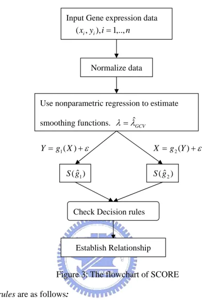
We simplify Chia Yu Cheng et al. (2003) as the following flow chart.

Input Gene expression data n i y xi, i), 1,.., ( = Normalize data

Use nonparametric regression to estimate smoothing functions. λ =λˆGCV

Figure 3: The flowchart of SCORE

Decision rules are as follows:

IfS(gˆ ) S(gˆ )then XÆY has a larger posterior probability than YÆX, i.e., X causes Y. 2

1 <

>

IfS(gˆ₁) S(gˆ₂)then YÆX has a larger posterior probability than XÆY, i.e., Y causes X.

IfS(gˆλ) is close to 1, then X ⊥Y (Cheng (2003) suggested , and Lu (2003) suggested ). 9 . 0 ) ˆ (g_λ > S ˆ ( ) 0.8 S g_λ >

We call the 0.9 or 0.8 “the threshold score of independence”.

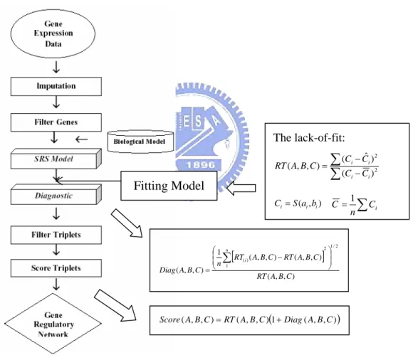
2.5 Using Smooth Response Surface Methodology to Construct Gene Networks

A smooth response surface algorithm proposed by Xu et al. (2002) is a sophisticated data mining technique for analyzing gene expression data and constructing gene networks. It uses a three-dimensional smooth response surface to capture the biological relationship between the target and activator-repressor. It also functionally

) ˆ (g₁ S S(gˆ₂) ε + =g₁(X) Y X =g₂(Y)+ε

Check Decision rules

describes triplets of activators, repressors, and targets, and their regulations in gene expression data. The diagnostic strategy in the algorithm is to evaluate the scores of the triplets so that those with low scores are kept and a regulatory network is constructed based on this information and existing biological knowledge. Xu et al. (2002) applied the method to two yeast gene expression data sets and reported that the predictions based on the identified triplets agree with some experimental data in the literature. This method provides a novel model with attractive mathematical and statistical features that make the algorithm valuable for mining expression or concentration information, help for determining the function of uncharacterized proteins, and can result in a better understanding of coherent pathways.

The smooth response surface method is decided as follows. First, transform the raw data over the time points into the interval [0, 1]. Let A be the activator and B be the repressor. The definition of the activator-repressor-target model is that a target gene C is controlled by both an activator gene A and a repressor gene B. Define a three-dimensional smooth response surface as S(A, B), which is a piecewise linear-quadratic polynomial on [0, 1] × [0, 1]. The triplets that follow the activator-repressor-target relationship should lie closely to the response surface.

The 3D response surface has the same purpose with a high dimensional decision matrix. The function S(A, B) maps two normalized values A and B onto a 3D surface, in order to describe a surface response value C .To ease decision-making, it uses some heuristic rules:

A high + B low Æ C high. A low + B high Æ C low.

As seen in Figure 3, a triplet (A, B, S(A, B)) represents the biological relationship that follows the pattern of a target S(A, B) controlled by an activator A and a repressor B as described in the activator-repressor-target model. The response surface captures the

biological model with features such as compactness, simplicity and visualization. The imputation and gene filtering steps are applied to remove noise from the data.

For each triplet (A, B, C), is the fitted value of a target C. The residual, , should be small, if the activator-repressor-target relationship is strong. The residual sum of squares measures the overall variation in C that is not explained in the response surface model. Then the lack-of-fit function RT(A, B, C), i.e., the ratio of the residual sum of squares and the total sum of squares, describes the proportion of variation in C that is not captured by the 3D response surface. A small value of lack-of-fit indicates that there is a strong activator-repressor-target relationship among A,

B, and C. The lack-of-fit formula is defined to filter the triplets in the initial screening.

To save storage and computation, only those triplets whose lack-of-fit values do not exceed a given constant RT are kept.

) , ( ˆ _{S A B} C= C Cˆ−

A diagnostic strategy Diag(A, B, C) is applied to check the reliability of the triplets after the initial filtering to measure robustness of the fitted model for each triplet (A, B,

C ). Xu et al. (2002) pointed out that the intensity measurement of gene expression at

one or two time points may deviate from the model and suggest that the measurement may be faulty and should be treated as an outlier. If such a value occurs at the i-th point,

then , i.e., the lack-of-fit of (A, B, C) when the i-th point (or the i-th

column) is left out, will differ greatly from RT(A, B, C). Diag(A, B, C) provides a summary measure over all time points for a given triplet. The diagnostic method is developed to refine the selected triplets and a score, which reflects the strength of the triplet interrelationship, is defined to rank the refined triplets. A larger Diag value would suggest that the information for the triplet is unreliable and should be removed for further consideration. Thus the criteria for selecting triplet candidates is: ) , , ( ) ( A B C RT_i Diag C B A Diag RT C B A

specified by users.

A final score is defined to measure the strength of the triplet interrelationship.

Score(A, B, C) is a function of the lack-of-fit value and the diagnostic measure, and

focuses primarily on the RT(A, B, C) value and secondly on the Diag(A, B, C) values. Triplets with low values of RT(A, B, C) and Diag(A, B, C) will have low scores, which indicate a close relationship among A, B, and C. Finally, a gene regulatory network is constructed based on the top scoring triplets. Figure 4 gives the flowchart of the smooth response surface algorithm.

The lack-of-fit:

∑

(Ci− )Ci

∑

− = ( ˆ)₂2 ) , , (ABC Ci Ci RT ) , ( i i i Sa b C = C=1

∑

C_i n Fitting Model [ ] ) , , ( ) , , ( 1 ) ( C B A RT n C B A Diag i ⎟ ⎠ ⎜ ⎝ = ) , , ( ) , , ( 1 2 / 1 2 C B A RT C B A RT n ⎟ ⎞ ⎜ ⎛ − ∑ (1 ( , , )) ) , , ( ) , , (ABC RT ABC Diag ABC Score = +

3. Methodology

3.1 Motivation

Xu et al. (2002) proposed the activator-repressor-target model to represent that each variable can find its activator and repressor and is controlled by the activator and repressor simultaneously. It is not clear whether there exists such a triplet relationship in reality. In this study, we consider pairs of genes instead of triplets.

Cheng (2003) proposed a score method to determine the relationship between two variables. But this method only determines the causal effect direction but no activate (+) / repress (-) information. Also, there is a problem of determining whether two variables are independent. Therefore, we use the method in next section to improve Cheng’s method.

3.2 Proposed Methods

We simplify our goal as finding the relation between two variables.

If X is the parent (cause) and Y is the child (effect), then we use XÆY to represent the causal effect relation between them. We assume X and Y have the regression relation: , where f is a smoothing function and is a random variable with mean zero and is independent of X. Sometimes, X can be represented as

with Y being independent of

Y=f (X)+ ε ε

'

g(Y)+ ε ε at the same time. This will hold when f is a ' linear function. When this happens, we denote the cause/effect reality byX↔Y.

2

R

Let and be the residuals of regressory Y on X and X on Y, respectively. The core idea of our method is that, if XÆY, then we should have the following result:

1

R

1 2 1 ˆ 2 ˆ

R ⊥X and R ⊥ Y, where R = −Y f (X) and R = −X g(Y). On the other hand, if YÆX, thenR₁ ⊥ X and R₂ ⊥ . Y

- + - +

-X⎯⎯+→Y, X⎯⎯→Y, X←⎯⎯Y, X←⎯⎯Y, X←⎯→Y, X←⎯→Y, X⊥Y. Arrow is the direction. The sign above the arrow represents activate (+) or repress (-).

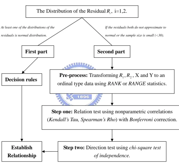
Our proposed method is divided into two parts by the patterns of the residuals , =1, 2.

i

R i

We summarize the method by the following flow chart.

The Distribution of the Residual R

We can use a graphical display, QQ plot, to check the normality of the residuals.

QQ plots are used to assess whether a data set has a particular distribution, or whether

two datasets have the same distribution. If two distributions are the same, then the plot will approximate a straight line. The extreme points have more variability than points toward the center. Or we can use Kolmogorov-Smirnov Goodness-of-Fit Test

Second part , i=1,2. i

At least one of the distributions of the residuals is normal distribution.

If the residuals both do not approximate to normal or the sample size is small (<30).

First part

Pre-process: TransformingR , X and Y to an ordinal type data using RANK or RANGE statistics.

2 1,R Decision rules

Step one: Relation test using nonparametric correlations (Kendall’s Tau, Spearman’s Rho) with Bonferroni correction.

Establish Relationship

Step two: Direction test using chi-square test

of independence.

(Chakravart, Laha, and Roy, 1967) [5] and Chi square Goodness-of-Fit Test (Snedecor and Cochran, 1989) [24] to compare the distribution of the residuals with normal. If the sample size is small, we suggest skip this part and go to second part.

First part: At least one of the distributions of the residuals is normal distribution. (We remark that this condition usually does not hold in our study.)

In this part we use the following Decision rule:

1. IfR is approximately normal and₁ R isn’t, then XÆY. ₂

2. IfR is approximately normal and₂ R isn’t, then YÆX. ₁

3. IfR and₁ R both are approximately normal, then₂ X ↔Y .

4. IfR and₁ R both are not approximately normal or the sample size is small, then ₂

go to second part.

From our experience, the chance of using the first part of our method is quite small.

Second part: When the residuals both are not approximately normal or the sample size is small (<30).

1 2

R and R

In this part, we divide the target into the following steps: Q1. Is there a relationship between those two variables? Q2. How do they relate? Repress (-) or activate (+)?

Q3. What is the related direction if they really have relationship?

Step one will solve the Q1 and Q2. Step two will give the answer to Q3.

If we want to know the relationship between two variables, we must confirm whether there is relation between two variables first.

Relationships between variables. To express a relationship between two variables, one way is to compute the correlation coefficient between two variables. We discuss the correlation between X and Y using nonparametric correlations (Kendall Tau and

know the probability distribution functions from which the and are drawn. However, the slight loss of information in ranking is a small price to pay for a very major advantage: when a correlation is demonstrated to be present nonparametrically, then it is really there! Nonparametric correlation is more robust than linear correlation,

more resistant to unplanned defects in the data

s

xi' yi's

Spearman Rank-Order Correlation Coefficient (Siegel & Castellan, 1988 and Siegel, 1956) [23, 24]

Suppose we have N data points (x ,_i y_i), i=1,...,N. Let be the rank of among the other x’s, be the rank of among the other y’s, then the rank-order correlation coefficient is defined to be the linear correlation coefficient of the ranks, namely,

i R x_i i S yi

(

)(

)

(

)

_∑

(

)

∑

∑

− − − − = i i i i i i i s S S R R S S R R r 2 2 (3.1)

If N is larger than 10, the significance of a nonzero value ofrsis tested by computing

₂ 1 2 s s r N r t − − = . (3.2)

This statistic is distributed approximately as Student’s t distribution with N -2 degrees of freedom. A key point is that this approximation does not depend on the original distribution of thex s_i' and ; it is always the same approximation, and always pretty good. ' i y s i y

Kendall’s Tau (Helsel & Hirsch, 1995) [12]

Suppose we have N data points (x ,_i ). Now consider all

(

1

)

2 1 − N N ) , (x_i y_{i ,}y_j) j i x x − y_i−y_j pairs of data points, where a data point cannot be paired with itself, and where the points in either order count as one pair. Let and be a pair of (bivariate) observations.

If and have the same sign, we say that pair is concordant. If they have

opposite signs, we say that the pair is discordant. (x_j

Let C be the number of concordant pairs, and D be the number of discordant pairs, then Kendall’s Tau is defined as

⎟⎟ ⎠ ⎞ ⎜⎜ ⎝ ⎛ − = 2 N D C τ . (3.3)

If , or , or both, the comparison is called a ‘tie’. Ties are not counted

as concordant or discordant. If the number of ties is large, then Tau has to be replaced by j i x x = yi = yj ⎥ ⎦ ⎤ ⎢ ⎣ ⎡ − ⎟⎟ ⎠ ⎞ ⎜⎜ ⎝ ⎛ × ⎥ ⎦ ⎤ ⎢ ⎣ ⎡ − ⎟⎟ ⎠ ⎞ ⎜⎜ ⎝ ⎛ − = y x N N N N D C 2 2 τ , (3.4)

where be the number of ties involving x and be the number of ties involving y.

Obviously, x N Ny 1 1≤ ≤ − τ .

If N is larger than 40, the significance of Kendall's Tau can be tested by calculating a test statistic, t, and compares it to the tabular values of Student's t distribution:

(

)

(

1

)

9 5 2 2 − × × + × × = N N N t τ . (3.5)

We use H_a:τ ≠ as the alternative hypothesis at the step one of the second part 0 of our proposed method.

Kendall’s Tau is equivalent to Spearman’s Rho (3.1) with regard to the underlying

assumptions. But they are not equal in magnitude because their underlying logic and computational formulae are quite different. They have a relation represented as

1 2 3 1≤ × − × ≤ − τ rs (3.6)

In order to use the rank correlation test, we must transform the original data to ordinal type data. The following pre-process is necessary.

Pre-process: Transforming , X, and Y to ordinal type. We use the following methods:

2 1,R

R

1. RANK:

Let X ,...,₁ X_Nbe continuous data. R_i is the rank of X . We use _i

⎥⎦ ⎤ ⎢⎣ ⎡ K N R Int i / to translate the original continuous data to a discrete ordinal data type with K classes.

2. RANGE:

Let X ....1 XNbe continuous data. A= max (X ....1 XN), B=min (X ....1 XN). We use

K B A B X Int i × ⎥⎦ ⎤ ⎢⎣ ⎡ _{× − + ×} − − −7 −8 10 5 ) 10 1

( to translate the original continuous data to discrete ordinal type data with K classes.

Step one: Relation test.

We use those two nonparametric correlations (Kendall’s Tau and Spearman’s Rho) to perform the rank correlation test. The null hypothesis is that the coefficient (Kendall’s

Tau or Spearman’s Rho) is zero. We use the signs of those two coefficients to indicate

the way of connection (repress (-) or activate (+)). Next we use Bonferroni correction to combine the above results.

The rank correlation test is a distribution-free test that determines whether there is a monotonic relation between two variables. A monotonic relation exists when any increase in one variable is invariably associated with either an increase or a decrease in the other variables.

Bonferroni Correction (Sidak, 1968, 1971) [21, 22] The following is the Bonferroni general inequality:

1 1 ( ) 1 [ g g i i i P A P A = = ≥ −

_∑

I

i], (3.7) i

A

where Ai and its complement are any events, g is the number of statements or comparisons in the finite set. In particular, if each Ai is the event that a calculated confidence interval for a particular linear combination of treatments includes the true value of that combination, then the left-hand side of the inequality is the probability that all the confidence intervals simultaneously cover their respective true values. The right-hand side is one minus the sum of the probabilities of each of the intervals missing their true values. Therefore, if simultaneous multiple interval estimates are desired with an overall confidence coefficient 1- , one can construct each interval with confidence coefficient (1- /g), and the Bonferroni inequality ensures that the overall confidence coefficient is at least 1- .

In our simulations, we use 0.0975 for α . So if we apply a significance level of 0.05 to each of the two tests, there is now only a 5% chance that any of them will be declared significant under the null hypothesis.

If the Step one rejects the null hypothesis, then we can say that the relations are not strong enough to be noted and the two variables are uncorrelated. Otherwise, we must go a step further to differentiate what the related direction is.

Step two: Direction test.

At this step, we only focus on which direction is better, XÆY, YÆX, or

X

↔

Y

. We decide the direction by comparing the strength of independence of and X with that

of and Y. We use Pearson chi-square test to examine the independence of two 1

R

2

variables.

We can intuitively know that if the smooth regression function fits the data well, then the residual should be small and is (almost) independent of the predictor variable. Use Pearson chi-square test to examine the dependence of two variables. Note that the real value of p-value will miss its essential meaning under some conditions. Its validity depends heavily on the assumption that the expected cell counts are at least moderately large; a minimum size of five is often quoted as a rule of thumb. Even when cell counts are adequate, the chi-square is only a large-sample approximation to the true distribution of X-squared under the null hypothesis. We only need to compare the magnitudes of the two p-values, or we can use the Pearson's X-squared statistic directly. So, even if the sample size is small, we still can use this method. The discriminant rules are as follows:

LetP₁ and 2 1

χ be the P-value and X-squared statistic of the Pearson’s chi-square

test of R and X, ₁ P₂ and 2 2

χ be the P-value and X-squared statistic of the Pearson’s

chi-square test of R and Y, respectively. ₂

1. If P₁ is larger thanP₂, then and we accept X →Y . That means R &Y less ₂ independence than R &X. (i.e. If₁ 2

1 χ is smaller than 2 2 χ , than we acceptX →Y 1 P →X ₁ .) 2. If P₂ is larger than , then we acceptY . That means R &X less

independence than R &Y. (i.e. If₂ 2 is larger than , then we acceptY X.)

1 χ 2 2 χ → 1 2| 0.00001 P−P < R₁

3. If | , then we accept X ↔Y . The dependence of &X is similar to that of R &Y. (i.e., If ₂ 2 is very close to , then we acceptX ↔Y

1

χ 2

2

4. Empirical Studies

4.1 Monte Carlo Simulation

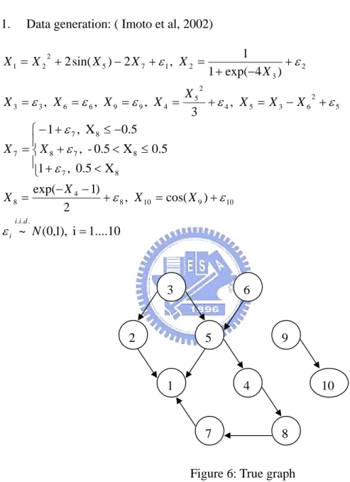
1. Data generation: ( Imoto et al, 2002)

1....10 i ), 1 , 0 ( ~ ) cos( , 2 ) 1 exp( X 0.5 , 1 5 . 0 X 0.5 , 5 . 0 X , 1 , 3 , , , ) 4 exp( 1 1 , 2 ) sin( 2 . . . 10 9 10 8 4 8 8 7 8 7 8 8 7 7 5 2 6 3 5 4 2 5 4 9 9 6 6 3 3 2 3 2 1 7 5 2 2 1 = + = + − − = ⎪ ⎩ ⎪ ⎨ ⎧ < + ≤ < + − ≤ + − = + − = + = = = = + − + = + − + = N X X X X X X X X X X X X X X X X X X X X d i i i ε ε ε ε ε ε ε ε ε ε ε ε ε 3 6 2 5 9 1 4 2. Analysis Methods:

Recall that the Cheng’s method (2003) only can find the causal effect direction but not the connected relation (repress or activate). Also, we discovered the threshold score of independence needs to be adjusted for different sample sizes. If we still use 0.9 as the threshold score, the graph size will be much larger than Figure 6 and there are too many

7 8

10

extra pathways. Also, the size of the resulting graph will be very large, and the Cheng’s method will lose its practicability. When the sample size is less than or equal to 100, we choose the threshold score of independence by considering the graph size of Figure 6. Therefore, the results of SCORE with the sample size less than 100 are adjusted. Table 6 is the threshold score of independence discovered in our simulation. (The threshold score will be used later in the real data analysis).

We modify Cheng’s method as described in the following: (1) Score evaluation is the same, S g(ˆ_λ)in (2.17).

(2) The threshold score (Table 6) changes with the sample size.

(3) Using the signs of the nonparametric correlation coefficients (Kendall’s Tau,

Spearman’s Rho) to indicate the way of connection (repress (-) or activate (+)).

(4) If one of the smoothing parameters is smaller than10−6, we replace it by

2 ) (λ₁ λ₂

λ_new = + , where λ₁andλ₂ are the smoothing parameters used in XÆY and YÆX, respectively.

We use “RANK” and “RANGE” to represent our methods with different pre-processing. Using “SCORE” represents the method modified Cheng’s method. We compare our proposed method (RANK and RANGE) with the modified Cheng’s method (SCORE).

We use different numbers of sample sizes (N) and the classes of ordinal type data (K) to see the performance of our methods and Cheng’s method.

Cheng (2003) has mentioned that if lambda (the smoothing parameter) is too small, then the fitting curve will be too rough. If lambda is too small, the influence of penalty term will be small. The curve will completely go with the data. This may cause the curve undersmooth. She also suggests that if one of the λ' s is smaller than10−6, it should be adjusted by a new lambda,

2 ) (λ1 λ2

are the smoothing parameters used in XÆY and YÆX, repectively. We take her idea and use

2 ) (λ1 λ2

λnew = + as our new lambda when the sample size is less than 100 and

lambda is smaller then10−6. 3. Simulation Results

(1) When the sample size (N) is less than 100, the graph size of SCORE is smaller than RANK and RANGE. The threshold values of independence of SCORE are given in Table 4. ( Figure 28~Figure 34)

(2) When N is larger than 100, the graph size of SCORE is larger than RANK and RANGE. The threshold limits of independence of SCORE we used are 0.9. (Figure 22~Figure 27)

(3) If we check the functions that generate the data, we can see that there are still some atavistic relationships between those variables. Figure 6 does not show this relation. RANK, RANGE, and SCORE can show some of these atavistic relations. We find that RANK and RANGE is more sensitive than SCORE with this kind of relation when the sample size is larger than 100.

decreases.

3

6

2

5

9

1

4

10

7

8

Figure 7: Figure 6 with some atavistic relationships

(4) The graph size of RANK and RANGE decreases as the sample size

of SCORE increases as the sample size decreases. When the sample size is less than 100, the graph size of SCORE grows very quickly as N decreases. (Figure 22 (A) Æ Figure 12 (A) Æ Figure 24 (A) Æ Figure 25 (A) Æ Figure 27 (A)Æ Figure 28 (B) Æ Figure 29 (B) Æ Figure 31 (B) Æ Figure 33 (B))

Check the results of RANGE and RANK. The number of wron

(5) g directions

ber of w sample s

(6)

when N≤100 (Table 4) is larger than that when N≥100 (Table 2). That is, the num rong directions increases when the ize decreases. For both RANK and RANGE methods, when N ≤100, the number of extra

100 ≥

(7) E without adjusting lambda, the number of missing pathways (Table 4) is smaller than that when N (Table 2). That is, the number of extra pathways decreases with the sample size decreases. The result of SCORE is opposite.

For RANK and RANG

pathways when N <100(Table 4) is not large. We find that it is not necessary to adjust lambda

(8) with RANK and RANGE. But

(9) NK and RANGE

it is necessary to adjust lambda with SCORE, especially when the sample size is less than 100. (Compare Figure 33 (A) with Figure 33 (B))

We find that there are still some relations not detected by RA

even if the sample size is large. The reason is that the first-step correlation test cannot detect some symmetrical functions. (For example, f x( )=x2. Details

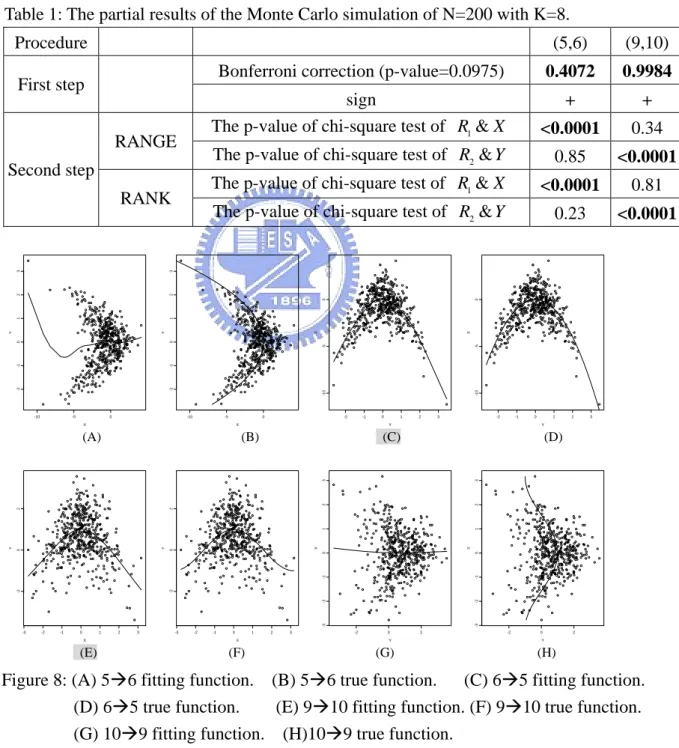
can be seen in Section 4.2.) Although we may not be ab ct those relationships in step one, we can adjust the result by the second step. If the functional structure between two variables is symmetrical and we cannot detect it from the first step, the p-value of chi-square test of one direction in the second step will be very close to zero, (e.g., <0.0001). We give the following example: Table 1 (partial result of Table 10) shows that the p-values of the first step are larger than 0.0975. Our method indicates that both (5, 6) and (9, 10)

have no strong relation. But Figure 8 shows that there is a relation between (5, 6) (Figure 8 (C)) and between (9, 10) (Figure 8 (E)). At the second step, the p-value of the chi-square test is about zero in one of the directions. We find that this condition indicates that some relations are missed and we must regulate the results of the step-one and change the conclusion to 6⎯⎯+→ and95 ⎯⎯+→ . 10

K=8. (From Table 2) N=200,

e Monte Carlo simulation of N=200 with K=8. Table 1: The partial results of th

Procedure (5,6) (9,10)

Bonferroni correction (p-value=0.0975) 0.4072 0.9984 First step

sign + +

The p-value of chi-square test of R1&X <0.0001 0.34

RANGE

2&

R Y <0.0001

The p-value of chi-square test of 0.85

The p-value of chi-square test of R1&X <0.0001 0.81

Second step

RANK

&

The p-value of chi-square test of R₂ Y 0.23 <0.0001

X Y -10 -5 0 -2 -1 0 1 2 3 X Y -10 -5 0 -2 -1 0 1 2 3 Y X -2 -1 0 1 2 3 -10 -5 0 Y X -2 -1 0 1 2 3 -10 -5 0 X Y -3 -2 -1 0 1 2 3 -2 0 2 X Y -3 -2 -1 0 1 2 3 -2 0 2 Y X -2 0 2 -3 -2 -1 0 1 2 3 Y X -2 0 2 -3 -2 -1 0 1 2 3 (A) (B) (C) (D) (F) (E) (G) (H)

Figure 8: (A) 5Æ6 fitting function. (B) 5Æ6 true function. (C) 6Æ5 fitting function.

Æ Æ Æ

(D) 6 5 true function. (E) 9 10 fitting function. (F) 9 10 true function.

Æ Æ

(10) The discovery of the threshold of SCORE from Table 6:

reases.

we use the

3. ting lambda is larger than that with

4.2 A study on Causal Relationships

,1), ~ (0,1), ~N(0,0.5). Functions:

, , , , sin( ) , .

The Sample size ( ) = 1000. X

N

Y e Y X Y X Y X Y X Y X

N

ε ε

1. The threshold value decreases when the sample size dec

2. The decreasing speed of the threshold value is slow, when SCORE method with adjusting lambda.

The graph size of SCORE without adjus lambda adjusted. 1. Data generation: 2 (0,1), X ~ (2 X N N 2 1/ 3 1/ 3 2 2 2 2 2 2 ~ ε ε − ε ε ε ε = + = + = + = + = + = +

2. Analysis Methods: RANK, RANGE, and SCORE.

method can detect the monotone functional structures. But if the 3. Results:

(1) Our

functions are symmetric, like 2

( )

f X =X , it is not easy to detect. But if we detect that there is a relation between those two variables, there is about 90% correct rate (see Table 9). We suggest not to use 2 as the number of classes of ordinal type data (Table 8 shows the accurate rate may decrease to 0.340/0.328).

We find that u

(2) sing 4 as the number of classes of the ordinal type data gets a

(3) n

better result compared with other number of classes (see Table 7 ~ Table 9). We can see that if we only consider two variables, SCORE will be better tha our methods (Compare Table 8 with Table 10). But if the number of variables is more than two and the sample size is small, our method will be better.

4.3 Real D

ycle measurements of Spellman et al. (1998) ata Analysis

1. Data source: S. cerevisiae cell-c

http://cell-cycle-www.standford.edu http://www.molbiolcell.org/

We use the data of the experiment CDC28. The data were collected at 17 different time

alysis Methods: The sample size is very small (N=17), we differentiate the

3. show some of the resulting gene network

(1) Case 1: points.

2. An

relations between genes by RANK, RANGE, and SCORE. We use 0.72 (from Table 6) as the threshold of SCORE.

Analysis results: In the following, we

YGP1

PDS1

FAR1

INH

NUF1

TEC1

+

+

-

-1

-Figure 9: A partial predicted gene regulatory network for the yeast data (CDC28) from Xu et al. (2002). This network is constructed not only by the Smooth Response Surface algorithm but also by the exiting biological knowledge.

raph size of RANK and RANGE are both 9 and equal to SCORE after being adju

using RAN

ith K = 4, without adjusting lambda, it is more similar to Figure 1 than

The g

sted. Their graph sizes are similar if we use 0.72 as the threshold of SCORE. We can see that the difference of adjusting lambda or not is small when

GE. Comparing with Figure 9, it seems that the number of wrong pathways are less with K = 2.

For RANK w

that with lambda adjusted (See Figure 18 (A) and Figure 18 (C)). But using RANK with K = 2 will do better with lambda adjusted (See Figure 18 (E) and Figure 18 (G)). This may be due to that the Yates' continuity correction will be applied when the

YGP1 PDS1 FAR1 INH1 NUF1 TEC1 + + + + + - + + - (B) YGP1 PDS1 FAR1 INH1 NUF1 TEC1 + + + + + - + + - (A) YGP1 PDS1 FAR1 INH1 NUF1 TEC1 + + + + + - +

Figure 11: The resulting network constructed by our methods. Figure1

Accurate direction

Wrong direction

Extra pathway

Missing pathway

- +

0: The resulting network constructed by SCORE The threshold of score is 0.72

(A) RANK with K=4 and without adjusting lambda. (B) RANGE with K=4 and without adjusting lambda.

expected cell counts of chi-square test are smaller than five. Chi-square test’s validity depends heavily on the assumption that the expected cell counts are at least moderately large; a minimum size of five is often quoted as a rule of thumb. In both RANK and RANGE, the number of two-way pathways is large with K = 2 (See Figure 18).

Case 2: HES1 FAA1 CPS1 HAP1 ARE2 CDC45 TOP3 RAD27 SMC1 + -- -+ + + +

A partial predicted gene re y network for the yeast ta (CDC28) +

Figure12: gulator da

from Xu et al (2002). This netwrok was not only constructed by Smooth Response Surface algorithm but also adjusted by the exiting biological knowledge.

HES1 FAA1 CPS1 HAP1 ARE2 CDC45 TOP3 RAD27 SMC1 - - + + + + + - - -

Accurate direction

Wrong direction

Extra pathway

Missing pathway

+ + - + + + -

Figure 13: The figure of SCORE when lambda adjusted. The threshold of score is 0.72 (from the Monte Carlo simulation).

In this case we can find that the graph size of SCORE is similar with that of RANK and RANGE. But if we use SCORE and do not adjust lambda (Figure 20 (A)), the graph size of SCORE will be larger than that of our methods. We find that using RANK and K=4 will do better when without adjusting the lambda, RANGE and K=4 will do better when lambda adjusted. There is no big difference when K=2 whether adjusting lambda or not. Summarizing the above results, RANK with K=4 is closer to Figure 12.

After checking these two cases, we find that RANK with K=4 and without adjusting the lambda is closer to Figure 9 and Figure12.

HES1 FAA1 CPS1 HAP1 ARE2 CDC45 TOP3 RAD27 SMC1 + + + + + + + ++ - - - - - - + + HES1 FAA1 CPS1 HAP1 ARE2 CDC45 TOP3 RAD27 SMC1

Accurate direction

Wrong direction

Extra pathway

Missing pathway

+ + - + + + - - - + + + + - + + -

Figure14: RANK with K=4 without adjusting lambda.

5. Discussions

The advantages of our method are we don’t need strong statistical assumption before using and compute rapidly. Especially when the sample size is small, the resulting graph size is still similar to the graph size of larger sample size. We give the following conclusions:

1. The method proposed by Cheng (2003) is not always proper for small sample sizes. We find that the threshold of independence need to be adjusted adapt to the sample size when sample size is smaller than 100. If we all use 0.9 for the threshold score and ignore the effect of the sample size, the graph size will grow quickly as the sample size decreases. We suggest that we should find the threshold score by simulation before starting the real data analysis. Table 4 gives the result of the threshold score from our simulation study.

2. If we only consider two variables, the method proposed by Cheng will be better than our method. If we need to identify the relevant connections between

sets of genes, our method will be better. When the threshold point is not

adjusted, the graph size of the result using the method proposed by Cheng will be a serious problem.

3. From simulation results, we can see that the resulting graph sizes of our method do not change acutely when the sample sizes are different.

4. There are some particular functional structures that can not be easily detected by our methods. For example, 2

( )

f x =x . The correlation test of the first step cannot detect some symmetrical functions. But we can adjust the result by the second step. If the functional structure between two variables is symmetrical and we cannot detect from the first step, the p-value of the chi-square test for

one direction at the second step will be very close to zero (<0.0001). The detail is showed in the Table 11.

5. Cheng (2003) has mentioned that if the lambda is too small, then the fitting curve will be too rough. If a lambda is smaller than 6

10− , it is adjusted to a new lambda such as 1 2

2 new

λ λ

λ = + or λ_new = λ λ_{1 2} . Our methods (RANK and RANGE) also use the nonparametric regression to estimate the curve. But we find that the magnitude of lambda has no big influence for our methods. If we ignore the small value of lambda and do not adjust the lambda, we still can discover the relations. Also, without adjusting lambda, we may get a better direction.

We consider the following problems as future works:

1. How to discretize the continuous data and not miss much of the information. 2. Use other correlation tests which are sensitive to the unusual points. We use

two nonparametric rank correlation tests that are both not sensitive to the unusual points. That may ignore the effect of influential points.

3. Our method is not sensitive with symmetric and linear functional structure. How to cope with this situation?

References

[1] Akutsu T, Kuhara S, Maruyama O, and Miyano S. (2003). “Identification of gene regulatory networks by strategic gene disruptions and gene overexpressions.”

Theor. Comput. Sci., 298, 235-251. (Preliminary version has appeared in Proc. 9th ACM-SIAM Symp. “Discrete Algorithms.” (1998), 56, 695-702.)

[2] Akutsu T, Miyano S, and Kuhara S. (1999). “Identification of genetic networks from a small number of gene expression patterns under the Boolean network model.” Pac. Symp. Biocomput., 4, 17-28.

[3] Akutsu T, Miyano S, Kuhara S. (2000). “Algorithms for identifying Boolean networks and related biological networks based on matrix multiplication and fingerprint function.” J Comput Biol., 7, 331-343.

[4] Akutsu T, Miyano S, Kuhara S. (2000). “Inferring qualitative relations in genetic networks and metabolic pathways.” Bioinformatics, 16(8), 727-734.

[5] Chakravarti, Laha, and Roy. (1967) Handbook of Methods of Applied Statistics. Volume I, John Wiley and Sons.

[6] Chen T, He HL, Church GM. (1999). “Modeling gene expression with differential equations.” Pac Symp Biocomput., 29-40.

[7] Cheng C Y. (2003). “Determining the Cause-Effect Relationship between Two Variables by Nonparametric Regression.” Master Thesis. Institute of Statistics, National Chiao-Tung University.

[8] Lu C H. (2003). “Determine the causal relationship between two variables.” Master Thesis. Instituteof Statistics, National Chiao-Tung University.

[9] De Hoon M J, Imoto S, Kobayashi K, Ogasawara N, Miyano S. (2003). “Inferring gene regulatory networks from time-ordered gene expression data of Bacillus subtilis using differential equations.” Pac Symp Biocomput., 17-28.

[10] Friedman N. and Goldszmidt M. (1998). Learning Bayesian Networks with local

Structure. Jordan, M.I. (ed.), Kluwer Academic Publisher.

[11] Friedman N, Linial M, Nachman I, Pe'er D. (2000). “Using Bayesian networks to analyze expression data.” J Comput Biol. 7(3-4), 601-620.

[12] Helsel D R and Hirsch R M. (1995). Statistical Methods in Water Resources,

Studies in Environmental Sciences 49. Elsevier, Amsterdam.

Publishing, Co., New York.

[14] Imoto S, Goto T and Miyano T. (2002). “Estimating of genetic networks and functional structures between genes by using Bayesian networks and nonparametric regression.” Proc. Pacific Symposium on Biocomputing, 7, 175-186. [15] Imoto S, Higuchi T, Goto T, Tashiro K, Kuhara S and Miyano S. (2003). “Combining Microarrays and Biological Knowledge for Estimating Gene Networks via Bayesian Networks.” Technical Report, Human Genome Center, Institute of Medical Science, University of Tokyo, Japan.

[16] Imoto S, SunYong K, Goto T, Aburatani A, Tashiro K, Kuhara S, and Miyano S. “Bayesian network and nonparametric heteroscedastic regression for nonlinear modeling of genetic network.” Journal of Bioinformatics and Computational

Biology, in press. (Preliminary version has appeared in Proc. IEEE Computer

Society Bioinformatics Conference.2002, 219-227.)

[17] Jeffrey S Simonoff. (1996). Smoothing Methods in Statistics. Springer series in statstics.

[18] Maki Y, Tominaga D, Okamoto M, Watanabe S, Eguchi Y. (2001) “Development of a system for the inference of large scale genetic networks.” Pac Symp Biocomput., 446-458.

[19] Pearl J. (2000). Causality: models, reasoning, and inference. Cambridge University Press, Cambridge, New York.

[20] Shmulevich I, Dougherty ER, Kim S, Zhang W. (2002). “Probabilistic Boolean Networks: a rule-based uncertainty model for gene regulatory networks.”

Bioinformatics, 18(2), 261-74.

[21] Sida´k Z. (1968). “On multivariate normal probabilities of rectangles: Their dependence on correlations.” Ann Math Statist., 39, 1425–1434.

[22] Sida´k Z. (1971). “On probabilities of rectangles in multivariate normal Student distributions: their dependence on correlations.” Ann Math Statist. 41, 169–175 [23] Siegel S and Castellan N J. (1988). Nonparametric Statistics.

[24] Siegel S. (1956). Nonparametric Statistics. McGraw-Hill. London.

[25] Snedecor, George W and Cochran, William G. (1989). Statistical methods. English Edition, Iowa Stat University Press.

Nonparametric Regression for Nonlinear Modeling of Gene Networks from Time Series Gene Expression Data.” Proc. 1st International Workshop on Computational Methods in System Biology. Lecture Note in Computer Science, 2602,

Springer-Verlag. 104-113.

[27] Tamada Y, Kim S, Bannai H, Imoto S, Tashiro K, Kuhara S, and Miyano S. (2003). “Estimating gene networks from gene expression data by combining Bayesian network model with promoter element detection.” Bioinformatics, 19 Suppl 2, II227-II236.

[28] Xu H, Wu P, Wu CF, Tidwell C, and Wang Y. (2002). “A smooth response surface algorithm for constructing a gene regulatory network.” Physiol Genomics, 11(1), 11-20.

Tables

Table 2: The summary of larger sample size. i.e., Figures of right below the described compared with Figure 6.

Sample size K Rank Rate/missing/extra/wrong Range Rate/missing/extra/wrong Score 1000 8 77.8~82.2%/2/6/2 Figure 22(B) 80~84.4%/2/6/1 Figure 22(C) 91%/0/2/2 Figure 22(A) 1000 8 80~82.2%/1/7/2 Figure 23(B) 82.2%~84.4%/1/7/1 Figure 23(C) 91%/2/1/1 Figure 23(A) 500 8 80%/0/7/2 Figure 24(B) 80%/0/7/2 Figure 24(C) 91%/0/3/2 Figure 24(A) 8 80%/2/7/2 Figure 25(B) 80%/2/7/2 Figure 25(C) 200

4 84.4%/2/6/0 Figure 25(D) 84.4%/2/6/0 Figure 25(E)

88.9%/0/3/2 Figure 25(A)

8 82.2%/3/4/1 Figure 26(B) 80%/3/4/2 Figure 26(C)

100

4 80%/3/4/2 Figure 26(D) 75.6%/3/4/4 Figure 26(E)

86.7%/1/3/2 S=0.9 Figure 26(A) 65%/1/12/3 S=0.9 Figure 27(A) 100 8 75.6%/3/6/2 Figure 27(C) 77.8%/3/6/1 Figure 27(D) 84.4%/1/4/2 S2=0.73 Figure 27(B)

K: the number of class of ordinal data.