國立臺中教育大學資訊工程學系碩士論文
高效能計算即服務平台上於執行期限條
件下以收益極大化為目標之可調式平行
工作排程方法研究
Revenue Maximization for Scheduling
Deadline-Constrained Moldable Jobs on High
Performance Computing as a Service Platforms
指導教授:黃國展 博士
研究生:洪俊豪 撰
致謝
謝謝老師兩年來的用心指導和照顧,讓我有機會學習研究和實作一個不小的系統, 在實作那個系統的過程當中,我也學到了不少如何做 jar 的 library,並且將系統寫得很 有彈性,能夠當作 library 給別人使用。還有我也練習了不少如何將其他程式轉成我們平 台的架構,對於程式碼的轉換更加的熟悉。研究方面,我也學到如何從一開始瀏覽人家 的研究成功,從中找出可能可以改善的地方,進而發展自己的演算法,實驗,和發表與 報告,也讓我練習了不少次的報告,讓我在報告的時候不會容易緊張而忘記要報告的內 容。 我也要謝謝來問我問題的同學,它讓我學到一些其他領域的東西,還有就是熟悉 C 的 byte 操作,這個部分之前我比較少接觸,因此其實不是太熟悉這個操作。 謝謝父母願意讓我讀研究所,能夠讓我學得更多。摘要
傳統的高效能計算系統所處理的工作型態通常稱為「盡力就好」類型,因為這些工 作通常沒有執行完成期限的要求,系統排程的原則僅是愈快愈好。最近「高效能計算即 服務」的概念被提出,主要目的就是希望讓高效能計算的設備和應用以一種便捷的服務 模式來提供給使用者採用。為了達到這個目標,我們將面臨新形態的工作排程議題,例 如處理帶有執行期限的工作及嘗試讓服務提供者的獲利極大化等。這篇論文提出一個以 預留資源為基礎的動態工作排程方法,來處理未來高效能計算即服務平台上帶有執行期 限要求之可調式平行工作的排程議題,目標是要極大化服務提供者的收益。我們執行了 一系列的模擬實驗來評估所提出的這個排程方法並與文獻中的先前方法進行比較。實驗 結果顯示我們的排程方法能夠有效地進一步提升服務提供者的收益。在實驗中我們也探 討了幾項相關的議題,包括工作等待貯列內的優先權擇定、時間上及空間上的處理器配 置原則、及計費模式等。 關鍵字: 可調式平行工作、排程、有完成期限限制的工作、高效能運算、收入極大化、 處理器配置Abstract
Traditionally, High-Performance Computing (HPC) systems usually deal with the so called best-effort jobs which do not have deadline and are scheduled in an as-quick-as-possible manner. Recently the concept of HPC as a Service (HPCaaS) was proposed, aiming to transforming HPC facilities and applications into a more convenient and accessible service model. To achieve that goal, there will be new focuses and issues to explore, such as scheduling jobs with deadline and maximizing the revenue of service providers. This thesis presents a reservation-based dynamic scheduling approach for efficiently scheduling deadline-constrained moldable jobs with the aim of maximizing a service provider’s revenue. The proposed approach was evaluated with a series of simulation experiments. The experimental results indicate that our job scheduling approach can achieve higher revenue than previous methods. In the experiments, we also explored several related issues, such as waiting queue sequencing, processor allocation decisions on time and space, charge model.
Keywords: moldable jobs, scheduling, deadline-constrained jobs, high performance
Table of Contents
致謝 ... II
摘要 ...III
Abstract ... IV
Table of Contents ... V
List of Figure ... VI
Chapter 1. Introduction ... 1
Chapter 2. Related Work ... 4
Chapter 3. Scheduling Deadline-Constrained Moldable Jobs for Revenue
Maximization ... 8
Chapter 4. Simulation Environment ... 14
Chapter 5. Performance Evaluation ... 20
Chapter 6. Conclusions ... 43
List of Figure
Fig. 2.1. Classification of parallel job scheduling research ... 4
Fig. 3.1 Partial schedule represented by a profile ... 10
Fig. 4.1: Graphic user interface for FPJS
2E
2... 15
Fig. 4.2: Simulation configuration with a configuration file ... 15
Fig. 4.3: Direct simulation configuration without configuration file... 16
Fig 4.4: Simulation result ... 16
Fig. 4.5: Class diagram for basic components in FPJS
2E
2... 18
Fig. 4.6: Class for our Simulation... 19
Fig. 5.1 Penalty for soft-deadline jobs with sequential-runtime charge
model and SJF policy ... 24
Fig. 5.2 Profit for soft-deadline jobs with sequential-runtime charge
model and SJF policy ... 25
Fig. 5.3 Penalty for soft-deadline jobs with sequential-runtime charge
model and ASAP+AFAP policy ... 25
Fig. 5.4 Profit for soft-deadline jobs with sequential-runtime charge
model and ASAP+AFAP policy ... 25
Fig. 5.5 Average turnaround time for soft-deadline jobs with
sequential-runtime charge model and ASAP+AFAP policy... 26
Fig. 5.6 Penalty for soft-deadline jobs with parallel-runtime charge model
and SJF policy ... 26
Fig. 5.7 Profit for soft-deadline jobs with parallel-runtime charge model
and SJF policy ... 26
Fig.
5.8
Deadline
miss
rate
for
hard-deadline
jobs
with
sequential-runtime charge model and the EDF policy ... 27
Fig. 5.9 Completion rate for hard-deadline jobs with sequential-runtime
charge model and the EDF policy ... 28
Fig. 5.10 Penalty for hard-deadline jobs with sequential-runtime charge
model and the EDF policy ... 28
Fig. 5.11 Income for hard-deadline jobs with sequential-runtime charge
model and the EDF policy ... 28
Fig. 5.12 Profit for hard-deadline jobs with sequential-runtime charge
model and the EDF policy ... 29
Fig. 5.13 An example with ALAP ... 29
Fig. 5.14 An example with ASAP ... 29
Table 5.1 Job attributes and miss counts ... 30
Fig.
5.15
Deadline
miss
rate
for
hard-deadline
jobs
with
sequential-runtime charge model and ALAP+AFAP policy ... 31
Fig. 5.16 Completion rate for hard-deadline jobs with sequential-runtime
charge model and ALAP+AFAP policy ... 31
Fig. 5.17 Profit for hard-deadline jobs with sequential-runtime charge
model and ALAP+AFAP policy ... 31
Fig. 5.18 Deadline miss rate for hard-deadline jobs with parallel-runtime
charge model and the LIF policy... 32
Fig. 5.19 Completion rate for hard-deadline jobs with parallel-runtime
charge model and the LIF policy... 32
Fig. 5.20 Penalty for hard-deadline jobs with parallel-runtime charge
model and the LIF policy ... 32
Fig. 5.21 Income for hard-deadline jobs with parallel-runtime charge
model and the LIF policy ... 33
Fig. 5.22 Profit for hard-deadline jobs with parallel-runtime charge
model and the LIF policy ... 33
Fig. 5.23 Deadline miss rate for hard-deadline jobs with parallel-runtime
charge model and the ALAP+AMAP policy ... 34
Fig. 5.24 Completion rate for hard-deadline jobs with parallel-runtime
charge model and the ALAP+AMAP policy ... 34
Fig. 5.25 Penalty for hard-deadline jobs with parallel-runtime charge
model and the ALAP+AMAP policy ... 34
Fig. 5.26 Income for hard-deadline jobs with parallel-runtime charge
model and the ALAP+AMAP policy ... 35
Fig. 5.27 Profit for hard-deadline jobs with parallel-runtime charge
model and the ALAP+AMAP policy ... 35
Fig. 5.28 Comparing different methods by penalty for hard-deadline jobs
with the sequential-runtime charge model ... 36
Fig. 5.29 Comparing different methods by income for hard-deadline jobs
with the sequential-runtime charge model ... 36
Fig. 5.30 Comparing different methods by profit for hard-deadline jobs
with the sequential-runtime charge model ... 37
Fig. 5.31 Comparing different methods by penalty for hard-deadline jobs
with the parallel-runtime charge model ... 37
Fig. 5.32 Comparing different methods by income for hard-deadline jobs
with the parallel-runtime charge model ... 38
Fig. 5.33 Comparing different methods by profit for hard-deadline jobs
with the parallel-runtime charge model ... 38
Fig. 5.34 Comparison of scheduling overhead of different methods ... 39
Fig. 5.35 Evaluation of deadline-miss rate for partial re-scheduling in
hard-deadline scenarios with the sequential-runtime charge model ... 40
Fig. 5.36 Evaluation of completion rate for partial re-scheduling in
hard-deadline scenarios with the sequential-runtime charge model ... 40
Fig. 5.37 Evaluation of profit for partial re-scheduling in hard-deadline
scenarios with the sequential-runtime charge model ... 41
Fig. 5.38 Evaluation of deadline-miss rate for partial re-scheduling in
hard-deadline scenarios with the parallel-runtime charge model ... 41
Fig. 5.39 Evaluation of completion rate for partial re-scheduling in
hard-deadline scenarios with the parallel-runtime charge model ... 41
Fig. 5.40 Evaluation of profit for partial re-scheduling in hard-deadline
scenarios with the parallel-runtime charge model ... 42
Chapter 1. Introduction
High performance computing (HPC) has long been a very important field for solving large-scale complex scientific and engineering problems. However, accessing and running applications on HPC systems remains tedious, limiting wider adoption and user population [1]. As cloud computing [2] emerges, which emphasizes easier and efficient access to IT infrastructure, recently the concept of HPC as a Service (HPCaaS) [1] was proposed to transform HPC facilities and applications into a more convenient and accessible service model.
Traditionally, HPC systems usually deal with the so called best-effort jobs which do not have deadline and are scheduled and executed in an as-quick-as-possible manner. Various scheduling methods have been developed to optimize the average (weighted) turnaround time of all jobs in the system [3][4][5]. However, as HPC turns into the service model, there will be new types of jobs appearing on HPCaaS platforms, such as jobs with deadline. Moreover, as a kind of paid services, it’s natural that new focuses of job scheduling might appear in addition to the traditional goal of minimizing average turnaround time of all jobs. For example, it’s very likely that the service providers of HPCaaS would tend to maximize their revenues by applying appropriate job scheduling approaches. Therefore, there are emerging scheduling issues to explore for dealing with the new focuses and new types of jobs on HPCaaS platforms. This thesis presents a reservation-based dynamic scheduling approach for efficiently scheduling deadline-constrained moldable jobs with the aim of maximizing a service provider’s revenue.
Parallel jobs, according to their flexibility in parallelism, can be classified into four types [6]: (1) Rigid, (2) Moldable (3) Evolving, and (4) Malleable. A rigid job [6] can only run with a specific number of processors specified by users upon job submission. Moldable jobs [6] are
flexible in the number of processors to use at the time a job starts, but the number of processors cannot be changed during execution. Malleable and evolving jobs [6] are similar to moldable jobs in that they all have the potential to run with different parallelisms in contrast to rigid jobs. However, malleable and evolving jobs are even more flexible in that they can change the amount of processors used dynamically during execution. While both evolving and malleable jobs can change their processor requirements during execution, for evolving jobs the change is application initiated, but the change in malleable jobs is system initiated. Since most modern parallel application programs can be elaborately designed to have the moldable property, such as the famous HPC benchmark program HPL [7] and other parallel applications written in MPI [8], in this thesis we focus on scheduling moldable jobs in HPCaaS systems.
There have been many research works in the literature [9][10][11][12] dealing with scheduling rigid jobs with deadline. However, few works have been done for scheduling moldable jobs with deadline. For moldable jobs, the flexibility in parallelism opens new possibilities and raises new issues for scheduling jobs to meet their deadlines. This thesis deals with such issues and develops a new scheduling approach for online scheduling of deadline-constrained moldable jobs with the aim of maximizing HPCaaS providers’ revenues. Three important issues were explored when designing the scheduling approach. The first is concerned with the waiting queue sequencing policy. The second is related to processor allocation decisions on time and space. The third issue is about the charge model for running deadline-constrained moldable jobs on HPCaaS platforms. The proposed approach has been evaluated with a series of simulation experiments and and compared to two previous methods, moldable EDF in [27] and Algorithm 3 in [35], based on a publically available workload log [13].
The reminder of this thesis is organized as follows. Section 2 discusses related works on parallel job scheduling. We present our moldable job scheduling approach in section 3. Section 4 presents the architecture of our simulation environment. Section 5 evaluates and compares the proposed approach in terms of various performance metrics through a series of simulation experiments. Section 5 concludes this thesis.
Chapter 2. Related Work
In [1], AbdelBaky et al. proposed the concept of HPC as a Service, aiming to transform traditional HPC resources into a more convenient and accessible service. They focused on the issues related to elastic provisioning and dynamic scalability, which are concerned in malleable jobs [6]. In this thesis, we focus on the moldable property [6] in most modern parallel applications. Most existing HPC systems usually treat parallel jobs as rigid and require that users specify the amount of processors to use when submitting jobs, even though the parallel jobs have the moldable property. According to treating parallel jobs as rigid or moldable, and whether a job has a deadline or not, we divide most of the research works on parallel job scheduling into the four quadrants as shown in Figure 2.1.
Fig. 2.1. Classification of parallel job scheduling research
Scheduling rigid jobs without deadline, quadrant I, has long been an important research field in high-performance computing and parallel processing. Many research efforts have been spent on developing backfilling job scheduling approaches for resolving the resource fragmentation issues under the FCFS policy [14][15][16][17]. The authors of [15] proposed an EASY-backfilling approach where a job can bypass other jobs with earlier arrival time than it provided that such bypassing would not delay the expected start time of the first job in the
Rigid Moldable no
deadline I II deadline III IV
waiting queue. The work in [16] investigates the impact of under-estimation of job execution time on the performance of the EASY-backfilling approach. Various backfilling scheduling approaches are compared and evaluated in [14].
For moldable jobs without deadline, quadrant II, previous research [18] has shown potential performance improvement achieved by adaptive processor allocation. The proposed adaptive processor allocation methods in [18] dynamically determine the number of processors to allocate just before job execution according to the amount of currently available resources and job queue information. In [19][20], Srinivasan et al. proposed a schedule-time aggressive fair-share strategy for moldable jobs, which adopts a profile-based allocation scheme. This strategy thus needs to have the knowledge of job execution time.
Scheduling jobs with deadline is an important issue in many fields, such as real-time systems, and thus there are many research works in the literature discussing related problems [21][22][23][32][37]. Earliest-Deadline-First (EDF) has been one of the most commonly used heuristics for scheduling jobs with deadline. In [24] EDF was applied to maintain timeliness and data freshness while minimizing imposed workload in real-time database research. In [38] EDF has been applied to scheduling real-time tasks on multicore processors. Another popular heuristic, called Least-Laxity-First (LLF), was used in [23] for scheduling jobs with deadline in distributed systems. For moldable jobs, it is hard to apply the LLF heuristic since the required execution time of a moldable job depends on the amount of processors used and thus is not a fixed value available for calculating the laxity.
The work in [21] presents algorithms with priority strategies for scheduling sequential tasks on a network enabled server (NES) environment. Many scheduling approaches concerning deadline in real-time systems were reviewed and compared in [25], including EDF,
LLF, and Rate-Monotonic algorithms. As cloud computing emerges, some research works, such as [22][26], begin to consider the scheduling issues of tasks with deadline constraints in cloud environments. In [22], an adaptive resource management policy was proposed to handle requests of deadline-bound applications with elastic clouds. The work in [26] addresses the problem of remote scheduling of a periodic and sporadic tasks with deadline constraints in cloud environments. In this thesis, we deal with scheduling online moldable jobs with deadline in HPCaaS environments.
As parallel job scheduling is concerned, most of the related work on deadline-constrained jobs deals with rigid jobs, quadrant III. Few attention has been paid on moldable jobs with deadline. In [27], Saule et al. proposed a moldable EDF method to schedule parallel jobs with deadline using the well-known Earliest Deadline First (EDF) heuristic. However, deadline is not the focus in [27] and the moldable EDF method was actually proposed to deal with optimizing the stretch of moldable jobs without deadline.
In [28], Ligang et al. addressed the problem of dynamically scheduling moldable jobs with QoS demands in multi-clusters. The QoS demand concerned in [28] is soft-deadlines. In addition to soft-deadlines, our work in this thesis also deals with jobs concerning hard-deadlines. In [29], Kwon et al. considered the problem of scheduling independent parallel tasks with individual deadlines so as to maximize the total work performed by the tasks which complete their executions before deadlines. The work deals with static scheduling and the speedup model of parallel jobs is assumed to be linear, while our work is for dynamic scheduling in HPCaaS environments and the speedup of a job with different numbers of processors is calculated using Amdahl’s Law [34].
In our previous work [35], three dynamic scheduling methods were proposed for deadline-constrained moldable jobs, aiming to minimize the deadline-miss rate. In the work of this thesis, we have developed a reservation-based dynamic scheduling approach, which can further improve the overall system performance, and the goal is to maximize HPCaaS providers’ profits instead of minimizing deadline-miss rate.
Chapter 3. Scheduling Deadline-Constrained
Moldable Jobs for Revenue Maximization
The three dynamic scheduling methods in [35] are based on the Earliest Deadline First (EDF) heuristic [25], but differ in how they handle the jobs in queue if the first job cannot meet the deadline with currently available processors. For all the three methods, when jobs are submitted to the system, they are inserted into the waiting queue in a non-decreasing order of their deadlines. The job scheduler is triggered by two kinds of events: job arrival and job finish. Upon each event, it repeatedly tries to allocate jobs for immediate execution according to the sequence in the waiting queue until no more jobs can be allocated. Each time the scheduler gets the first job in the waiting queue, which has the earliest deadline among all jobs. The scheduler then checks whether the first job can meet its deadline with currently available processors or not. If not, the scheduler can take different actions to deal with the situation, leading to the three different scheduling methods in [35].
In this section, we present a reservation-based dynamic scheduling approach, which differs from the three methods of [35] in that at each scheduling activity, in addition to allocating some jobs for immediate execution the scheduler also tries to make resource reservation for other jobs’ future execution. With the reservation mechanism, the proposed approach is expected to produce better schedules than previous methods. To implement the resource reservation mechanism, the proposed scheduling approach maintains a profile of the expected processor usage at future times. As described in [30], it is most convenient to maintain the profile in a linked list, as it may be necessary to split items into two when a newly scheduled
job is expected to terminate in the middle of a given period. In addition, an item may have to be added at the end of the profile whenever a job extends beyond the current end of the profile. The length of the profile is therefore proportional to the number of jobs running or in the waiting queue because each job adds at most one item to the profile.
In this study, we assume that the information of required execution time of a moldable job with different number of processors is available. Such assumption is common in research work of parallel job scheduling, such as [14][15][17]. Moreover, some research work has developed mechanisms for systems to automatically generate execution time predictions of jobs [31]. In addition, jobs are assumed not to be preempted or suspended once their execution starts. Each job is moldable and has a deadline specified by the user upon job submission.
The profile maintained by the reservation-based dynamic scheduling approach can be used to build the partial schedule of current jobs, running or waiting in the queue, as shown in Figure 3.1. In general, the proposed approach is a reservation-based dynamic scheduling framework for deadline-constrained moldable jobs, consisting of three important scheduling and allocation decisions to be made. The first is about the waiting queue sequencing policy, which determines the priority of each job for processor allocation. We will evaluate three possible policies in chapter 5, including Earliest Deadline First (EDF) [25], Shortest Job First (SJF) [33], and Largest Income First (LIF). The other two decisions are concerned with processor allocation, dealing with spatial and temporal allocation, respectively. As shown in Figure 3.1, there might be several time instants when the number of free processors changes in the partial schedule. The decision of temporal allocation determines how to select a time instant for a job to start execution, and the decision of spatial allocation is concerned with how many processors to be allocated to a job. We have developed As Soon As Possible (ASAP) and As Late As Possible
(ALAP) policies for temporal allocation, and As Few As Possible (AFAP) and As Many As Possible (AMAP) policies for spatial allocation. These polices will be evaluated in chapter 5.
Fig. 3.1 Partial schedule represented by a profile
Algorithm 1 in the following describes the framework of the reservation-based dynamic scheduling approach for deadline-constrained moldable jobs. The approach maintains a profile of the expected processor usage at future times for recording resource reservation, and is triggered by two types of events: job arrival and job finish. A job-arrival event occurs when a user submits a new job into the waiting queue, while a job-finish event indicates that some running job finishes its execution and releases the resources used by it. Upon receiving an event, the scheduler first checks the type of the event. If it is a job-arrival event, the scheduler inserts the new job into the waiting queue according to the pre-configured waiting queue sequencing policy, e.g. EDF, SJF (line 2). After the new job is inserted into some position in the waiting queue, the scheduler will update profile to clear the resource reservations for those jobs behind the new job, preparing for partial re-scheduling (lines 3 to 4). The partial re-scheduling process is described in lines 5 to 16. The scheduler tries to reserve enough resources in the future for each job behind the new job (line 5) to meet its deadline. The scheduler first tries each time instant in the profile (line 7), when the number of free processors changes, in a sequence according to the pre-configured temporal allocation policy, e.g. ASAP or ALAP. For each time
instant, the scheduler checks each possible number of processors under the constraint of free processors at that moment (line 8) in a sequence according to the pre-configured spatial allocation policy, e.g. AFAP or AMAP, to see whether there is a number of free processors for the job to start at the time instant and can finish its execution by its deadline. If such a time instant and an enough amount of free processors are found, the scheduler updates the profile to reserve the resources for the job (line 10). If no appropriate time instant can be found for a job to meet its deadline after checking the entire profile, the job will be marked as missing deadline (line 16). A job having no resource reservation will be removed from the waiting queue when current time proceeds to its deadline (lines 20 to 22). Only the scheduling activities triggered by a job-arrival event will go through lines 2 to 16. On the other hand, scheduling activities triggered by both types of events will conduct lines 17 to 22, starting execution of the jobs which have resource reservations starting from current time in the profile, and checking whether a job already misses its deadline. When the approach is applied to soft-deadline scenarios, once a job cannot find any time instant for resource reservation to meet its deadline, the scheduler will find a time instant and an amount of free processors that would lead to the least over-deadline time period for the job’s resource reservation.
Algorithm 1
Reservation-Based Dynamic Scheduling
Variables:
NP: number of free processors at the time instant checked;
Profile: a linked list recording future resource reservation for jobs in the waiting queue; Reserved: a boolean variable indicating whether a job
has successfully reserved enough resources for future execution;
1 If (the triggering event is job arrival)
begin
2 Insert the new job into the waiting queue according to the configured waiting queue sequencing policy;
3 index = the index of the new job in waiting queue; 4 Update profile to clear the resource reservations
for those jobs with indices larger than index; 5 for (i=index ; i<LengthOfWaitingQueue ; i++) begin
6 Reserved := false;
7 foreach (time instant in profile according to the configured temporal allocation policy) begin
8 foreach (number of processors less than or equal to NP)
begin
9 If (the job of index i can meet its deadline by starting at the time
instant with the number of processors) begin
10 Update profile to make resource reservation for the job;
11 Reserved := true; 12 break; end if end foreach 13 If (Reserved == true) begin 14 break; end if end foreach 15 If (Reserved == false) begin
16 mark the job of index i as missing deadline;
end if
end for end if
17 get the resource reservations in profile which start from current time; 18 foreach (reservations starting from current time)
begin
19 start the job with the amount of resources reserved for it;
end foreach
20 for ((i=0 ; i<LengthOfWaitingQueue ; i++)
begin
21 if (job of index i is marked as missing deadline and current time >= its deadline)
begin
22 remove the job of index i from the waiting queue; end if
Chapter 4. Simulation Environment
In order to conduct experiments for evaluating the proposed approach and comparing it with previous methods, we developed a software simulator in Java based on the discrete-event simulation methodology [36]. The simulator maintains a global clock, and the behavior of the simulated system is represented as a chronological sequence of events. The simulator runs in a loop to remove the smallest time-stamped event from the event queue and process it. Processing of an event would set the global clock to the time-stamp of the event, and might generate some new events. The simulator can be configured to call different scheduling algorithms to schedule the online parallel jobs.
The simulator is called a Flexible Parallel Job Scheduling Simulation and Evaluation Environment (FPJS2E2) with the aim of providing a convenient simulation and performance evaluation environment for researchers to evaluate and compare different parallel job scheduling methods. It is expected that based on the architecture and basic implementation of FPJS2E2, each researcher only needs to implement and replace one or two new classes for his own scheduling algorithm before he can start the experiments. This will save a lot of time for researchers because they don’t need to implement a whole new simulation program every time wanting to evaluate a new scheduling algorithm.
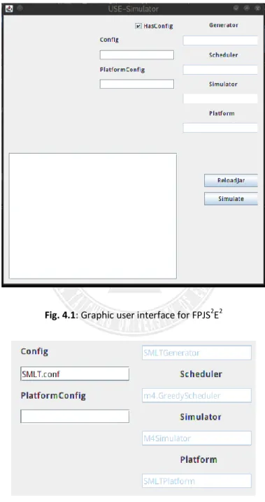
The main graphic user interface of FPJS2E2 is shown in Figure 4.1. There are two ways for setting up a simulation configuration before experiments. The first is with a configuration file as shown in Figure 4.2. The second way, as shown in Figure 4.3, is to un-check the “HasConfig” checkbox and directly input the simulation parameters in the user interface. When you finish the simulation configuration, pressing the “Simulate” button below will make the simulator
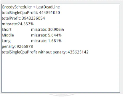
start the simulation of job scheduling and execution based on the classes you specify. After the simulation is completed, the experimental results will be displayed on the user interface, as shown in Figure 4.4.
Fig. 4.1: Graphic user interface for FPJS2E2
Fig. 4.3: Direct simulation configuration without configuration file
Fig 4.4: Simulation result
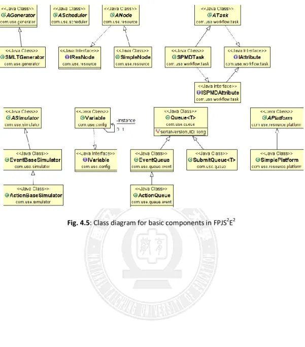
Figure 4.5 shows the class diagram of current implementation of FPJS2E2. The simulator has three essential components. The first is the class ASimulator encapsulating the main simulation program. Because different scheduling algorithms might need different simulation processes, we provide three member functions in ASimulator, including Initilize, simulateLoop, and simlateFinish, and other attributes for researchers to flexibly customize a simulation process suitable for their experiments. The function Initilized is for any initialization required for a simulation. The function simulateLoop implements the main
simulation loop for simulation progress. The function simulateFinish is for displaying the simulation results. This class also provides customized functions, println and print, allowing the output messages to be shown on either GUI or CLI. If you use the default print function to display messages, it won’t be shown on the GUI.
The second essential class is “Ascheduler”. The objective of this abstract class is to provide the schedule function to call during the simulation, as well as some other common functions and attributes. The third essential class is AGenerator, which provides the function generate generating the input workload, consisting of a set of parallel jobs or workflows. The function generate should be called in the Initilize function of ASimulator.
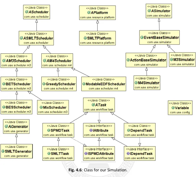
Current implementation of FPJS2E2 also provides some other classes you might need when developing your simulation experiments. Class APlatform implements the computing resources used in the simulation experiments. For example, the computing resources used in the experiments presented in this thesis is a cluster contains 128 processors. Figure 4.6 shows the class diagram that implement the scheduling algorithms presented and evaluated in this thesis.
Fig. 4.6: Class for our Simulation.
Chapter 5. Performance Evaluation
This section evaluates the proposed reservation-based dynamic scheduling approach, and compares it to two previous methods: the moldable EDF method in [27] and the Algorithm 3 in [35]. One thing to be noted is that moldable EDF was not developed for dynamic scheduling and the EDF + ASAP + AFAP combination in our reservation-based dynamic scheduling framework actually is the dynamic version of moldable EDF.
Since our goal is revenue maximization, to conduct the evaluation we have to define the profit model, charge model and penalty model first. The profit of an HPCaaS provider is defined to be the income minus the penalty. The income is determined by the charge model. In traditional HPC systems dealing with rigid jobs, the number of processors used to run a job is specified by the user, and thus the cost of running a job is simple to calculate, usually proportional to the number of processors used multiplied by the job’s parallel runtime, i.e. the period of wall-clock time that the processors are occupied. However, for dealing with moldable jobs where the number processors used is determined by the scheduler, not the user, there is not yet a commonly adopted charge model. One of the complexities comes from the fact that if the traditional charge model is used, using different numbers of processors for a job might lead to different costs since the efficiency of parallel applications usually is not 100%. Although using more processors usually leads to shorter turnaround time for a job, it also costs much. Therefore, an HPCaaS provider might tend to use more processors for a job to maximize its income, which could be unfair from the point of view of users. Since there is not a commonly agreed charge model for moldable jobs yet, in this study we evaluated the proposed scheduling approach with two possible charge model. The first model, called parallel-runtime model, is similar to the
traditional charge model where the fee of running a job is proportional to the number of processors used multiplied by the job’s parallel runtime. In the second model, called sequential-runtime model, the cost of running a job is determined by its equivalent sequential runtime, i.e. the execution time when running with one processor. We assume a job’s sequential runtime is available by the execution-time conversion based on the parallel speedup model, e.g. the Amdahl’s Law model [34].
For the penalty model, in the evaluation, we explored two types of deadline-constrained jobs: soft-deadline and hard-deadline. In the scenario of soft-deadline jobs, all jobs submitted will be executed. Some of them might meet their deadlines, while the others miss the deadlines. No penalty will be attributed to the jobs meeting their deadlines, and the penalty of a job missing its deadline is defined to be its finish time minus its deadline. For the scenario of hard-deadline jobs, the jobs missing their deadlines are further divided into two groups. The first group contains the jobs which are found to be unable to meet their deadlines right on their submission. Those jobs are viewed as being rejected immediately after their submission, and thus no penalties are assumed for them. The HPCaaS provider only loses some potential incomes. On the other hand, the second group of jobs are those that are found to be unable to meet their deadlines after a time period from their submission, due to the partial re-scheduling triggered by a new job’s arrival. The second group of jobs will account for penalties determined by their equivalent sequential runtime. Therefore, for the second group of jobs, the HPCaaS provider not only loses some potential incomes, but also pays for the penalties.
The experiments simulate a 128-processor homogeneous cluster and an online workload based on a public workload log [13]. The workload log contains 73496 records collected on a 128-node IBM SP2 machine at San Diego Supercomputer Center (SDSC) from May 1998 to
April 2000. After excluding some problematic records based on the completed field [13] in the log, the simulation experiments in this thesis use 56490 job records as the input workload. The speedup of a job with different numbers of processors is calculated using Amdahl’s Law [34]. The parameter α indicates the fraction of computation within a job that is parallelizable in Amdahl’s Law [34]. We set α=0.6 in the following experiments. The deadline of each job is given according to the following formula.
D(i) = Tsub(i) + k * Texec(1,i)
where i is the index of jobs; Tsub(i) is the submission time of job i; Texec(n,i) is execution time of job i with n processors; k is a random number picked up within a specified range, 0.1 to kmax. In the following experiments, kmax is set to 2.
In the following experiments, we evaluated three different waiting queue sequencing policies. The first is Earliest Deadline First (EDF) [25], where jobs with earlier deadline have higher priority. The second policy is Shortest Job First (SJF) [33], where jobs with shorter sequential runtime have higher priority. In contrast to SJF, the third policy, Largest Income First (LIF), tends to give higher priority to the jobs with longer sequential runtime since they are likely to bring more incomes.
For the temporal allocation policies, we evaluated As Soon As Possible (ASAP) and As Late As Possible (ALAP). With the ASAP policy, the scheduler will check the resource reservation profile in a non-decreasing order of time from the earliest time instant. On the other hand, for the ALAP policy, the scheduler starts from the latest time instant in the profile, and then proceeds in a non-increasing order of time.
For the spatial allocation policies, As Few As Possible (AFAP) and As Many As Possible (AMAP) were evaluated in the experiments. With AFAP, the scheduler tries to find a feasible amount of processor allocation at a specific time instant in the profile for a job to meet its deadline in an increasing order starting from one. On the other hand, for AMAP, the schedulers checks the possible amount of processor allocation in a decreasing order starting from a pre-defined threshold value. The threshold value is set to prevent the system from being trapped into a purely serial execution scenario where the jobs are executed one by one with each job exclusively using all processors in the system. As indicated by the Amdahl’s Law [34], efficiency of a parallel application usually declines as the number of used processors increases. Therefore, the purely serial execution scenario would lead to poor overall system performance, and should be avoided.
The proposed approach was evaluated and compared to previous methods in terms of different performance metrics, including deadline-miss rate, completion rate, average turnaround time, penalty, income, and profit, in different scenarios. Among them, completion rate is defined as the ratio of the amount of jobs meeting their deadlines over the total number of jobs submitted to the system. The deadline-miss rate is defined to be the number of jobs unable to meet their deadlines and incurring penalties divided by the total number of jobs submitted. Average turnaround time is one of the most commonly used performance metrics for comparing different batch job scheduling approaches, where turnaround time is calculated by subtracting the job submission time from the job finish time.
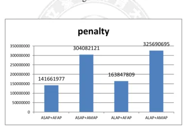
Figures 5.1 and 5.2 are representative experimental results comparing the different combinations of temporal and spatial allocation policies of the reservation-based dynamic scheduling approach with the sequential-runtime charge model. For waiting queue sequencing,
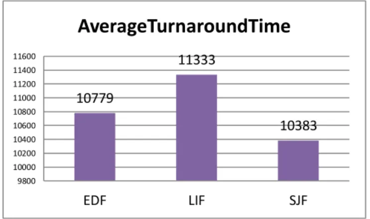
SJF was used in this scenario. For soft-deadline scenarios, all jobs will be executed, and thus the incomes of different methods are equivalent. Therefore, the profit is determined by the incurred penalty. Less penalties imply higher profits. The experimental results indicate that ASAP+AFAP leads to the largest profit. Figures 5.3 and 5.4 compare different waiting queue sequencing policies, using the ASAP + AFAP combination for temporal and spatial allocation. The results show that SJF delivers the best performance. This is because the SJF policy has the potential to achieve the shortest average turnaround time for job scheduling as illustrated in [33], promising to lead to the shortest over-deadline time periods. Figure 5.5 compares the average turnaround time resulted from the three waiting queue sequencing policies, and confirms that SJF leads to the shortest average turnaround time.
Fig. 5.1 Penalty for soft-deadline jobs with sequential-runtime charge model and SJF policy
141661977 304082121 163847809 325690695 0 50000000 100000000 150000000 200000000 250000000 300000000 350000000
ASAP+AFAP ASAP+AMAP ALAP+AFAP ALAP+AMAP
penalty
423832905 261412761 401647073 239804187 0 50000000 100000000 150000000 200000000 250000000 300000000 350000000 400000000 450000000ASAP+AFAP ASAP+AMAP ALAP+AFAP ALAP+AMAP
Fig. 5.2 Profit for soft-deadline jobs with sequential-runtime charge model and SJF policy
Fig. 5.3 Penalty for soft-deadline jobs with sequential-runtime charge model and ASAP+AFAP policy
Fig. 5.4 Profit for soft-deadline jobs with sequential-runtime charge model and ASAP+AFAP policy
162586151 196997689 141661977 0 50000000 100000000 150000000 200000000 250000000 EDF LIF SJF
Penalty
402908731 368497193 423832905 340000000 350000000 360000000 370000000 380000000 390000000 400000000 410000000 420000000 430000000 EDF LIF SJFProfit
10779 11333 10383 9800 10000 10200 10400 10600 10800 11000 11200 11400 11600 EDF LIF SJFAverageTurnaroundTime
Fig. 5.5 Average turnaround time for soft-deadline jobs with sequential-runtime charge model and ASAP+AFAP
policy
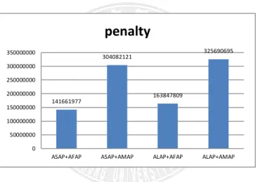
For soft-deadline jobs with the parallel-runtime charge model, the experimental results show that SJF is still the best waiting queue sequencing policy. However, in contrast to the scenario with the sequential-runtime charge model, AMAP is now a better spatial allocation policy than AFAP, as shown in Figures 5.6 and 5.7 that ASAP + AMAP achieves the largest profit. This implies that as the number of used processors increases the income grows more quickly than the penalty due to the degraded parallel efficiency for large numbers of processors reflected by the Amdahl’s Law [34].
Fig. 5.6 Penalty for soft-deadline jobs with parallel-runtime charge model and SJF policy
Fig. 5.7 Profit for soft-deadline jobs with parallel-runtime charge model and SJF policy
141661977 304082121 163847809 325690695 0 50000000 100000000 150000000 200000000 250000000 300000000 350000000
ASAP+AFAP ASAP+AMAP ALAP+AFAP ALAP+AMAP
penalty
3054510163 4186225149 2979564153 4116300199 0 500000000 1E+09 1.5E+09 2E+09 2.5E+09 3E+09 3.5E+09 4E+09 4.5E+09ASAP+AFAP ASAP+AMAP ALAP+AFAP ALAP+AMAP
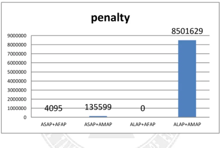
The following experiments deal with hard-deadline scenarios. Figures 5.8 to 5.12 are representative experimental results comparing the different combinations of temporal and spatial allocation policies of the reservation-based dynamic scheduling approach with the sequential-runtime charge model. For waiting queue sequencing, EDF was used in this scenario. The results show that ALAP + AFAP achieves the highest completion rate, allowing the most jobs to finish execution before deadline, and thus leads to the largest income. In addition, ALAP + AFAP results in the lowest deadline miss rate, i.e. zero percent as shown in Figure 5.8, and thus incurs the least penalty. Therefore, ALAP + AFAP achieves the largest profit among all methods.
Figures 5.13 and 5.14 is an illustrative example showing that why ALAP can achieve better performance than ASAP for hard-deadline scenarios. Table 5.1 shows the detailed attributes of the jobs in the example. In this example, ASAP leads to two more deadline misses, jobs 5.10 and 5.12. Comparing the resultant schedules in Figures 5.13 and 5.14, we can see that in ALAP jobs 6, 7, and 11 are reserved at later time periods, compared to in the ASAP schedule, leaving room for jobs 12 and 14, which arrive later, to meet their deadlines and thus accommodating more jobs for execution.
Fig. 5.8 Deadline miss rate for hard-deadline jobs with sequential-runtime charge model and the EDF policy
0.004% 0.147% 0.000% 2.305% 0.000% 0.500% 1.000% 1.500% 2.000% 2.500%
ASAP+AFAP ASAP+AMAP ALAP+AFAP ALAP+AMAP
Fig. 5.9 Completion rate for hard-deadline jobs with sequential-runtime charge model and the EDF policy
Fig. 5.10 Penalty for hard-deadline jobs with sequential-runtime charge model and the EDF policy
Fig. 5.11 Income for hard-deadline jobs with sequential-runtime charge model and the EDF policy
82.84% 70.43% 82.86% 75.44% 64.00% 66.00% 68.00% 70.00% 72.00% 74.00% 76.00% 78.00% 80.00% 82.00% 84.00%
ASAP+AFAP ASAP+AMAP ALAP+AFAP ALAP+AMAP
completion rate
4095 135599 0 8501629 0 1000000 2000000 3000000 4000000 5000000 6000000 7000000 8000000 9000000ASAP+AFAP ASAP+AMAP ALAP+AFAP ALAP+AMAP
penalty
468064582 444874510 468094136 444891020 430000000 435000000 440000000 445000000 450000000 455000000 460000000 465000000 470000000ASAP+AFAP ASAP+AMAP ALAP+AFAP ALAP+AMAP
Fig. 5.12 Profit for hard-deadline jobs with sequential-runtime charge model and the EDF policy
Fig. 5.13 An example with ALAP
Fig. 5.14 An example with ASAP
468060487 444738911 468094136 436389391 420000000 425000000 430000000 435000000 440000000 445000000 450000000 455000000 460000000 465000000 470000000 475000000
ASAP+AFAP ASAP+AMAP ALAP+AFAP ALAP+AMAP
Table 5.1 Job attributes and miss counts
ID Arrival Deadline Missed in ALAP Missed in ASAP 0 522378 539046 1 559483 727820 2 566290 616145 3 567314 577406 4 574294 607697 5 576100 580888 6 577685 899394 7 578846 620537 8 581034 590267 9 581434 585102 10 582841 599299 11 583532 619515 12 584801 591247 13 584826 584875 14 584832 585792 15 584875 584942
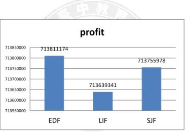
Figures 5.15 to 5.17 evaluate the waiting queue sequencing policies for hard-deadline scenarios with the sequential-runtime charge model. The experimental results show that EDF leads to the highest completion rate and the lowest penalty-attributed deadline-missed rate, resulting in the largest profit.
0.000% 0.005% 0.004% 0.000% 0.001% 0.002% 0.003% 0.004% 0.005% 0.006% EDF LIF SJF
deadline missrate
Fig. 5.15 Deadline miss rate for hard-deadline jobs with sequential-runtime charge model and ALAP+AFAP
policy
Fig. 5.16 Completion rate for hard-deadline jobs with sequential-runtime charge model and ALAP+AFAP policy
Fig. 5.17 Profit for hard-deadline jobs with sequential-runtime charge model and ALAP+AFAP policy
For scenarios with the parallel-runtime charge model, as shown in Figures 5.18 to 5.22, the ALAP + AMAP combination in general achieves the largest income among all temporal and spatial allocation methods although it leads to neither the highest completion rate nor the lowest deadline miss rate. As in the scenario of soft-deadline with the parallel-runtime charge model, this is because as the number of used processors increases the income grows more quickly than the penalty due to the degraded parallel efficiency for large numbers of processors reflected by the Amdahl’s Law [34]. The highest income of ALAP + AMAP leads it to the largest profit.
82.862% 82.852% 82.857% 82.846% 82.848% 82.850% 82.852% 82.854% 82.856% 82.858% 82.860% 82.862% 82.864% EDF LIF SJF
completion rate
713811174 713639341 713755978 713550000 713600000 713650000 713700000 713750000 713800000 713850000 EDF LIF SJFprofit
Fig. 5.18 Deadline miss rate for hard-deadline jobs with parallel-runtime charge model and the LIF policy
Fig. 5.19 Completion rate for hard-deadline jobs with parallel-runtime charge model and the LIF policy
Fig. 5.20 Penalty for hard-deadline jobs with parallel-runtime charge model and the LIF policy
0.007% 0.106% 0.005% 2.006% 0.000% 0.500% 1.000% 1.500% 2.000% 2.500%
ASAP+AFAP ASAP+AMAP ALAP+AFAP ALAP+AMAP
deadline missrate
82.82% 68.20% 82.85% 72.95% 0.00% 10.00% 20.00% 30.00% 40.00% 50.00% 60.00% 70.00% 80.00% 90.00%ASAP+AFAP ASAP+AMAP ALAP+AFAP ALAP+AMAP
completion rate
7393 115035 97413700 4407401 0 20000000 40000000 60000000 80000000 100000000 120000000ASAP+AFAP ASAP+AMAP ALAP+AFAP ALAP+AMAP
Fig. 5.21 Income for hard-deadline jobs with parallel-runtime charge model and the LIF policy
Fig. 5.22 Profit for hard-deadline jobs with parallel-runtime charge model and the LIF policy
For the waiting queue sequencing policies, the Largest Income First (LIF) policy is effective as shown in Figures 5.23 to 5.27. It leads to the largest income, shown in Figure 5.26, although with the lowest completion rate, shown in Figure 5.24. This implies that LIF can effectively maximize the income by favoring larger jobs. Since it also leads to the lowest deadline miss rate and thus the lowest penalty, shown in Figures 5.23 and 5.25, the LIF policy finally achieves the largest profit as shown in Figure 5.27.
713573846 2550157692 713643173 2583232192 0 500000000 1E+09 1.5E+09 2E+09 2.5E+09 3E+09
ASAP+AFAP ASAP+AMAP ALAP+AFAP ALAP+AMAP
Income
713566453 2550042657 713639341 2578824791 0 500000000 1E+09 1.5E+09 2E+09 2.5E+09 3E+09ASAP+AFAP ASAP+AMAP ALAP+AFAP ALAP+AMAP
Fig. 5.23 Deadline miss rate for hard-deadline jobs with parallel-runtime charge model and the ALAP+AMAP
policy
Fig. 5.24 Completion rate for hard-deadline jobs with parallel-runtime charge model and the ALAP+AMAP
policy
Fig. 5.25 Penalty for hard-deadline jobs with parallel-runtime charge model and the ALAP+AMAP policy
2.305% 2.006% 2.011% 1.850% 1.900% 1.950% 2.000% 2.050% 2.100% 2.150% 2.200% 2.250% 2.300% 2.350% EDF LIF SJF
deadline missrate
75.44% 72.95% 75.59% 71.50% 72.00% 72.50% 73.00% 73.50% 74.00% 74.50% 75.00% 75.50% 76.00% EDF LIF SJFcompletion rate
8501629 4407401 9415658 0 1000000 2000000 3000000 4000000 5000000 6000000 7000000 8000000 9000000 10000000 EDF LIF SJFpenalty
Fig. 5.26 Income for hard-deadline jobs with parallel-runtime charge model and the ALAP+AMAP policy
Fig. 5.27 Profit for hard-deadline jobs with parallel-runtime charge model and the ALAP+AMAP policy
The following experiments compare the proposed reservation-based dynamic scheduling approach with previous methods, including the Algorithm 3 in [35] and a dynamic version of the moldable EDF method in [27]. Since the two previous methods were developed for jobs of hard deadlines. The comparisons were conducted with two hard-deadline scenarios based on the sequential-runtime and parallel-runtime charge models, respectively. The experimental results for the sequential-runtime charge model in Figures 5.28 to 5.30 shows that our approach, AFAP+ALAP+EDF, achieves the lowest deadline-missed penalty and the highest income, thus
2571971304 2583232192 2563991776 2.55E+09 2.555E+09 2.56E+09 2.565E+09 2.57E+09 2.575E+09 2.58E+09 2.585E+09 EDF LIF SJF
Income
2563469675 2578824791 2554576118 2.54E+09 2.545E+09 2.55E+09 2.555E+09 2.56E+09 2.565E+09 2.57E+09 2.575E+09 2.58E+09 2.585E+09 EDF LIF SJFprofit
leading to the largest profit. Our approach achieves 7% and 20% increase in profit, compared to moldable EDF and Algorithm 3, respectively.
Fig. 5.28 Comparing different methods by penalty for hard-deadline jobs with the sequential-runtime charge
model
Fig. 5.29 Comparing different methods by income for hard-deadline jobs with the sequential-runtime charge
model 0 4095 97431332 0 20000000 40000000 60000000 80000000 100000000 120000000
AFAP+ALAP+EDF moldableEDF Algorithm3
penalty
468094136 468064582 468063550 468045000 468050000 468055000 468060000 468065000 468070000 468075000 468080000 468085000 468090000 468095000 468100000AFAP+ALAP+EDF moldableEDF Algorithm3
Fig. 5.30 Comparing different methods by profit for hard-deadline jobs with the sequential-runtime charge
model
For the parallel-runtime charge model, although our approach, AMAP+ALAP+LIF, incurs more deadline-missed penalties compared to moldable EDF, shown in Figure 5.31, it still achieves the largest profit as shown in Figure 5.33. This is because our approach brings a larger income than other methods. The increase in profit achieved by our approach is 72% and 85%, compared to moldable EDF and Algorithm 3, respectively.
Fig. 5.31 Comparing different methods by penalty for hard-deadline jobs with the parallel-runtime charge
model 468094136 468060487 370632218 0 50000000 100000000 150000000 200000000 250000000 300000000 350000000 400000000 450000000 500000000
AFAP+ALAP+EDF moldableEDF Algorithm3
profit
4407401 4095 97431332 0 20000000 40000000 60000000 80000000 100000000 120000000AMAP+ALAP+LIF moldableEDF Algorithm3
Fig. 5.32 Comparing different methods by income for hard-deadline jobs with the parallel-runtime charge
model
Fig. 5.33 Comparing different methods by profit for hard-deadline jobs with the parallel-runtime charge model
Figure 5.34 compares the scheduling overhead of the evaluated methods in terms of their execution time for scheduling the total 56490 jobs in the experiments. It’s clear that the Algorithm 3 in [35] has the least overhead since it doesn’t perform resource reservation for each job in the waiting queue. Our AMAP+ALAP+LIF approach for the parallel-runtime charge model has lower overhead than moldable EDF [27] and our another method for the sequential-runtime charge model because the AMAP policy tries the amount of free processors from the largest value, and thus could find the appropriate amount of processors to meet the deadline more quickly than the AFAP policy which tries from one processor. Our
2583232192 713638067 468063550 0 500000000 1E+09 1.5E+09 2E+09 2.5E+09 3E+09
AMAP+ALAP+LIF moldableEDF Algorithm3
Income
2578824791 713633972 370632218 0 500000000 1E+09 1.5E+09 2E+09 2.5E+09 3E+09AMAP+ALAP+LIF moldableEDF Algorithm3
AFAP+ALAP+EDF approach for the sequential-runtime charge model has the largest overhead since the ALAP policy, which tries from the latest time instant, might need to try more time instants than the ASAP policy before finding an appropriate one, although having the advantage of lower deadline-miss rate.
Fig. 5.34 Comparison of scheduling overhead of different methods
In the proposed reservation-based dynamic scheduling approach described in Algorithm 1, the scheduler will perform partial re-scheduling when a new job arrives. The effects of partial re-scheduling have pros and cons. It might cause some jobs which already have resource reservations for meeting their deadlines become missing deadlines. On the other hand, it also raises the probability that the new job can reserve appropriate resources to meet its deadline. In the following, we present a series of experiments, Figures 5.35 to 5.40, to evaluate the effectiveness of partial re-scheduling on job arrival for hard-deadline scenarios. In the figures, with commitment represents that no partial re-scheduling is performed, and without commitment indicates that partial re-scheduling is enabled. For the with commitment policy, once a job gets resource reservation to meet its deadline upon its submission, it is guaranteed that the reservation won’t be changed. Therefore, there won’t be deadline-missed penalties, as shown in Figures 5.35 and 5.38. This is its potential benefit.
959 1776 2102 836 0 500 1000 1500 2000 2500
AMAP+ALAP+LIF moldableEDF AFAP+ALAP+EDF Algorithm3
The experimental results show that in general the with commitment policy achieves larger profits as shown in Figures 5.37 and 5.40. However, the completion rate of the with commitment policy is lower than its counterpart for the sequential-runtime charge model, shown in Figure 5.36, while being higher than the without commitment policy for the parallel-runtime charge model, shown in Figure 5.39.
Fig. 5.35 Evaluation of deadline-miss rate for partial re-scheduling in hard-deadline scenarios with the
sequential-runtime charge model
Fig. 5.36 Evaluation of completion rate for partial re-scheduling in hard-deadline scenarios with the
sequential-runtime charge model 0.000% 0.002% 0.000% 0.001% 0.001% 0.002% 0.002% 0.003%
with commitment without commitment
deadline missrate
82.831% 82.832% 82.830% 82.831% 82.831% 82.831% 82.831% 82.831% 82.832% 82.832% 82.832% 82.832%with commitment without commitment
Fig. 5.37 Evaluation of profit for partial re-scheduling in hard-deadline scenarios with the sequential-runtime
charge model
Fig. 5.38 Evaluation of deadline-miss rate for partial re-scheduling in hard-deadline scenarios with the
parallel-runtime charge model
Fig. 5.39 Evaluation of completion rate for partial re-scheduling in hard-deadline scenarios with the
parallel-runtime charge model 464836393 464835664 464835200 464835400 464835600 464835800 464836000 464836200 464836400 464836600
with commitment without commitment
profit
0.000% 2.006% 0.000% 0.500% 1.000% 1.500% 2.000% 2.500%with commitment without commitment
deadline missrate
74.944% 72.953% 71.500% 72.000% 72.500% 73.000% 73.500% 74.000% 74.500% 75.000% 75.500%with commitment without commitment
Fig. 5.40 Evaluation of profit for partial re-scheduling in hard-deadline scenarios with the parallel-runtime charge model 2599593858 2578824791 2.565E+09 2.57E+09 2.575E+09 2.58E+09 2.585E+09 2.59E+09 2.595E+09 2.6E+09 2.605E+09
with commitment without commitment
Chapter 6. Conclusions
This thesis presents a reservation-based dynamic scheduling approach for deadline-constrained moldable jobs. The goal is to maximize the service provider’s profit. This is an emerging research topic as HPC as a Service [1] becomes a future trend for high performance computing, but not yet receives enough research attention.
The proposed approach is actually a scheduling framework involving three important scheduling and allocation issues, including waiting queue sequencing, temporal resource allocation, and spatial resource allocation. To deal with this emerging research topic, we first defined the profit model, charge model and penalty model to be used in performance evaluation. Then, we proposed several policies for the above three issues, including EDF, SJF, LIF for waiting queue sequencing; ASAP, ALAP for temporal resource allocation, and AFAP, AMAP for spatial resource allocation.
We conducted a series of simulation experiments to evaluate our reservation-based dynamic scheduling approach. The experimental results show that our approach can effectively increase the revenue of HPCaaS providers for both types of charge models, achieving 7% to 85% increase in different scenarios compared to moldable EDF [35] and the Algorithm 3 in [27]. However, the experimental results also indicate that careful selection of scheduling and allocation policies is essential since the best combination usually depends on the types of deadline and charge models. For example, for soft-deadline jobs, ASAP + AFAP + SJF is the best for the sequential-runtime charge model, while ASAP + AMAP + SJF achieves the largest profit for the parallel-runtime charge model. For jobs of hard deadline, AFAP + ALAP + EDF performs best for the sequential-runtime charge model, and AMAP + ALAP + LIF leads to the
largest revenue for the parallel-runtime charge model. As HPCaaS is an emerging model, the characteristics of jobs, penalty model, charge model, and profit model are all evolving. Therefore, there will be many new research issues on parallel job scheduling to explore in the future.
References
[1] M. AbdelBaky, M. Parashar, H. Kim, Jordan K.E.,V. Sachdeva, J. Sexton, H. Jamjoom, Z.Y. Shae, G. Pencheva, R. Tavakoli and M. F. Wheeler, “Enabling High Performance Computing as a Service”, Proc. IEEE Computer, Vol. 45, pp. 72-80. IEEE Press, Oct., 2012.
[2] Cloud computing,
http://www.infoworld.com/d/cloud-computing/what-cloud-computing-really-means-031,
June 2014.
[3] V. Leung, G. Sabin, and P. Sadayappan., “Parallel Job Scheduling Policies to Improve Fairness - A Case Study.” In: Proc. 6th Intern. Workshop on Scheduling and Resource Management for Parallel and Distributed Syst, 2010.
[4] V. Subramani, R. Kettimuthu, S. Srinivasan, J. Johnston, and P. Sadayappan, “Selective Buddy Allocation for Scheduling Parallel Jobs on Clusters,” Proc. IEEE Int’l Conf. Cluster Computing, pp. 107–116, Sept. 2002.
[5] G. Stiehr and R. D. Chamberlain., “Improving Cluster Utilization Through Intelligent.” In: Proceedings of 20th International Parallel and Distributed Processing Symposium, IPDPS, 2006.
[6] D. G. Feitelson, L. Rudolph, Schweigelshohn, U., Sevcik, K., and Wong. P. , “Theory and Practice in Parallel Job Scheduling. “, In: Job Scheduling Strategies for Parallel Processing, pp. 1-34, Springer-Verlag, Lecture Notes in Computer Science Vol. 1291, 1997.
[7] HPL benchmark, http://www.netlib.org/benchmark/hpl/ , June 2014.
[8] The Message Passing Interface standard, http://www.mcs.anl.gov/research/projects/mpi/ , June 2014.
[9] S. Baruah and J. Goossens., “The EDF Scheduling of Sporadic Task Systems on Uniform Multiprocessors.”, In: Proceedings of the 29th Real-Time Systems Symposium, 2008, pages 367–374, Dec. 2008.
[10] M. Bertogna, M. Cirinei, and G. Lipari., “Improved Schedulability Analysis of EDF on Multiprocessor Platforms.” In: Proceedings of the EuroMicro Conference on Real-Time
Systems, pages 209–218, Palma de Mallorca, Balearic Islands, Spain, IEEE Computer Society Press., July 2005.
[11] M. Bertogna, M. Cirinei, and G. Lipari., “New Schedulability Tests for Real-time Tasks Sets Scheduled by Deadline Monotonic on Multiprocessors.” In: Proceedings of the 9th International Conference on Principles of Distributed Systems, Pisa, Italy, IEEE
Computer Society Press, Dec. 2005.
[12] M. Cirinei and T. P. Baker., “EDZL scheduling analysis.” In Proceedings of the
EuroMicro Conference on Real-Time Systems, Pisa, Italy, IEEE Computer Society Press., July 2007.
[13] Parallel Workloads Archive, http://www.cs.huji.ac.il/labs/parallel/workload/ , June 2014. [14] S. Srinivasan, R. Kettimuthu, V. Subrarnani, and P. Sadayappan, “Characterization of
Backfilling Strategies for Parallel Job Scheduling”. In: Int’l Conf. on Parallel Processing (ICPP), pp. 514–522, Aug. 2002.
[15] A.K.L.Wong and A.M. Goscinski, "Evaluating the EASY- Backfill Job Scheduling of Static Workloads on Clusters," in Cluster Computing, 2007 IEEE International Conference, pp. 64-73., 2007.
[16] A. K. Wong and A. M. Goscinski, “The Impact of Under-estimated Length of Jobs on Easy-backfill Scheduling” In: Parallel, Distributed and Network-Based Processing IEEE, 2008.
[17] W. Cirne and F. Berman, “Using Moldability to Improve the Performance of Supercomputer Jobs”, Journal of Parallel and Distributed Computing, Vol. 62, pp. 1571-1601, Oct. 2002.
[18] K. C. Huang, “Performance Evaluation of Adaptive Processor Allocation Policies for Moldable Parallel Batch Jobs.” In: 3th Workshop on Grid Technologies and Applications, 2006.
[19] S. Srinivasan, S. Krishnamoorthy and P. Sadayappan, “A Robust Scheduling Strategy for Moldable Scheduling of Parallel Jobs.” In: 5th IEEE International Conference on
Cluster Computing, pp. 92-99, 2003.
[20] S. Srinivasan., V. Subramani, R. Kettimuthu, P. Holenarsipur and P. Sadayappan,
“Effective Selection of Partition Sizes for Moldable Scheduling of Parallel Jobs.” In: 9th International Conference on High Performance Computing, Springer, Lecture Notes In