計算結構生物學：在構形亂度和蛋白質動態上的研究

全文

(1)國立交通大學生物資訊所博士論文. 計算結構生物學：在構形亂度和蛋白質動態上的研究 Computational Structural Biology Studies on: I. Conformational entropy II. Protein dynamics . 研究生：黃少偉指導教授：黃鎮剛教授. 中華民國九十七年九月.

(2) 計算結構生物學：在構形亂度和蛋白質動態上的研究 Computational Structural Biology Studies on: I. Conformational entropy II. Protein dynamics. 研究生：黃少偉. Student：Shao-Wei Huang. 指導教授：黃鎮剛. Advisor：Jenn-Kang Hwang. 國立交通大學生物資訊所博士論文. A Dissertation Submitted to Institute of Bioinformatics College of Biological Science and Technology National Chiao Tung University in Partial Fulfillment of the Requirements for the Degree of PhD in Bioinformatics September 2008 Hsinchu, Taiwan, Republic of China. 中華民國九十七年九月.

(3) 計算結構生物學：在構形亂度和蛋白質動態上的研究. 學生：黃少偉. 指導教授：黃鎮剛. 國立交通大學生物資訊研究所博士班. 摘. 要. 一段蛋白質序列通常會構成一個獨特的立體結構，但前人的研究指出，不論是人工合成或是自然界存在的短序列片段，都發現到它們會在不同的結構環境中，形成不同的二級結構。這種短序列的特殊性質，最早是由 Kabsch 和 Sander 所發現的，在他們利用序列的相似性來預測蛋白質結構的研究中，發現了這個現象，並把有這類性質的短序列，命名為 chameleon (變色龍)。他們發現了許多長度為五個胺基酸的小序列片段，在不同的蛋白質裡面，形成了不同的二級結構。相反的，有些小序列片段，不管在什麼蛋白質中，都形成相同的二級結構，這樣子的序列片段，稱為有高度的結構保守性 (structure conservation)，而具 chameleon 性質的序列片段，其結構保守性則很低。在這部份的工作裡，我們利用 Support vector machine，開發了一種預測蛋白質短序列片段之結構保守性的方法。而我們將預測的結果，和 Hydrogen isotope exchange 實驗互相比較，發現了高度結構保守性的胺基酸，通常也具有緩慢的 Hydrogen isotope exchange 速率。研究蛋白質的動態 (dynamics)是分子生物學研究中，一個很重要. -- i.

(4) 的課題。最典型的計算生物學方法是分子動態模擬 (molecular dynamics simulation，MD)，這種方法計算原子和原子間的交互作用：鍵能、電荷作用等等。雖然 MD 的計算很精確，但是缺點是需要大量的計算時間和參數調整。另一種方法是 Gaussian network model (GNM)，它把蛋白質結構轉換成一個 Cα原子連結而成的網路結構， GNM 可以估算出個別胺基酸的熱擾動 (thermal fluctuation)以及胺基酸之間的動態相關性 (correlation of motion)。最近由本實驗室開發的方法 Protein-fixed-point (PFP). model，是一個非常簡單而準確的方. 法，所需要的資訊只有胺基酸 Cα原子的空間座標。首先決定整個蛋白質構造的重心 (center of mass)座標，我們發現某一胺基酸的熱擾動大小，和它到蛋白質重心的距離平方成正比例的關係。另一個本實驗室開發的方法是 Weighted-contact number (WCN) model，它計算胺基酸周圍的原子數目，愈接近的原子可以得到較高的權重 (weight)，反之則影響較小。胺基酸若處於有很多原子集結的環境，則熱擾動的值較小。PFP 和 WCN model 的結果顯示，蛋白質的動態資訊，可以單純的由它的結構推算出來，並不需要做任何機械模型的假設 (如 GNM)。在這部份的研究，為了驗證 PFP 和 WCN model 的正確性，我們利用這兩個方法來預測蛋白質的 NMR order parameter，並和實驗值相比較。這兩種方法的預測結果都比前人所做的方法要好。蛋白質的功能通常會牽涉到結構上大規模的運動 (large scale motion)。Normal mode analysis (NMA)早在 1980 年開始，就被用來研究蛋白質的大規模運動，它最主要的特點是把蛋白質的動態拆解成很多不同頻率的運動，包含了頻率較低、較大規模的運動，以及頻率較高、較小規模的運動。生物學家通常感興趣的部份是頻率較低、較大規模的運動，因為通常這類的運動和蛋白質的功能表現有最直接的關. -- ii.

(5) 係。NMA 最早是把 MD 模擬當中的位能函數 (potential function)做二次微分得到 Hessian matrix，再對它做對角化 (diagonalize)運算後，得到蛋白質中各種不同頻率的運動。而這個方法的缺點是，在計算較大的蛋白質時，計算時間會變的非常龐大。另一種方法是 Elastic network model (ENM)，它把蛋白質結構轉換成一個 Cα原子連結而成的網路結構，基於這個網路結構，前人開發出了一種簡化版本的 NMA，它大幅減小了所需要的計算時間，並且也可以得到非常好的結果。現今最廣泛被使用的 ENM 方法是 Gaussian network model (GNM)。本實驗室所研發的 PFP model，是一種簡單，同時可以準確預測胺基酸熱擾動的方法，我們基於 PFP model，研發出了另一種 NMA 的方法，在這部份的研究裡，我們將 PFP model 的 NMA 結果，和 GNM 的結果相比較，並且發現了它們在所研究的例子裡，大致上有相吻合的結果。. -- iii.

(6) Computational Structural Biology Studies on: I. Conformational entropy II. Protein dynamics student：Shao-Wei Huang. Advisors：Dr.Jenn-Kang Hwang. Institute of Bioinformatics National Chiao Tung University. ABSTRACT. A complete protein sequence usually determines a unique structure; however the situation is different for shorter subsequence. Studies found that both designed and nature occurring subsequences may have different secondary structures in different contexts. This feature of short sequence is called “chameleon” which was first reported by Kabsch and Sander when they used sequence homology to predict protein structures. They found that several pentapeptides which have identical sequence adopt different secondary structures in different protein structures. For nature occurring proteins, systematic search on PDB shows that identical subsequences could have very different conformations. Here we developed a method to compute structure conservation from protein sequence. During protein folding process, there are some structured regions which are similar to folded conformation. Hydrogen isotope exchange (HX) rate is usually used to identify those structured regions. We applied this method to a set of proteins with known HX rate data and found a strong correlation between structure conservation and slow HX -- iv.

(7) rate. One of the most important topics in biological science is to understand the protein function. It is well-known that protein dynamics is closely related to the function of protein. Several computational methods have been developed to get the protein dynamics. Molecular dynamics (MD) simulation has been widely used in the study of protein function and dynamics. It simulates the interactions between each atom, bonding force, van der Waals force, charge-charge interaction, etc. The computation time is extremely long when the size of the protein is large and the selection of appropriate parameters of force field itself is a complicated problem. Gaussian network model (GNM) transfers the protein structure into a network in which each Cα atom pair is connected together if their distance is smaller than a given cutoff value. Using this protein-converted network, GNM can compute the theoretical thermal fluctuation of each atom and correlation of motions between each atom pair. Recently we have developed a model to predict the thermal fluctuation from protein structure, which is called protein-fixed-point (PFP) model. The PFP model only uses the coordinates of Cα atoms and simply determines the center of mass of the protein. We found that the thermal fluctuation is proportional to the squared distance from the atom to the center of mass of the structure. Another model called weighted contact number (WCN) model computes the number of neighboring atoms weighted by the inverse distance between each atom pair. The PFP and WCN model show that the protein dynamics can be extracted directly from the intrinsic property of protein structure without the use of any mechanical model. The order parameter obtained by the NMR experiment is widely used to study the dynamic-related protein functions. Here, we use the PFP and WCN model to predict the N-H S2 order parameter directly from the protein structure. Our results show that the WCN model -- v.

(8) can more accurately reproduce the experimental order parameter than previous publication. The biological function of proteins is closely related to cooperative motions and correlated fluctuations which involve large portions of the structure.. Normal Mode Analysis (NMA) had been used to study. biomolecules since early 1980s. It decomposes the protein dynamics into a collection of motions which include large scale/low frequency and small scale/high frequency motions. Biologists usually focus on the large scale/low frequency motions which are relevant to protein functions. The major contribution of NMA to the biological research field is the ability to provide the information of large, domain-scale protein motions which is hard to compute by other methods. The classical approach of NMA is to diagonalize the Hessian matrix, i.e. the second derivative of the potential function of a molecular dynamics (MD) simulation. The major shortcoming of the classical NMA is that the sampling time increases dramatically with the size of the protein. The Elastic Network Model (ENM), which is able to describes protein dynamics without amino acid sequence and atomic coordinates, has been widely used in the studies of protein dynamics and structure-function relationship. The ENM views the protein structure as an elastic network, the nodes of which are the Cα atoms of individual residues. Residue pairs within a cutoff distance are connected by springs which have a uniform force constant in the network. Based on ENM, a coarse-grained version of NMA is developed and widely used because of its low computation cost and the ability to extend the dynamics to longer timescale and larger motions. The coarse-grained NMA had been applied to various topics, for example, protein functions and catalytic residues. One of the most widely used ENM-based methods is the Gaussian network model (GNM). The protein-fixed-point (PFP) -- vi.

(9) model is a simple method to compute the protein dynamics only using the coordinates of Cα atoms. Despite its simplicity, it has been shown to be able to accurately predict the B-factors for a dataset of 972 proteins. Here, we compared the results of NMA based on the PFP model with those by Gaussian network model (GNM).. -- vii.

(10) 誌謝. 感謝我的指導教授黃鎮剛老師，從我大學三年級做專題開始，一直到現在七年來的耐心教導，啟發了我對生物資訊方面研究的興趣和熱忱。感謝大學的班導師彭慧玲老師，從大學到研究所一直關心班上同學的生活和發展，給我們很多鼓勵和各方面的幫助。謝謝楊進木老師、黃憲達老師、呂平江老師、林彩雲老師在學位考試的指導和對論文需要改進地方的建議，讓我了解到自己不足和需要加強的地方。感謝玉菁學姐、春吟學姐在我做專題生時熱心的幫忙。大熊學長、勇欣學長、景盛學長、禎祥學長、涵堃學長對於研究方面的幫助。最照顧學弟妹的草霸、志鵬、鐵雄、志杰學長們，有好康的東西總不會忘記我們。碩班同時進實驗室的戰友，小操、建華、啟德、肇基、蔚倫，和你們一起修課、努力做研究的日子是最難忘的。感謝實驗室的學弟妹們：世瑜、思樸、書瑋、彥龍、小胖、啟文、阿壁、松桓、仙蕾、慧雯、子琳、小芬、人維、乃文，為我們這些老人家帶來許多歡樂。讀研究所期間，感謝我的好朋友們在開心的時候一起分享歡樂、難過的時候互相陪伴，最會關心別人的健誠，常常陪我丟棒球的小操，沒事會招待我們去家裡玩的祐俊和怡伶夫婦；最會替別人著想的宗凰、彥均、庭毓，僑牌高手 Vic 和小新、常常開車帶我們出去玩的明宏，老羅學長、昱佑、劭恆、小宏，感謝你們的陪伴。特別感謝子慧四年來容忍我難相處的個性，給我無止盡的包容和鼓勵。最重要的感謝我的家人，爸爸和媽媽從小到大的照顧和關心，讓 --viii.

(11) 我能夠專心學習並且追求自己的興趣，在決定要攻讀博士學位的時候，也一直給我支持和鼓勵。能夠專注在一件事情上，並且堅持完成的態度，都是從你們身上學習到的，感謝你們!. -- ix.

(12) Index 中文摘要英文摘要誌謝 Index Tables Figures Abbreviations Chapter 1 1.1 1.2 1.3 1.4 Chapter 2 2.1 2.2 2.3 2.4 Chapter 3 3.1 3.2 3.3 3.4 Appendix A B C D E References. ……………………………………………………………… ……………………………………………………………… ……………………………………………………………… ……………………………………………………………… ……………………………………………………………… ……………………………………………………………… ……………………………………………………………… Computation of Conformational Entropy from Protein Sequence Introduction…………………………………………………. Methods…………………………………………………….. Results………………………………………………………. Discussion…………………………………………………... NMR Order Parameter Prediction Using Protein-fixed-point Model and Weighted Contact Number Model Introduction ………………………………………………… Methods ……………………………………………………. Results ……………………………………………………… Discussion ………………………………………………….. Normal Mode Analysis by the Protein-fixed-point Model Introduction ………………………………………………… Methods ……………………………………………………. Results……………………………………………………… Discussion…………………………………………………... i iv viii x xi xii xiv. ……………………………………………………………… ……………………………………………………………… ……………………………………………………………… ……………………………………………………………… ……………………………………………………………… ………………………………………………………………. 67 68 69 71 72 77. . -- x. 1 4 10 28. 30 34 36 47 49 51 53 64.

(13) Tables . Table 1 Table 2 Table 3 Table 4 Table 5. The predicted backbone N-H order parameters computed with the WCN, PFP, CM, and rCENM……………………... The Pearson correlation coefficient between the correlation maps computed by the PFP model and the GNM…………... RS126 dataset…………………….………………………… Hydrogen exchange dataset………………………………… Normal mode analysis dataset………………………………. -- xi. 36 53 67 68 71.

(14) Figures Figure 1 Figure 2 Figure 3 Figure 4 Figure 5 Figure 6 Figure 7 Figure 8 Figure 9 Figure 10 Figure 11 Figure 12 Figure 13 Figure 14 Figure 15 Figure 16 Figure 17 Figure 18 Figure 19 Figure 20 Figure 21 Figure 22 Figure 23. The AVLAE sequence (red color) forms an α-helix in potassium channel (right, 1BL8) but forms a β-sheet in a transposase inhibitor (left, 1B7E)……………………………………………………………. Flowchart of conformational entropy calculation from protein sequence………………………………………………………………. Maximum-margin hyperplanes for a SVM trained with samples from two classes. Samples along the hyperplanes are called the support vectors…………………………………………………………………. Conformational entropy profile of hen egg-white lysozyme………….. Spatial distribution of residues with the slowest exchanging protons (blue) and the lowest conformational entropy (red) on the ribbon diagram of hen egg-white lysozyme…………………………………... Conformational entropy profile of chymotrypsin inhibitor 2…………. Spatial distribution of residues with the slowest exchanging protons (blue) and the lowest conformational entropy (red) on the ribbon diagram of chymotrypsin inhibitor 2………………………………….. Conformational entropy profile of cytochrome c……………………... Spatial distribution of residues with the slowest exchanging protons (blue) and the lowest conformational entropy (red) on the ribbon diagram of cytochrome c……………………………………………… Conformational entropy profile of each unfolding unit of cytochrome c and the corresponding average values………………………………. Conformational entropy profile of barnase……………………………. Spatial distribution of residues with the slowest exchanging protons (blue) and the lowest conformational entropy (red) on the ribbon diagram of barnase…………………………………………………….. Conformational entropy profile of α-lactalbumin……………………... Spatial distribution of residues with the slowest exchanging protons (blue) and the lowest conformational entropy (red) on the ribbon diagram of α-lactalbumin……………………………………………… Conformational entropy profile of CTX III…………………………… Spatial distribution of residues with the slowest exchanging protons (blue) and the lowest conformational entropy (red) on the ribbon diagram of CTX III……………………………………………………. Conformational entropy profile of ribonuclease H …………………… Spatial distribution of residues with the slowest exchanging protons (blue) and the lowest conformational entropy (red) on the ribbon diagram of ribonuclease H…………………………………………….. Conformational entropy profile of BPTI……………………………… Spatial distribution of residues with the slowest exchanging protons (blue) and the lowest conformational entropy (red) on the ribbon diagram of BPTI………………………………………………………. Superposition of apo Aquifex Adk (red) and Aquifex Adk in complex (green)…………………………………………………………………. Predicted and experimental order parameter of βARK1 PH domain…. Predicted and experimental order parameter of Calbindin……………. -- xii. 2 4 5 10 11 12 13 14 15 16 18 19 20 21 22 23 24 25 26 27 30 37 38.

(15) Figure 24 Figure 25 Figure 26 Figure 27 Figure 28 Figure 29 Figure 30 Figure 31 Figure 32 Figure 33 Figure 34 Figure 35 Figure 36 Figure 37 Figure 38 Figure 39 Figure 40. Predicted and experimental order parameter of Cold-shock protein A from E-coli…………………………………………………………….. Predicted and experimental order parameter of Frenolicin acyl carrier protein…………………………………………………………………. Predicted and experimental order parameter of Lysozyme…………… Predicted and experimental order parameter of SH2 domain of p85 subunit of phosphoinositide 3-kinase………………………………….. Predicted and experimental order parameter of Ubiquitin…………….. Predicted and experimental order parameter of Ketosteroid isomerase. Predicted and experimental order parameter of 4-oxalocrotonate Tautomerase…………………………………………………………… Predicted and experimental order parameter of Interleukin-4………… The correlation maps of (a) Prot-glu methylesterase (1RPT), (b) Ribonuclease T2 (1BOL), and (c) Uridine nucleosidase (1EUG) computed with the PFP model (left) and GNM (right), respectively…. Distribution of displacements along the first mode, second mode, and third mode computed for thiol-endopeptidase (9PAP)........................... The regions subject to opposite direction displacements computed by the PFP model (left) and the GNM (right) of (a) the first mode, (b) the second mode, and (c) the third mode for thiol-endopeptidase (9PAP)... Ribbon diagram colored blue-yellow-red in the order of increasing mobility along the first mode of the PFP model (left) and GNM (right)………………………………………………………………….. Distribution of displacements along the first mode, second mode, and third mode computed for G/11 xylanase (1BVV)................................... The regions subject to opposite direction displacements computed by the PFP model (left) and the GNM (right) of (a) the first mode, (b) the second mode, and (c) the third mode for G/11 xylanase (1BVV).......... The displacements of actinidin (1AEC) subject to opposite directions along the fist mode…………………………………………………….. Ribbon diagram of actinidin colored blue-yellow-red in the order of increasing mobility along the first mode……………………………... The flowchart of computing normal mode motions by PFP model and GNM………………………………………………………………….... --xiii. 39 40 41 42 43 44 45 46 54 57 58 59 60 61 62 63 65.

(16) Abbreviations Chapter 1 BLAST . Basic local alignment search tool . BPTI CI2 HEWL HX PSI‐BLAST PSSM . Bovine pancreatic trypsin inhibitor Chymotrypsin inhibitor 2 Hen egg‐white lysozyme Hydrogen exchange Position‐specific iterative BLAST Position‐specific substitution matrix . RNaseH SVM Chapter 2 . Ribonuclease H Support vector machine . CM CspA Frendicin ACP GNM MD PFP rCENM WCN Chapter 3 . Contact model Cold‐shock protein A Frendicin acyl carrier protein Gaussian network model Molecular dynamics Protein‐fixed‐point Reorientational contact‐weighted elastic network model Weighted contact number . ENM GNM MD NMA PFP . Elastic network model Gaussian network model Molecular dynamics Normal mode analysis Protein‐fixed‐point . . . . --xiv.

(17) CHAPTER ONE . Computation of Conformational Entropy from Protein Sequence . Introduction A complete protein sequence usually determines a unique structure; however the situation is different for shorter subsequence. Studies1‐4 on both designed and nature occurring subsequences found that they may have different secondary structures in different contexts. This feature of short sequence is called “chameleon“ which was first reported by Kabsch and Sander1 using sequence homology to predict protein structures. They found that several pentapeptides which have identical sequence adopt different secondary structures in different protein structures. For nature occurring proteins, systematic search1,3,4 on PDB5 shows that identical subsequences could have very different conformations. For example, the pentapeptide AVLAE forms an α‐helix in a potassium channel but forms a β‐sheet in a transposase inhibitor (Figure 1.1). Following the observation of Kabsch and Sander1, Cohen et al.6 discovered eight pairs of hexapeptides sequences which adopt α‐helix in one protein and β‐strand in the other using a larger protein dataset. .

(18) Figure 1.1 The AVLAE sequence (red color) forms an α‐helix in potassium channel (right, 1BL8) but forms a β‐sheet in a transposase inhibitor (left, 1B7E). . In additional to the studies focused on subsequences forming different secondary structures in different proteins, Minor and Kim2 artificially put a short sequence into different locations of a single protein. They designed an 11‐peptide sequence which folds as an α‐helix in one context while a β‐sheet in another. The designed subsequence (AWTVEKAFKTF) was replaced at different positions of IgG‐binding domain of protein G (GB1), and the subsequence was determined experimentally to fold into different conformations. However, some of the shorter subsequences are able to form unique conformation in different contexts. In the case of subsequence AALAE, the conformation remains the same α‐helix in different proteins. This property of structural conservation or variability is determined by the local and non‐local interactions. . 2.

(19) Here we developed a method to compute structure conservation from protein sequence. The main idea is to predict, for each residue, the possibilities distribution of each secondary structure type. Based on the distribution, a conformational entropy value is computed for each residue and is assumed to be related to the structural conservation. The low conformational entropy parts indicate highly structural conserved regions. During protein folding process, there are some structured regions which is similar to folded conformation7‐10. Hydrogen isotope exchange (HX) rate11‐13 is usually used to identify those structured regions. We applied this method to a set of proteins with known HX rate data and found a strong correlation between structure conservation and slow HX rate. . 3.

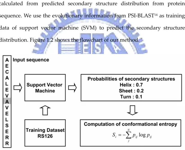
(20) . Methods . Overview The structure conservation (conformational entropy) of each residue is calculated from predicted secondary structure distribution from protein sequence. We use the evolutionary information from PSI‐BLAST14 as training data of support vector machine (SVM) to predict the secondary structure distribution. Figure 1.2 shows the flowchart of our method. . Figure 1.2 Flowchart of conformational entropy calculation from protein sequence. . 4.

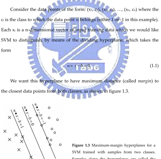
(21) The Support Vector Machine The idea of support vector machine method (SVM)15 is to find the separating hyperplane with largest distance between two classes. However in many cases, the data can not be separated linearly. To solve this problem, SVM uses kernel functions to nonlinearly transform the input space into higher dimensional feature space, and the data may be well separated in the higher dimensional space. Consider the data points of the form: (x1, c1), (x2, c2), …, (xn, cn) where the ci is the class to which the data point xi belongs (either 1 or ‐1 in this example). Each xi is a n‐dimensional vector of input training data which we would like SVM to distinguish, by means of the dividing hyperplane, which takes the form w × x − b = 0 (1.1) We want this hyperplane to have maximum distance (called margin) to the closest data points from both classes, as shown in figure 1.3. . Figure 1.3 Maximum‐margin hyperplanes for a SVM trained with samples from two classes. Samples along the hyperplanes are called the support vectors. . 5.

(22) The maximum‐margin hyperplane can be defined by finding the parallel hyperplanes closest to the support vectors in either class. These parallel hyperplanes can be described by equations w× x − b = 1 (1.2) w × x − b = −1. We would like these hyperplanes to have maximum distance from the dividing hyperplane and no data points between them. To exclude data points, all i must satisfy either w × xi − b ≥ 1 (1.3) or w × x i −b ≤ −1 (1.4) We can rewrite this to ci ( w × xi − b) ≥ 1 1≤ i ≤ n. . . . (1.5) . So we want to maximize the distance between the hyperplanes (2/|w|) subject to the constraint (1.5). After training, we can use SVM to classify test data points by following decision rule ⎧ 1, if w × x + b ≥ 0 cˆ = ⎨ (1.6) ⎩− 1, if w × x + b ≤ 0 SVM had been successfully applied to secondary structure prediction16‐18, solvent . accessibility . prediction19, . fold . assignment20,21, . subcellular . localization22,23 and other computation biology problems24‐26. In this work, the . 6.

(23) software package LIBSVM27 was used. . Computation of Conformational Entropy The conformational entropy of each residue is calculated from predicted secondary structure distribution from protein sequence. We use the evolutionary information from PSI‐BLAST14 as training data of SVM to predict the secondary structure distribution. PSI‐BLAST BLAST (Basic local alignment search tool) is used to search similar sequences of a query sequence from a large database. The algorithm will find subsequences of the query resemble to the subsequences of database. PSI‐BLAST (Position‐specific iterative BLAST) is developed to find distant homologues. After the first round of BLAST search, sequences which are similar to the query sequence are collected and combined into a profile. This profile is called position‐specific substitution matrix (PSSM) and is used as query in the second round of search against the database. The rebuilding of profile and searching procedure is then repeated. PSSM contains the information of relate sequences and is more sensitive in finding distant relate sequences. Secondary structure definition In this work, the secondary structure is defined by DSSP28 program. DSSP assigns secondary structures of a given 3D structure according to the atom coordinates and hydrogen bonding patterns. Eight classes of secondary 7.

(24) structures are defined in DSSP • •. H = α‐helix B = residue in isolated β‐bridge . •. E = extended strand, participates in β ladder . •. G = 3/10 helix I = π‐helix . • • • •. T = hydrogen bonded turn S = bend U = undefined . Conformational entropy calculation We compute the probability distribution of the secondary structure by SVM. The inputs of SVM are in the form of W * 20 PSSM profiles, where W is the sliding window size. The sliding window is used to include the information of neighboring residues on sequence. In the work, window size is chosen to be 15. PSSM profile is obtained after 3 iterations of PSI‐BLAST search against a non‐redundant database with the E‐value threshold set to 1 * 10‐3. Each element in PSSM profile represents the score of a particular residue substitution at that position. These elements are usually in the range ± 7 and are normalized to the range [0, 1] by the following function if x ≤ - 5 ⎧ 0.0 ⎪ π ( x) = ⎨0.5 + 0.1x if - 5 ≤ x ≤ 5 ⎪ 1.0 if x ≥ 5 ⎩. 8. . . (1.7) .

(25) where x is the original matrix element value. The output of SVM for the target residue is an eight‐element vector O = (o1, o2, …,o8), where oi is the decision value of secondary structure type i. The output of SVM does not give the probability for each classification, so we use a function [arctan(oi)+π] to transform the decision value to probability in the range [0, 1]. With P=(p1, p2, …, p8), where pi is the probability of secondary type i of target residue, we calculate conformational entropy by the following equation N. S i = −∑ p ij log pij (1.8) j. where Si is the conformational entropy of residue i, and pij is the probability of residue i classified to be secondary type j. N is the number of secondary structure types. . Training Dataset We train SVM using a standard non‐redundant dataset RS12629, with sequence identity less than 25% over a length of more than 80 residues. See appendix A for more detail. . 9.

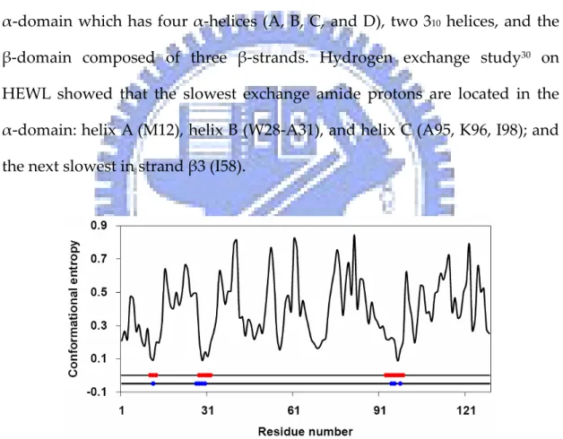
(26) . Results . Hen egg‐white lysozyme . Hen egg‐white lysozyme (HEWL) contains two sub‐domains: the . α‐domain which has four α‐helices (A, B, C, and D), two 310 helices, and the β‐domain composed of three β‐strands. Hydrogen exchange study30 on HEWL showed that the slowest exchange amide protons are located in the α‐domain: helix A (M12), helix B (W28‐A31), and helix C (A95, K96, I98); and the next slowest in strand β3 (I58). . Figure 1.4 Conformational entropy profile of hen egg‐white lysozyme. Residues with the slowest exchanging protons (blue) and the lowest conformational entropy (red) are labeled. . 10.

(27) Figure 1.4 shows the conformational entropy profile of HEWL. The lowest entropy regions are A11‐K13 (helix A), W28‐K33 (helix B), and N93‐V99 (helix C), respectively. These amino acids overlap with the slow exchange amide protons in helices A, B, and C. Note the residues in helix D (V109‐R114) have relatively higher entropy. This result is supported by the experiment that amino acids in helix D have much higher amide exchange rate. Figure 1.5 is the ribbon diagrams of HEWL colored by low conformational entropy and slow exchange regions. . Figure 1.5 Spatial distribution of residues with the slowest exchanging protons (blue) and the lowest conformational entropy (red) on the ribbon diagram of hen egg‐white lysozyme. . . 11.

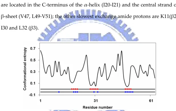
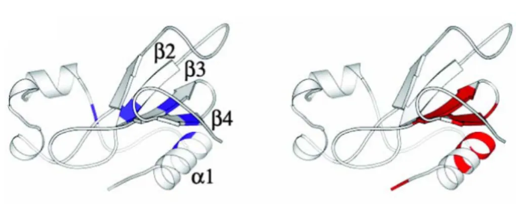
(28) Chymotrypsin inhibitor 2 Chymotrypsin inhibitor 2 (CI2) is a monomeric protein of 64 residues and folds by simple two‐state kinetics. The only well developed region during intermediate state is an N‐terminal α‐helix and some distant residues in sequence which contact with it. The α‐helix packs with the β‐sheet to form the hydrophobic core. Studies31,32 showed that the slowest exchange‐rate residues are located in the C‐terminus of the α‐helix (I20‐I21) and the central strand of β‐sheet (V47, L49‐V51); the other slowest exchange amide protons are K11(β2), I30 and L32 (β3). . Figure 1.6 Conformational entropy profile of chymotrypsin inhibitor 2. Residues with the slowest exchanging protons (blue) and the lowest conformational entropy (red) are labeled. . Figure 1.6 shows that most residues having the lowest conformational entropy overlap with those of the slowest hydrogen exchange rates, except K11. Most of them are on the α‐helix, β‐strands 3 and 4. Figure 1.7 compares the spatial distribution of the lowest conformational entropy and the slowest exchange‐rate regions on ribbon diagram of CI2. . 12.

(29) Figure 1.7 Spatial distribution of residues with the slowest exchanging protons (blue) and the lowest conformational entropy (red) on the ribbon diagram of chymotrypsin inhibitor 2.. 13.

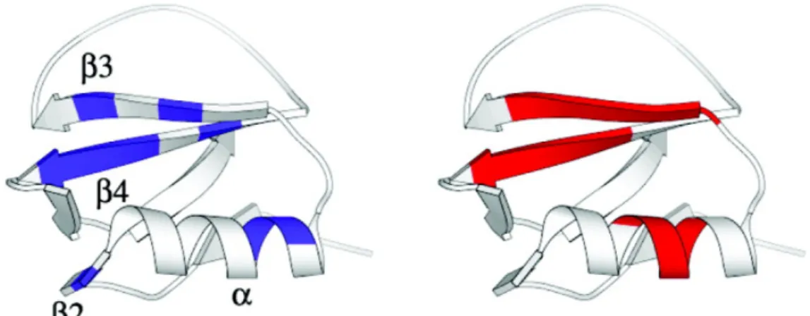
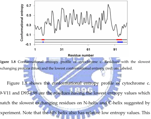
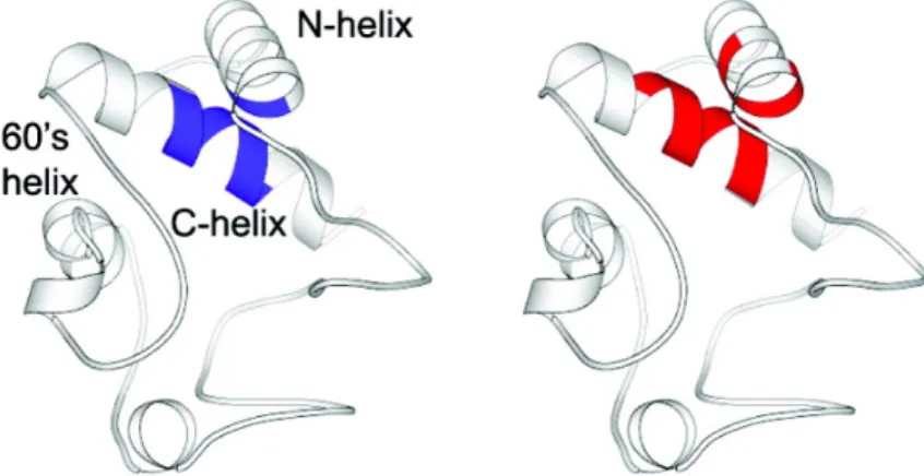
(30) Cytochrome c . Hydrogen exchange study33 shows that the slowest exchanging amide . protons are located in the three major helical segments of cytochrome c. F10 (N‐helix) and L94‐K99 (C‐helix) carry the slowest exchanging amide protons. . Figure 1.8 Conformational entropy profile of cytochrome c. Residues with the slowest exchanging protons (blue) and the lowest conformational entropy (red) are labeled. . . Figure 1.8 shows the conformational entropy profile of cytochrome c. . I9‐V11 and D93‐L98 are the residues having the lowest entropy values which match the slowest exchanging residues on N‐helix and C‐helix suggested by experiment. Note that the 60’s helix also has relative low entropy values. This is consistent with the experimental results that the next slowest exchanging amide protons are located in the 60’s helix. Figure 1.9 shows the spatial distribution of residues with the slowest exchanging protons and the lowest conformational entropy on ribbon diagram of cytochrome c. . 14.

(31) Figure 1.9 Spatial distribution of residues with the slowest exchanging protons (blue) and the lowest conformational entropy (red) on the ribbon diagram of cytochrome c. . . 15.

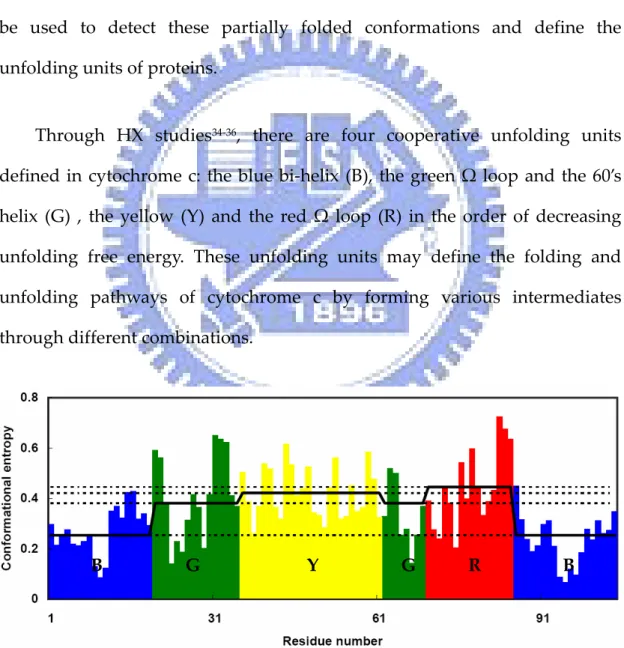
(32) Equilibrium Protein Folding . Cytochrome c is a good model system in studies34‐36 of protein folding . and unfolding. Under native conditions, most proteins exist in their unique native conformation. However some of them also exist in higher energy states and continue to cycle through totally unfolded states and partially folded states. These non‐native forms are usually hard to be detected because of the abundant native conformational signals. Hydrogen exchange experiment can be used to detect these partially folded conformations and define the unfolding units of proteins. . Through HX studies34‐36, there are four cooperative unfolding units . defined in cytochrome c: the blue bi‐helix (B), the green Ω loop and the 60’s helix (G) , the yellow (Y) and the red Ω loop (R) in the order of decreasing unfolding free energy. These unfolding units may define the folding and unfolding pathways of cytochrome c by forming various intermediates through different combinations. . B . G . Y. G. R. B . Figure 1.10 Conformational entropy profile of each unfolding unit of cytochrome c and the corresponding average values. . 16.

(33) . Figure 1.10 shows the conformational entropy profile of each unfolding . unit and the corresponding average values. Unit B has the lowest average conformational entropy, unit G has second lowest entropy, and then Y, and R. The order of increasing conformational entropy follows the order of decreasing unfolding free energy. . 17.

(34) Barnase Barnase has three α‐helices and a five‐stranded β‐sheet. The first helix packs onto the β‐sheet to form the major hydrophobic core of the protein. The second and the third α‐helices pack onto another side of the β‐sheet to form a smaller hydrophobic core. . Figure 1.11 Conformational entropy profile of barnase. Residues with the slowest exchanging protons (blue) and the lowest conformational entropy (red) are labeled. . Figure 1.11 shows the conformational entropy profile of barnase. Previous study37,38 showed that L14, I25, A74, L89 and Y97 have the lowest exchange rates. L14 on the first α‐helix and I25, A74 ad L89 on the β‐sheet are located in the major hydrophobic core of the protein. Y97 is in the center of the smaller hydrophobic core formed by the two smaller helices and part of the β‐sheet. Figure 1.12 shows the spatial distribution of residues with the slowest exchanging protons and the lowest conformational entropy on the ribbon diagram of barnase. . 18.

(35) Figure 1.12 Spatial distribution of residues with the slowest exchanging protons (blue) and the lowest conformational entropy (red) on the ribbon diagram of barnase.. 19.

(36) α‐Lactalbumin α‐lactalbumin is a calcium‐binding protein which consists of a β‐sheet domain and a α‐helical domain. The helical domain is composed of four helices: helix A (C6‐E11), helix B (P24‐S34), helix C (D87‐D97) and helix D (D102‐ L105). Previous studies39,40 showed that in the helical domain, the C‐helix is the most protected, having the lowest exchanging rate, followed by the B and then the A‐helix. . Figure 1.13 Conformational entropy profile of α‐lactalbumin. Residues with the slowest exchanging protons (blue) and the lowest conformational entropy (red) are labeled. . Figure 1.13 shows the profile of the conformational entropy. The residues in C‐helix have the lowest conformational entropy and the residues which have second lowest conformational entropy are located in helix B and helix A. The regions which have low conformational entropy are consistent with those having slow exchanging rate39,40. Note that a previous study40 showed that helix D exchanges too fast and the exchanging rates are not measurable. Our calculation also indicates that helix D has high conformational entropy. Figure 1.14 shows the spatial distribution of residues with the slowest exchanging . 20.

(37) protons and the lowest conformational entropy on the ribbon diagram of α‐lactalbumin. . Figure 1.14 Spatial distribution of residues with the slowest exchanging protons (blue) and the lowest conformational entropy (red) on the ribbon diagram of α‐lactalbumin.. 21.

(38) Cardiotoxin III Cardiotoxin III (CTX III) is a 60‐amino acid, all β‐sheet protein. The secondary structure of CTX III includes five β‐strands forming double and triple‐stranded anti‐parallel β‐sheets. Hydrogen exchange study41 on CTX III showed that residues K23, I39, and Y51‐N55 constitute the hydrophobic cluster of the protein. . Figure 1.15 Conformational entropy profile of CTX III. Residues with the slowest exchanging protons (blue) and the lowest conformational entropy (red) are labeled. . Figure 1.15 shows the conformational entropy profile of CTX III. Our calculation of low conformational entropy residues covers most of the slow exchange residues (Y22‐M24, V52). Figure 1.16 shows the spatial distribution of residues with the slowest exchanging protons and the lowest conformational entropy on the ribbon diagram of cardiotoxin III. . 22.

(39) Figure 1.16 Spatial distribution of residues with the slowest exchanging protons (blue) and the lowest conformational entropy (red) on the ribbon diagram of CTX III.. 23.

(40) Ribonuclease H Ribonuclease H (RNaseH) is a 155‐residue protein with four α‐helices packing with a five‐stranded β‐sheet. A previous study42 showed that helix A (T43‐L56) and helix D (V101‐L111) are the most stable regions in the protein. . . Figure 1.17 Conformational entropy profile of ribonuclease H. Residues with the slowest exchanging protons (blue) and the lowest conformational entropy (red) are labeled. . Figure 1.17 shows the conformational entropy profile of RNaseH. The slowest exchanging residues are L49‐I53 and A55‐L56 which are located on helix A. The conformational entropies of L49‐V54 are the lowest from our calculation. L107 on helix D also has slow exchanging rate and its conformational entropy is relative low. Figure 1.18 shows the spatial distribution of residues with the slowest exchanging protons and the lowest conformational entropy on the ribbon diagram of RNaseH. . . 24.

(41) Figure 1.18 Spatial distribution of residues with the slowest exchanging protons (blue) and the lowest conformational entropy (red) on the ribbon diagram of ribonuclease H.. 25.

(42) Bovine pancreatic trypsin inhibitor . Bovine pancreatic trypsin inhibitor (BPTI) is a 58‐residue protein . composed of two α‐helices and a two‐stranded anti‐parallel β‐sheet. Hydrogen exchange study43 showed that the slowest exchanging residues are R20‐Y23, Q31, F33, and F45. . Figure 1.19 Conformational entropy profile of BPTI. Residues with the slowest exchanging protons (blue) and the lowest conformational entropy (red) are labeled. . Figure 1.19 shows the conformational entropy profile of BPTI. The residues with the lowest conformational entropy are I18‐F22 and C30‐V34 which are located on the two β‐strands. The slow exchanging residues and low conformational entropy residues overlap well. Figure 1.20 shows the spatial distribution of residues with the slowest exchanging protons and the lowest conformational entropy on the ribbon diagram of BPTI. . 26.

(43) Figure 1.20 Spatial distribution of residues with the slowest exchanging protons (blue) and the lowest conformational entropy (red) on the ribbon diagram of BPTI.. 27.

(44) . Discussion We developed a method to compute structure conservation from protein sequence. The basic idea is to know whether the secondary structure of a residue is predictable from its context. Although chameleon sequences are usually thought to be a problem in the prediction of secondary structures using sequence homology1,6,44, we instead use this kind of property to develop our method to compute structure conservation. The residual property of the predictability is quantified to a value, the conformational entropy. The secondary structure of the structure‐conserved residues can be predicted more easily than that of the structurally variable residues. As a consequence, the structure‐conserved residues have lower conformational entropy. We applied our method to a set of proteins with known hydrogen‐exchange rate data and found a strong correlation between structure . conservation . and . slow . hydrogen‐exchange . rate. . The . hydrogen‐exchange rates are measurement of the exchanging rate of backbone amide protons. They are involved in the formation of secondary structures and related to the local structure stability. For example, in the typical 4‐helices, strong hydrogen bonds are formed between the backbone oxygen atom of residue i and the backbone nitrogen atom of residue i+3. The atoms which are located in rigid environment or involving in more complicated hydrogen‐bond networks are usually observed to have slow 28.

(45) hydrogen‐exchange rates. Our results show that these atoms are more structurally conserved. Our method only considered the local interactions. On the other hand, structure conservation is also affected by long‐range interactions. It would be interesting to know how long‐range interactions contribute to the property of structure conservation. In addition to secondary structures, there are other attributes of protein structure can be used to describe the structure conservation, such as backbone geometry and solvent accessible surface area. We are also interested in finding the relationship between structural conservation and the dynamics of protein structure. If the dynamics of protein structure are directly related to the structural conservation, our method can be used to predict protein dynamics from the sequence. . 29.

(46) . CHAPTER TWO NMR Order Parameter Prediction Using Protein‐fixed‐point Model and Weighted Contact Number Model . Introduction One of the most important topics in biological science is to understand the protein function. It is well‐known that protein dynamics is closely related to the function of protein. For example, the Aquifex adenylate kinase changes its conformation for the phosphotransfer function. Figure 2.1 shows the structure of the protein before (red) and after (green) the conformational change. The two lids must close to exclude bulk water from the active site and to bring the substrate into position for phosphotransfer. . Figure 2.1 Superposition of apo Aquifex Adk (red) and Aquifex Adk in complex (green). 30.

(47) . The advance of X‐ray diffraction technology gives us the information about how the protein moves, i.e. B‐factor or temperature factor, in the experiment environment. However, the development of computational theories to predict protein dynamics directly from structure is still needed: 1. Only a small fraction of protein structures are solved (52013 solved structures in PDB5 due to July 31, 2008). 2. The X‐ray B‐factors are heavily affected by the experimental conditions: temperature, solvent, or biological unit. Several computational methods have been developed to determine the protein dynamics. Molecular dynamics (MD) simulation has been widely used in the study of protein function and dynamics. It simulates the interactions between each atom, bonding force, van der Waals force, charge‐charge interaction, etc. The computation time is extremely long when the size of the protein is large and the selection of appropriate parameters of force field itself is a complicated problem. Gaussian network model (GNM)45 transfers the protein structure into a network in which each Cα atom pair is connected together if their distance is smaller than a given cutoff value. Using this protein‐converted network, GNM can compute the theoretical thermal fluctuation of each atom and the correlation of motions between each atom pair. Recently we have developed a model to predict the thermal fluctuation from protein structure, which is called protein‐fixed‐point (PFP) model46. The PFP model only uses the coordinates of Cα atoms and simply determines the center of mass of the protein. We found that the thermal fluctuation is . 31.

計算結構生物學： 在構形亂度和蛋白質動態上的研究

計算結構生物學：在構形亂度和蛋白質動態上的研究