Object-oriented approach of MCTPN for modelling Flexible manufacturing systems

(1)

Int J Adv Manuf Technol (1998) 14:737-749 © t998 Springer-Verlag London Limited

The International Journal of

Rdvanced

lllanufacturino

Technologu

Object-Oriented Approach of MCTPN for Modelling Flexible

Manufacturing Systems

Chung-Hsien

Kuo, Han-Pang

Huang and Min-Chin Yeh

Robotics Laboratory, Department of Mechanical Engineering, National Taiwan University, Taipei, Taiwan 10674

Manufacturing industry is facing a stricter challenge than ever before owing to the rapid change in market requirements. Flexible manufacturing systems (FMSs) have a much greater capability than traditional fixed-type production systems for coping with the rapid change. In this paper, a modified coloured-timed Petri net (MCTPN) is developed to model the dynamic activities in an FMS. The MCTPN provides an object- oriented and modular method of modelling manufacturing activities, it includes coIour, time, modular and communication attributes. The features of object-oriented modelling allow the FMS to be modelled with the properties of classes, objects, and container trees. Since the system activities can be encapsu- lated and modularised by the proposed MCTPN, the manufac- turing systems can be easily constructed and investigated by the system developers. It makes the concept of software IC possible for modelling complex FMSs, Once all of the MCTPN objects are well defined, the developers need to consider only the interfaces and operations relating to the MCTPN objects. In order to demonstrate the capability of the proposed MCTPN, the FMS in the Manufacturing Automation Technology Research Center (MATRC) of the National Taiwan University will be stimulated and justified by using the proposed MCTPN along with the G2 expert system.

Keywords: Flexible manufacturing systems; Modelling;

Modified coloured-timed Petri net

1. Introduction

An efficient flexible manufacturing system (FMS) that can cope with the requirements of rapid market change is highly desirable [1-6]. In order to achieve high productivity and quality, several modelling approaches have been used to analyse the efficiency of manufacturing systems, for example, queuing theory, finite-state machines, perturbation analysis, and

Correspondence and offprint requests to: Professor H.-P. Huang, Department of Mechanical Engineering, National Taiwan University, No. 1 Roosevelt Road, Sec. 4, Taipei, 10674 Taiwan. E-mail: [email protected]

Petri nets (PN) [7]. The activities in an FMS are embedded in multilevel structures [1,3,5,6,8]. More especially, they include production, process, cell and machine levels, tn this paper, the modified coloured-timed Petri net (MCTPN) is developed for modelling complex FMSs. MCTPN is a modified PN that adds colour, time, modular and communication attributes to the traditional PN, and it is especially suitable for FMS modelling owing to its modular approach and object-oriented description. Object-oriented modelling and design can describe problems in real-word concepts [9,10], and are now widely used in applications of software development. There are some success- ful applications in manufacturing system models. For example, Mize et al. [11] addressed three types of object in a manufacturing system, i.e. physical, informational, and control/decision objects. Chen [12] also proposed the methodology of integration of Petri nets and object-oriented technology. By using the object-oriented description and the modular approach, a complex FMS model can be constructed easily. The encapsulation, inheritance and polymorphism properties of objects are useful for constructing the system. The FMS model can be constructed along with the class, object and container trees, and thus the concept of software IC is made possible for FMS modelling. The developers need only consider the interfaces and operations relating to the defined MCTPN objects. In addition, the reusable property of the object-oriented technology will reduce the software development effort.

In the proposed MCTPN, macro transitions and communication places are used to construct a hierarchical and modular. FMS model. The macro describes a series of process actions, such as operations in a flexible manufacturing cell (FMC). Independent modules are constructed first, then they are grouped into an FMS MCTPN module library. The communication signals integrate vertically from the machine level to the production level and horizontally among macro transitions on the same (machine, cell, process or production) levels. This approach makes the modelling of an FMS easier and clearer. Furthermore, it makes the model extension, maintenance and debugging more convenient.

Based on the proposed MCTPN, a real-time flexible manufacturing cell (FMC) controller and a real-time FMS simulator will be developed and applied to the FMS at MATRC (Manufacturing Automation Technology Research Center),

(2)

738 C.-H. Kuo et al,

National Taiwan University. In this real-time FMS simulator, 13 dispatching rules are used which are based on the machine and workpiece properties.

2. Flexible Manufacturing System

The property of flexibility is important for flexible manufacturing systems, and an FMS combines both flow shop and job shop production methods. An FMS typically consists of a number of subproduction systems such as process actions, material handling devices, material storage, control units, inspection station and gauging stations. Production control messages including process information, product information and control commands are routed via a communication system, which consists of a computer, a control unit and a local area network (LAN).

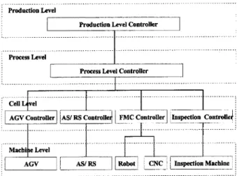
FMSs combine the advantages of the high-flexibility job shop production and the high-efficiency flow shop production. Thus, FMSs can be designed to produce multiple types of components in small batches. The FMS under study will be decomposed into four levels hierarchically as shown in Fig. 1. 1. Production level. This is the highest level in an FMS. It handles the operations of the system, and it consists of a master production schedule (MPS), system resource manage- ment, database, scheduling of maintenance and system performance measurement.

2. Process level. This coordinates and controls all cells in the FMS, e.g. real-time scheduling (dispatching) rules.

3. Cell level. This is the level of the manufacturing cells below the process level.

4. Machine level. This may be machining, inspection or

material handling equipment, e.g. conveyors, machining centre, lathe machine, milling machine, inspection centre, robot and automated guided vehicle (AGV).

3. Modified Coloured-Timed Petri Net

(MCTPN)

The MCTPN extends the framework of the original PN by adding colour, time and modular attributes to the net. The

Production Level

I Production Level Controller J

Process Level

Process Level Controller [

i

. . . ... ../,.j_

:'Cell vel . . .

!L

AGV Controller I [;SIRS Controlle.~ IFMC Control le~r [Inspection C ontrolle! i

iiiiii@ i ii i i iiiiiiiiiiiii iiiiiiii:ii::

! ... 1

.t A o , 1[ AS, SS

i ...

Fig. 1. Hierarchical structure of the FMS.

colour attribute [1-4,13,14] is developed to tackle large systems that have many similar or redundant logical structures. The time attribute [1.4,14] allows various time-based performance measures to be conducted in the system model. A time-delay can be assigned to either places or transitions to model the time properties in a system.

In a PN, when a token in an immediate place is enabled, the condition of the output transition determines the fate of the token. If the output transition is an immediate transition then the enabled token fires and escapes from the input place. In the meantime, the transition releases this token to the output place(s). On the other hand, if the output transition is a timed transition, then the token will not be fired until a prescribed time delay is reached. Tokens in a timed place are processed in a similar way.

Notice that the number of arcs between the input place(s) and the output transition(s) is also important to the token. Three types of arc are used; namely, directed, inhibitor and interrupt arcs. The directed arc connects a place to a transition, or vice versa. It has no preconditions associated with it. The inhibitor and interrupt arcs are defined as follows. The place connected with the inhibitor arc is called the inhibitor place. When the inhibitor place contains the same colour token as the output transition, then the output transition is inhibited from firing. Similarly, the place connected with the interrupt arc is called the interrupt place. When the interrupt place contains the same colour token as the output transition, then the firing of the output transition is interrupted and further inhibited. For the immediate transition case, the inte~upt and the inhibitor arcs behave in the same way. For the timed transition case, the interrupt and the inhibitor arcs do not behave in the same way. If the timed transition is firing and the interrupt place has the same cotour, then it interrupts the firing of this transition and returns the colour token to the input place(s) [2-6,14].

Modular design is essential for a compact FMS model. In addition to the four levels mentioned above, each level is subdivided into several subsystems in a similar fashion, For example, the ceil level under study consists of an FMC1 and FMC2. To facilitate modular design, individual modules are developed first for each of the four levels. Then, the modules for different levels are integrated to form the complete FMS model.

In this iapproach, macro transitions are often used to realise a modular design [1-6,14,15]. A macro transition is the combination of a series of transitions, places and arcs. A macro transition may consist of several submacro transitions (it is, in essence, a macro transition but at different levels). A system can be composed of many macro transitions. The intercon- nection between different levels is achieved by communication places. Based on macro transitions and communication places, a hierarchical and modular model of the FMS can be constructed. The communication and interface between the macro transitions are achieved using four types of communication place, i.e. pitch-up, pitch-down, catch-up and catch-down places. The pitch-down and catch-down places are applied to the higher- level modules, and the pitch-up and catch-up places are for the lower-level modules. The higher-level modules use the pitch-down place to send (or pitch) tokens to the lower-level

(3)

M C T P N for Modelling FMSs 739 modules, and use the catch-down place to receive (or catch)

tokens from the lower-level modules. Similarly, the lower-level modules use the pitch-up place to send tokens to the higher- level modules, and use the catch-up place to catch tokens from the higher-level modules [2-6,141.

By using a hierarchical and modular design, the FMS can be modelled modularly. The primary considerations are to make the model easy to extend, maintain and debug in the future. A hierarchical MCTPN is a ten-tuple, M C T P N = (P~,T~,Po, To,P~,T,,A,B,F,C), where P, is a set of timed places; T~ is a set of timed transitions; Po is a set of immediate places; To is a set of immediate transitions; Pc is a set of communication places; T,,, is a set of macro transitions; A is a set of directed arcs; B is a set of inhibitor arcs; F is a set of interrupt arcs; C is the colour set of transitions and places.

These elements are further elaborated as follows:

1. Place: P = {pl,p2,p3,...,pn} is a finite set of places, n -> 1, including immediate places, timed places and communication places. Notice that the immediate places describe the conditions or properties (without time factor) of resources; the timed places describe the time properties of resources; the communication places describe the communication packages in the hierarchical MCTPN.

2. Transition: T = {tl,t2,t3,...,tm} is a finite set of transitions, m-> 1, including immediate transitions, timed transitions and macro transitions. Notice that the immediate transitions describe the behaviours or events (without time factor) of resources; the timed transitions describe the time properties of resources.

3. Colour: C(p) and C(t) represent the colour sets of places in P and transitions in T;

C(p~) = {a~,,ai2,...,a~,i}, u~ = [C(pl)] (i = 1,2,...n) c( 0 = {bj,,bv~,...,bj,~}, v, = Ic(oi q = 1 , 2 , . . . , m )

where n and m are non-negative integer; a and b are colours of places and transitions, and ] • [ denotes the cardinality. 4. Input, output, inhibitor and interrupt functions:

I(p,t)(a,b) : C(p)xC(t) --* N, is an input function. It describes the mapping relation from the transition t with colour b to the place p with colour a, where N is an non-negative integer. Similarly,

O(p,t)(a,b): C(p)xC(t) ~ N, is an output function Inh(p,t)(a,b): C(p)xC(t) ---, N, is an inhibitor function Int(p,t)(a,b): C ( p ) x C ( t ) ---, N, is an interrupt function 5. Marking: Ix(p):C(p) ~ N; V p ~ P , has n elements, tx(p~) is

an (n x 1) vector defined as:

u t

IX(Pi) = ~nihai,,,

h = I

where nih is the number of colours aih at this instant; u; is the total number of colours in place p~. The term Ix(p0(aih) denotes the number of colours aih in place pi. The term IXo is the initial marking.

6. Conditions of enabling and firing: The transition t~ is enabled with respect to the colour bj, if

ix(pi)(alh) ~ l(pi,O)(a~h,b~,), V Pi E P, au, E C(pi) Ix(pk)(akg) = O, Vlnh(pk,t~)(akg,bjk), V Pk ~ P, ak,~ ~ C(Pk)

Ix(pl)(a¢) = O, VInt~@)(a~bjk), V Pl ~ P, ag E C(p,) After the transition tj is fired, there are two possible out- comes.

For an immediate transition the new marking ix' becomes: Ix'(pi)(ai~,) = tx(Pi)(aih) + O(Pi,tj)(aih,bjk) -- l(pi,tj)(aih,b~k) For a timed transition, the temporary marking I~' is:

Ix'(p,)(a~t,) = p~(p~)(a~,,) - I(p~,tj)(a,h,bjk)

The transition waits for the firing time, then releases the token(s) to the corresponding place(s).

Then the new marking ix" becomes: ix"(pi)(aih) = ix'(pi)(ai,,) + O(pi,ti)(aih,bjk)

7. Time function: It is simply the time attribute in the places and transitions. For the transition, f(t(bjk)): T ~ N, is the time required by the timed transition t associated with the colour bjk to complete the firing. For the place, f(p(ai~)): P N, is the time delay required in the timed place p associated with the colour aih to release.

8. Reachability set: It consists of all reachable markings from the initial marking.

9. Liveness, deadlock: For any reachable marking, if there exists a transition in this MCTPN which is enabled, then the MCTPN is live; otherwise, this MCTPN is in a deadlock.

The icon definition of MCTPN is shown in Fig. 2.

4. Object-Oriented MCTPN Description

The object-oriented technique is becoming more popular for system modelling and analysis, especially for software application development. The object-oriented approach describes the system as a collection of objects, and these objects can interact with one another using both data structure and behaviour. Thus, object-oriented technology attempts to connect the data

O O

©

Place Catch-Down Place Pitch-Down Place

O @

©

Timed Place Catch-Up Place Pitch-Up Place

Timed ~ Macro

Immediately Transition Transition

Transition O T o k e n - > A r c - - - - o Inhibitor Arc - = Interrupt Arc

(4)

740 C-tl. Kuo et al.

and behaviour strongly. In the object-oriented area, the aspects are identity, classification, polymorphism, and inheritance. In the design of a system, the methodology binds the model in the application domain, then implements this system in detail. The methodology consists of analysis, system design, object design, arid implementation stages [11].

In this study, the object-oriented MCTPN models are designed in terms of the stages of object-oriented methodology. Class, message and object are elements of object-oriented technology. In the object-oriented approach [16] object and message passing represent the resource object and the relationship between the resource objects. Class and inheritance can reduce the effort required for system development. The method represents the operation of the objects. Thus, MCTPN objects may be described by using the object-oriented description.

Aggregation, generalisation and inheritance play important roles in the design of an object-oriented MCTPN FMS model. Aggregation can be described as the relationship of "part- whole" or "a-part-of". In other words, aggregation describes the relationship between an entire assembly object and its component objects. Generalisation and inheritance can be used to share the similarities among classes while preserving their differences. In other words, generalisation describes the relationship between a class and its refined version. The class being refined is the superclass, and each refined version is a subclass. Since the instance of a Subclass is also an instance of the superclass, generalisation may be described as the relationship of "is-a" [10]. In the object-oriented MCTPN FMS models under study, the applications of aggregation and generalisation are described as follows:

1. The system view: In the FMS under study, FMC1 and

FMC2 are two manufacturing cells. The manufacturing cell, storage cell, inspection cell and AGV are parts of the FMS. Thus, aggregation association can represent the system object architecture of FMSs (see Fig. 3).

2. The object-oriented M C T P N view: In the object-oriented MCTPN under study, the MCTPN objects are constructed by using the inheritance association. Within the object hierarchy, subclasses inherit or override attributes from its superclass, and the branches from a class are its subclasses. Thus the classes of places and transitions can be classified to be the superclasses in MCTPN nets (see Fig. 4). An MCTPN model can represent the dynamic behaviour of the object-oriented model. The colour sets of an MCTPN

FMS

1 Aggregation = "a-part-of'

~ @ G ~ z a t i o n

= ' ' a - ~ d - O P ' ~

Fig. 3. Aggregation and generalisation of an FMS.

I

Inspeetio

G2 Object

- -- Places "W"- Immediate

"-"I"- Immediate

Unit

Token Place

Place L

Multiple

Token

Immediate Place

/

Timed

Unit

Token

~

Place ~

Timed

Place

Multiple

Token Timed Place

L 7?a onioatio Uii' Token

Communication

Place

Unit Token Pitch Up

Place

Unit

Token Pitch Down Place

Unit

Token Catch Up Place

Unit

Token Catch Down Place

Multiple

Token

Communication

Place

f Multi-Token Pitch Up

Place

Multi-Token Pitch Down

Place Multi-Token Catch Up Place

Multi-Token Catch Down

Place

- Transistions---T--- Immediate Transition

L _

_{Timed Transition}

Message Arcs Directed

Arc

Passing

- ~

Inhibitor Arc

k _ _ Interrupt Arc

Container

Macro

Transition

Fig. 4. The MCTPN object hierarchy.

definition indicate the attributes of places and transitions objects. For example, a timed place may have attributes such as boundedness, time, job, batch, buffer and machine attributes. The messages are transmitted by the arcs connecting the places and the transitions. The transitions are mapped into the operations in the MCTPN nets.

Modular design can simplify a complex FMS model. A macro transition can describe a series of actions for places and transitions. It is a modular representation. Container [16] is an important property in the object-oriented approach, and it allows objects to be embedded within it (for example, Microsoft Word). In the object-oriented MCTPN approach, the modular MCTPN can be described, that is a macro transition can be described as a container. For example, there are several place objects and transition objects in a container, and such a container is a modular design. The container tree of this FMS is described in Fig. 5.

When constructing an object-oriented MCTPN, the MCTPN objects can be described as:

1. Transition objects describe the event or decision. 2. Place objects describe the resource or condition.

3. Arcs describe the message passing; they are the operations between objects.

FMS

FMC T " FMCI -]--- Lathe (Modular with MCTPN Objects)

L

/

~

Milling (Modular with MCTPN Objects)

Robot (Modular with MCTPN Objects)

FMC2 (MC) (Modular with MCTPN Objects)

-- ASRS (Modular with MCTPN Objects)

-- AGV (Modular with MCTPN Objects)

-- Inspection Center (Modular with MCTPN Objects)

(5)

MCTPN for Modelling FMSs 741

Fig. 6. FMC and cell controller.

Fig. 9. FMC1 layout. ' I S P [ A Y I [d( Fig. 7. FMS layout. m I + ' ~ ' + k C ~ l ° I I F u + r ' ~ E ~ S E O I ~ I t ~ + ~ ° l ~ I ~ I r " + + ' + + m l ,+ I lFi"i=h+a~mhNoi+ I S T ~ I ~ a STArI~Z S r A T I ~ STATIO~ I,'=1 + I J 1~ A 1o IN 1 ~ ~ L AS~S ) ~ [ ~ AGV STATIO~ I I+~*°+ I " I ~YSTE~L EFT'TPIE ~ , A I I ~ AGV pARKING STATIONS

Fig. 8. FMS layout for the real-time simulator.

4. Macro transitions may be described in terms of containers. An object-oriented MCTPN has the following properties: 1. MCTPN class hierarchy and inheritance.

TIME-LEFT-OF-LATHE ROBOT

I T+"+"°'~+~°l 2~ I

TIME-LEFT-OF-FM01

Fig. 10. FMCI layout for the real-time simulator.

I To,+.°,k,..+ 1,761

TIME-LEFT-OF-MILUNG

2. Generalisation of MCTPN instance objects from MCTPN classes.

3. Data abstraction.

4. Collaboration among objects. 5. Polymorphism.

6. Dynamic binding.

Thus, the encapsulation, inheritance and polymorphism properties of object-oriented technology help designers to model a complex FMS conveniently. In addition, the reusable property of object-oriented technology reduces software development time. In this study, object-oriented technology and modular design can make system modelling and the simulator coding much easier and faster.

Since the properties of the object-oriented modelling (OOM) are used to model an FMS with the class, object and container trees, software IC will be possible when modelling the FMS.

(6)

742 C.-H. Kuo et al.

Particularly, the developers need only to consider the interfaces and operations relating to the defined MCTPN objects.

In practice, the MCTPN classes must be constructed first. All objects of immediate places, timed places, communication places, immediate transitions, timed transitions and macro transitions are created from the instances of the con'esponding MCTPN classes. In this manner, a complete MCTPN net can be transformed into an object-oriented program. Thus, an object- oriented description MCTPN model and an object-oriented programming can be realised.

5. Modelling an FMS by Using MCTPN

Before modelling the FMS, the designers have to construct the MCTPN classes, then group then into the class libraries. In this paper, the structure of the FMS is decomposed into four hierarchical levels. The MCTPN model is built using modular design. Each module of the MCTPN model is based on macro transitions. The material and information flows in the FMS are integrated by the communication places. The following concepts are used in the modelling of an FMS:

1. An immediate place describes the resources of the FMS, such as material, machine, message, control command and buffer.

2. A timed place is used to model a place that is associated with a time-delay, for example, a conveyor belt on which components stay for a certain time.

3. A communication place describes a place that provides communication between macro transitions, e.g. between a cell layer and a machine layer.

4. An immediate transition models the events occurring in the 1~3,IS, for example, a machine completes one job. On the other hand, it can also model decision making, such as selecting the next product type for a machine under a specific dispatching rule.

5. A timed transition can describe a process that needs time to complete.

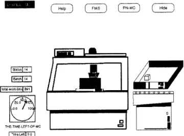
Fig. 11. FMC2 layout.

NNvr]

I,o,~ork~im4 B;! I

THE-]]ME-LEFT-OF-MC

Fig. 12. FMC2 layout for the real-time simulator.

Fig. 13. AGV and AS/RS layout.

6. A macro transition models the aggregation of many processes, such as the cells or machines.

The following procedures are used in the construction of the model:

1. Analyse the FMS, use the hierarchical construction, and define the cells and machines in each level.

2. Define the system requirements, resources, decision making and events, then describe them using appropriate places and transitions.

3. Use macro transitions to model the FMS, cells and machines. Modify them in different levels if necessary. 4. Define the processes in each level in terms of material flow

or machines.

5. Draw flowcharts of the processes in step 4.

6. Define the interface and communication between different levels and macro transitions.

7. Use MCTPN to model the flowcharts in step 5. 8. Justify the model.

This approach will be implemented on an object-oriented real- time expert system, G2 [17]. The G2 environment provides an

(7)

LgilLILlI ilr J]r ln

CART _p'~pr3

Fig. 14. AS/RS layout for the real-time simulator.

inference engine to reason about the objects in the knowledge base. The object-oriented description MCTPN model can be constructed easily in such an object-oriented real-time expert system.

6. Dispatching Rules

So far, the approaches described above can only construct the FMS MCTPN model. However, such an MCTPN model cannot run alone. In this paper, dispatching rules are also proposed. An efficient dispatching rule affects the system performance directly. Thus, this MCTPN model can be integrated with some efficient dispatching rules to operate this simulator. In such a way, a complete real-time FMS simulator is achievable. In this paper, 13 real-time dispatching rules are used. In the MCTPN model, the dispatching rules are added to transition decisions. The dispatching rules are developed in terms of the workpiece characteristics and machine characteristics. Thirteen dispatching rules [3,6] are developed as follows:

1. Dispatching rules depending on workpiece characteristics: (a) "FCFS": first come first serve.

(b) "SPT": shortest processing time.

(c) " W S ~ " : weighted shortest processing time. (d) "SRPT": shortest remaining processing time. (e) "LRPT": longest remaining processing time. (f) "FORT": fewest operation remaining time. (g) "LORP": largest operation remaining time. (h) "EDD": earliest due date.

2. Dispatching rules depending on machine characteristics: (a) "SOTA": shortest operation time with alternative con-

sidered.

Fig. 15. Inspection unit.

kE FT÷T[ME ~ F 4 N ~ E G ~ ~

Fig. 16. Inspection cell layout for the real-time simulator.

(b) "ESTA": earliest starting time with alternative considered.

(c) "LITA": longest idle time with alternative considered. (d) "EFTA": earliest finishing time with alternative con-

sidered.

(e) "I]ITA" + "ESTA": combination of "LITA" and "ESTA".

(8)

744 C.-H. Kuo et at.

7. Application Examples

The proposed MCTPN will be used to design an FMC controller and an FMS simulator. The real-time cell controller for the FMC, based on the MCTPN, is shown in Fig. 6. This FMC contains a cell controller, a D&M4 CNC milling, a pallet, a CNC lathe (a simulation stand), a storage unit, a conveyor, a mini robot and some workpieces. The cell controller can control this FMC by using some appropriate dispatching rules. The real-time controller is constructed using the MCTPN model. A graphical user interface (GUI) is also developed for monitoring and simulation purposes. The GUI and cell controller are implemented on a personal computer.

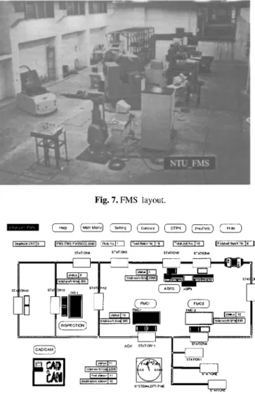
A real-time simulator for the FMS is developed to illustrate how to create and implement the MCTPN model. Thirteen dispatching rules are used to operate this FMS real-time simulator. This FMS plant is an experimental automated factory in MATRC, National Taiwan University (see Fig. 7). It includes a transportation cell, a storage cell, two FMCs and an inspection cell. In this simulator, the graphical user interface plays

an important part. Figure 8 shows the simulator layout. The cells are described as follows:

t. FMCI: is the first manufacturing cell in this FMS, and consists of a CNC milling machine, a CNC lathe machine, a robot and two buffers. Figure 9 shows the FMCI layout, and Fig. 10 shows the FMC1 layout of the real-time simulator.

2. FMC2: is the second manufacturing cell in the FMS, and consists of a machining centre and an automated pallet changer and two buffers. Figure 11 shows the FMC2, and Fig. 12 shows the FMC2 layout of the real-time simulator. 3. Transportation cell: includes an AGV and three parking

stations. The AGV is shown in Fig. 13.

4. Storage cell: consists of an AS/RS that is a three-by-six unit warehouse, a cart and two buffers. Figure 13 shows the AS/RS layout, and Fig. 14 shows the AS/RS layout of the real-time simulator.

5. Inspection cell: includes a coordinate measuring machine (CMM) and two buffers. Figure 15 shows the inspection

1

i

I

I i I I

I

k~,

Inspe0~on

A,.C4tqS

Gomn'~nd

~ P M $ . F 2

AGV upb~.~ab~

:.,22,,

PM~_PI

P]oces,s

RV,~

_TS

f~Mg_P

t7

1 AS RS.BF

ASRS-Room

[<

INSPECTION

V j/

FMC

R~ST6

FMG

'1

H f~t$_T44

~

'O P-S.~S

i

FMC.

M

~ted~:in ;

Fig. 17. MCTPN for FMS.

(9)

'1" ~, FMC~ T'~ upl~d F'M~ Pe _pt~ ~C~ CNC I ~ ] ~ T ~ I t41 ~..plG) Fr~o_~t W/,O,.p~ ~ ~ ~ a.rmad FIdC-BF (rm.%p~) + F'I~.II ~ F'k~ _PaR Fig. 18. MCTPN for FMC1. MCTPN for Modelling FMSs 745 (o~_pe) r~*o..Pm _pig) u p l ~ rob_p~) I~o_p~) FllO..PI6 m m ~ ~ b_l~7~ _ol)

unit layout, and Fig. 16 shows the inspection cell layout of the real-time simulator.

A graphical human machine interface (GHMI) [2] is intro- duced to simulate this real-time FMS simulator. The operator can set up the following conditions:

1. Set up the number of workpieces in each batch, the maximum number of batches is eighteen.

2. Set up the routeing steps and processing times for every batch.

3. Set up the due date of every batch. 4. Set up the weighting of each workpiece.

5. Set up the performance (or reliability) of all machines and cells.

6. Set up the dispatching rule that can operate in this real- time FMS simulator.

7. Set up the run mode with the options of one shift only or 3 shifts (continuous production).

In addition to the GHMI, some functions are also provided in this real-time FMS simulator. These functions are the real- time monitoring of FMS activities, real-time monitoring of MCTPN activities and on-line performance queries. The man- agers and operators can examine this system for process monitoring, and the process engineers can evaluate this system for both process monitoring and MCTPN emulation.

The following steps are used to model an FMS by using MCTPN.

1. Define macro transitions in the system level: they are AGV-macro-rransition, AS/RS-macro-transition, FMC-macro- transition and inspection-macro-transition.

2. Define the macro transition in the level of FMC-macro- transition: they are FMCl-macro-transition and FMC2- macro-U:ansition.

3. Define the macro transition in the level of FMCl-macro- transition: they are CNC-macro-transition and robot-macro- transition.

4. Define the decision transition in the system level. (a) Materials input system.

(b) Materials output system.

(c) Materials begin processing from AS/RS. (d) Materials begin inspecting from AS/RS. (e) Materials begin processing from the other cell. (f) Materials begin inspecting from the other cell. (g) Material back to AS/RS.

5. Define the decision transition in the cell level of FMC1. (a) Robot uploads the job.

(b) Robot transfers the job. (c) Robot downloads the job.

6. In the machine level, analyse the necessary activities of a machine, and list all the required commands. The developers can describe them using appropriate places and transitions, and model the processing time by using the timed transitions.

7. Finally, define the communication places in the system, cell and machine levels.

For the proposed FMS, 13 dispatching rules are provided. These dispatching rules are provided in terms of the job properties and machine properties.

(10)

746 C,-H. Kuo et at. Itm~.da~t 1 ~ " ~ ~

,@

mo~ ~ W J O~ OWO_T ONO_TS ONO.Tt;~ ONO.PI ~ ~ ONO.Pt6 Fig. 19. MCTPN for CNC.

The complete b ~ S model can be constructed by using MCTPN. In the system level, there is an MCTPN net for FMS (see Fig. 17). In this net, transitions are used to describe the events, decisions, and macros in the FMS layer. For example, the FMS_T1 decides the destination cell, destination buffer, and the extracted workpiece in the AS/RS; the FMS_T14 describes the event of workpiece return to the AS/RS; the

ES

Set up initial token I

+

Find all the places thatL~ I have received tokens l -

System deadlock ~ Ctt~sii~.o°t?nt

handling .... I I [_

Cheek end ~ Echo the enabled

of simulation I - [ transition

YES I Timed _{transition j~ find firable transition [ [}I J l Check confliet and

Fi ngof med']

[transition complete] Immediate [ transition "~J ,,,I <2 / 1, Release token K J New marking 't / /

Fig. 20. Simulation flowchart for firing MCTPN.

FMS_T11 describes the behaviour of the inspection cell. Places are used to describe the commands, resource status, and communication packages. For example, the FMS_P2 describes the command of "input" or "outpuf'; the FMS_P22 communicates with the inspection cell; the FMS__P7 describes the status of AGV.

In the cell level, there are MCTPN nets for FMC1, FMC2, AGV, AS/RS and inspection cells. Here, an example of an FMC1 MCTPN net is shown in Fig. 18. On the lefthand side of this net, there are two macro transitions (robot and CNC). Each macro transition describes the behaviour of the corresponding machine. The communication places can communicate with the higher and lower layers. For example, FMC_P1 can receive FMS messages; FMC_P6 can send messages to the CNC. On the righthand side of this net, there are several nets. These nets contain the communication between the higher and lower layers.

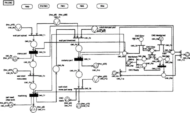
In the machine level, there are MCTPN nets for CNC machines and the robot. The CNC MCTPN net is shown in Fig. 19. In this net, the timed transition is used to describe the process of action. For example, CNC_T7 describes the process of machining; CNC_T14 describe the process of maintenance. When the MCTPN nets for the FMS have been completely constructed, the designer can write a program to simulate the FMS by using these MCTPN nets and the constructed MCTPN class libraries. In addition, the modular design and object- oriented programming (OOP) can simplify the coding work. In this FMS under study, a real-time object-oriented expert system G2 is used to establish this approach and simulate this FMS. The simulation flowchart is shown in Fig. 20.

The functions of this real-time simulator are described as follows:

1. Man-machine interface: including workpiece data setting, the workpieces of each batch, the routeing and processing

(11)

Table 1. Batch data setting.

Batch number Process 1 Process 2 Process 3 Process 4 Process 5 Total job number (time) (time) (time) (time) (time) in one batch 1 la(50) lb(45) 3(20) 2(55) 3(20) 1 2 2(70) 3(20) la(45) lb(50) 3(20) 1 3 lb(40) la(60) 3(20) 2(80) 3(20) 1 4 2(65) 3(20) lb(35) ta(40) 3(20) 1 5 2(55) 3(20) 1 6 la(45) 1b(55) 3(20) 1 7 3(20) 2(70) 3(20) 1 8 3(20) lb(45) la(55) 3(20) 1 9 la(45) lb(40) 3(20) 2(75) 3(20) 1 10 2(75) 3(20) la(45) lb(45) 3(20) 1 11 lb(50) la(55) 3(20) 2(70) 3(20) 1 12 2(65) 3(20) la(55) lb(60) 3(20) 1 13 1b(45) la(50) 3(20) 2(70) 3(20) 1 14 lb(40) la(45) 3(20) 2(70) 3(20) 1 15 1a(45) lb(45) 3(20) 1 16 3(20) 2(65) lb(45) la(40) 3(20) 1 17 lb(45) la(50) 3(20) 2(55) 3(20) 1 18 2(70) 3(20) la(45) lb(35) 3(20) 1 where

Process index la: FMC1 lathe Process index lb: FMCI milling Process index 2:FIVIC2 (MC) Process index 3: Inspection centre Time: simulation time unit (second)

• : None operation

time setting for each batch, job weight setting, machine performance index setting, A G V operation rule setting, dispatching rule setting, etc.

2. Display console: including shop floor control [18] and monitoring, M C T P N enumeration, system performance, use, workpiece status, etc.

3. Alarm message board.

4. Gantt chart for the machine and workpiece.

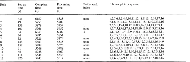
Some results are selected for explanation. Table 1 shows the batch data setting for this simulator. The set-up data provides the initial conditions for FMS production. Table 2 Table 2. Simulation results under different dispatching rules.

shows the simulation results for different dispatching rules, and it also indicates the operation time for different dispatching rules. In addition, the system bottleneck index and the order of every workpiece that completes all processes under different dispatching rules are also discussed. The system bottleneck index shows the risk of having a bottleneck situation in the system when improper dispatching rules are used. This index is measured from the simulation results and it represents the frequency that the system is in a bottleneck condition.

Figure 21 shows the on-line query for the workpiece status. In this figure, the status of every workpiece can be displayed in this workspace. For example, they can be the batch number, Rule Set up Complete Processing

time time time (s) (s) (s)

Bottle neck index

Job complete sequence 1 634 6159 5525 2 49 5758 5709 3 139 5878 5739 4 109 5761 5652 5 34 6043 6009 6 34 5885 5851 7 52 5526 5474 8 148 5683 5535 9 157 5782 5625 t0 61 5549 5488 11 68 5728 5660 12 l l l 5644 5533 13 226 5743 5517 none 1 1 none 3 1 none none n o n e n o n e 1 none none 1,2,7,6,5,3,4,9,10,11,12,18,8,13,15,14,17,16 2,1,6,14,3,4,9,15,13,12,17,18,11,10,7,5,8,16 2,6,5,1,15,4,10,12,18,8,7,16,3,14,13,17,9,11 1,2,7,5,15,6,17,4,14,18,10,13,9,11,3,12,8,16 2,1,12,5,10,4,13,9,14,6,17,16,3,8,15,7,18,11 1,2,7,5,6,15,4,10,9,12,18,8,3,11,13,14,16,17 1,2,4,3,9,10,12,5,11,18,13,14,17,6,7,16,15,8 2,1,5,15,18,11,4,10,17,8,12,7,3,6,13,16,t4,9 1,2,7,6,5,4,3,10,9,11,12,18,8,13,15,14,17,16 1,2,5,6,4,3,10,9,12,18,7,8,11,13,15,14,17,16 2,1,6,5,4,9,11,13,10,14,15,17,12,18,7,3,8,16 2,1,6,5,3,4,9,10,11,12,18,7,8,13,14,16,15,17 2,1,6,5,3,4,9,11,13,10,14,15,12,17,7,18,8,16 Where rule 1 to rule 13 are the dispatching rules in this study.

(12)

748 C.-H. Kuo et aL

I

present simulation tim e 15526 J batch process fmcl duetime tota}-t job 1 1 0 0 8000 190 job 2 2 o o eaoo 2us job 3 3 0 0 7500 ; 220 iOb 4 4 0 0 7300 180 job 5 5 0 0 7000 ) 75 ~b 6 6 0 o 8000 t20 )ob 7 7 0 0 7500 110 job 3 9 0 0 7300 140 lob 01 9 o o 9000 200 job 101 10 0 0 7500 20~ job 11 I 11 0 0 7000 215 i job 12 12 0 0 8000 220 ob 13 13 O 0 7700 205 job 14 14 0 0 8300 195 job 15 15 0 0 7000 I I0 job 16 ) 16 0 0 7800 lg0 190 job 17 17 0 0 7300 job 18 18 ) 0 0 6700 t90 ) bat: batch n u m b e r for this job

process: incomplete cell process for this job f m c l : l m c l incomplete process for this job

ulil: job processing time t total processing time

total4: FMS total processing time for this job

slate: proce~ state for this job

@It-t: incomplete processing time tor this job

NNe wait-t wor~t NIl FMCI -1 5336 100 0,034 95 -1 5321 205i 0.037 9,5 -1 5306 220! 0.04 ~00 -1 5346 180 0.033 75 -I 5451 75 0.014 0 - i 5486 120i 0,022 100 -1 5416 110 0.02 0 -1 5386 140 0.025 i00 -I 5326 200; 0,036 85 "1 5321 205 0.037 90 -1 5311 215 0,039 105 -1 5306 220 0.04 115 -1 5321 205 0,037 95 "1 5331 195 0.035 85 -1 5416 110 0.02 90 "1 5336 190 0,034 85 *1 5336 190 0,034 95 - 1 5336 190 0.034J 80

work-tim e: job work tim e

duatime: duetime for this job FMCI: trr¢l F o c o s s need lime FMC2:line2 F o c e s s need time

wait4: job wail time

weight: weight Ior this job b-due: time before duetime

Fig. 21. Workpiece status.

FMC2 lefl-t 55 0 70 0 80 0 65 0 55 0 0 0 70 0 0 0 75 0 75 0 70 0 65 0 7o 0 7O 0 0 O 65 0 55 O 70 0 state 1: t m c l 2:frnc2 weight b-due 5 2474 5 1274 6 1974 7 1774 7 1474 6 2474 6 1974 7 1774 4 3474 8 1974 3 1474 4 2474 5 2174 5 3274 6 1474 7 2274 5 t774 4 1174 @ @ inspection center

O: ca'nplete all process

-1: job in ash's and complete a l process

total operation time, waiting time, use, remaining time before completion, due time, weighting and the time before due time. Figure 22 shows the on-line query for the Gantt chart for all cells in the FMS. The operation status of each cell can be seen immediately from this chart. For instance, one can check which workpiece is being processed in FMC1 on a real-time basis. The vertical axis indicates the cells, which are AGV, AS/RS, FMC1, FMC2, and inspection cells. The horizontal axis indicates the simulation time in seconds. The rectangular areas in this figure indicate the workpieces being processed in the corresponding cell, shown with different colours. Notice that the symbols of "FMS-JOBi", i = 1,2,...,18, are the names

I~ FMS*JOB2

,o,'B

If II |

I Iz::;:

FM-S,JOBS I~ FMS-JOB7 FMS-JOB8 FM8 JOB9 I~ FMS 401~I I PMS-J0812 , FMS~IOBI 3 I ~ FMS*JOBI 4 FMQ2 [ , [ I FMS~JOBI~ Inspe¢Son ~ FMS-JOB17 t I ~ FMS-JOBi8

These Datas Will Be Updated Every 650 simulation lima (sec)

Fig. 22. Gantt chart for the workpiece status (cell layer).

Robot Milling LaLhe I I FMC-JOB1 I FMC,.JOB2 t FMC.J083 FMC~JOB4 FMC-JOB5 [ j I F.o.~o~ , ~ FMO-J087 U F~40-,K388 @ F~c JO~9 I FMO-J0811 } FMO.JOB14 , I FMO-JO815 ~ FMO40Bi6 FMC-JOBI7 N FMC-JOB~ I '~

I.~MS-n~E-PASS~DI~7t The.seDelesWi~B,aUpdatedEv~r1650simulationN'nt, (see)

Fig. 23. Gantt chart for the workpiece status (machine layer in FMCI).

of workpieces, which may refer to the different process routines and products in this case. Figure 23 shows the on-line query for the Gantt chm't for all machines in the FMC1. The status of each machine can be found from this chart. For example, one can see immediately which workpiece is being processed on the lathe. The vertical axis indicates the machines in FMC1, they are robot, milling, and lathe. The horizontal axis represents the simulation time in seconds. The rectangular areas in this figure indicate the workpieces being processed in the con'e- sponding machines shown with different colours. Figure 24 shows the on-line query for the Gantt chart for atl workpieces

(13)

job1 lob2 i °b3 ~ GANTr-AGV iOb4 _I [ ] GANTT-ASR 1oD5 } ~[~ c, Am"r.Roe lob7 j0b9 ~ G~',~I'-INSPECTION joblO ,oo,z [] [] ,o.,3 [] jobl4 lob15 jObl6

I

jobl7 ion, E l

I FMS'TIME'PASeEDI ~451 I These Data8 WIll Be Updated Every e5o stroll ~ion time (scc)

Fig. 24. Gantt chart for the machine status.

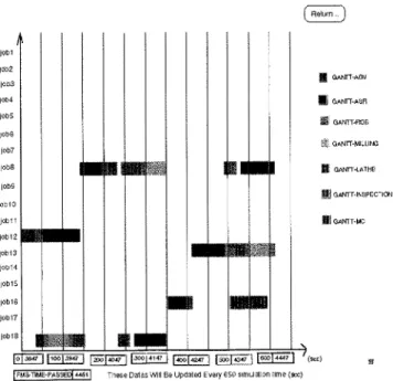
in the FMS. The status of every workpiece can be seen from this chart. For example, one can see which cell or machine is processing a specified workpiece. The vertical axis indicates the workpieces, which are from job1 to jobl8. The horizontal axis represents the simulation time in seconds. The rectangular areas in this figure indicate the processing machines for the corresponding workpieces, each shown with different colours. Notice that the symbols for the workpieces (FMS-JOBi, FMC- JOB/, job/, i = 1 to 18) in Figs 22, 23, and 24 are different, although they describe the same workpieces (workpiecel to workpiecel8). The routeing definitions of all the workpieces are listed in Table 1.

8. Conclusions

In this paper, an MCTPN is proposed for constructing the dynamic activities of FMSs. The proposed MCTPN can be used to design both the FMC controller and FMS simulator. The objective of this paper is to illustrate the procedures of modelling, simulation and real-time control of the FMC and FMS. In the proposed MCTPN, object-oriented description and modular design play important roles. Such an approach can reduce the development time of the system. Any complex system can b e modelled using the MCTPN in this manner, and the models are clear and easy to extend, modify and debug. In addition to the MCTPN modelling of the production activities in the FMS, the failure of machine and maintenance of equipment are also considered. The proposed MCTPN can also be used to model statistical process control (SPC), machine fault, maintenance of equipment and fault diagnosis [4]. Reliability analysis of the FMS based on MCTPN is currently being developed.

MCTPN Jbr Modelling FMSs 749

Acknowledgments

This work was partially supported by the National Science Council, Taiwan, ROC, under Grants NSC85-2212-E-002-073, and NSC85-2622-E-002-018. The authors are grateful to the reviewers for their careful reading of the manuscript and their helpful suggestions.

References

I. H. P. Huang and P. C. Chang, "Specification, modelling and control of a flexible manufacturing cell", International Journal of Production Research, 30(11), pp. 2515-2543, 1992.

2. H. P. Huang and Y. H. Tseng, "Modelling and graphic simulator for integrated manufacturing systems", Proceedings of Intelligent Automation and Soft Computing, 1, pp. 183-186, 1994.

3. C. H. Kuo, "Application of reliability and equipment maintenance to flexible manufacturing systems", Master Thesis, Department of Mechanical Engineering, National Taiwan University, 1995. 4. C. H. Kuo and H. P. Huang, "Colored timed Petri net based

statistical process control and fault diagnosis to flexible manufacturing systems", IEEE International Conference on Robotics and Automation, New Mexico, vol. 4, pp. 2741-2746, April 1997. 5. Y. H. Tseng, "Modularized modeling and simulation of a flexible

manufacturing system", Master Thesis, Department of Mechanical Engineering, National Taiwan University, 1.993.

6. M. C. Yeh, "Development of shop floor control system for flexible manufacturing systems", Master Thesis, Department of Mechanical Engineering, National Taiwan University, 1994.

7. A. A. Desrochers and R. Y. A1-Jaar, Applications of Petri Net in Manufacturing Systems- Modeling, Control, and Performance Analysis, IEEE Press, New York, 1995.

8. S. S. Lu and H. P. Huang, "Modularization and Properties of Flexible Manufacturing Systems", in M. Cotsaflis and F. Vernadat (ed.) Advances in Factories of the Future, CIM and Robotics, Elsevier, Amsterdam, pp. 289-298, 1993.

9. P. Cord and E. Yourdon, Object-Oriented Design, Prentice-Hall, Englewood Cliffs, NJ, 1991.

10. J. Rumbaugh, M. Blaha, W. Premerlani, F. Eddy and W. Lorensen, Object-Oriented Modeling and Design, Prentice-Hall, Englewood Cliffs, NJ, 199I.

11. J. H. Mize, H. C. Bhuskute, D. B. Pratt and M. Kamath, "Modeling of integrated manufacturing systems using an object-oriented approach", IIE Transaction, 24(3), pp. 14-26, 1992.

12. K. Y. Chen and S. S. Lu, "Integration of Petri-net and object- oriented technology for manufacturing systems control software implementation", Bulletin of the College Engineering, NTU, Tai- wan, no. 67, pp. 109-122, June 1996.

13. P. Huber, K. Jensen and R. M. Shapiro, "Hierarchies in coloured Petri nets", Advances in Petri Nets 1990, Lecture Notes in Com- puter Science, Springer-Verlag, pp. 313-341, 1990.

t4. C. H. Kuo and H. P. Huang, "Dispatching and simulation for highly model-mixed automotive plants", Proceedings of the Inter- national Conference on Automation Technology, Talwan, vol. 1, pp. 423-430, 1996.

15. C. J. Tsai and L. C. Fu, "Modular approach for Petri-nets modeling of flexible manufacturing systems adaptable to various task-flow requirements", Proceedings of IEEE International Conference on Robotics and Automation, France, pp. 1043-1048, 1992. 16. R. C. Martin, Designing Object-Oriented C++ Applications,

Prentice-Hall, Englewood Cliffs, NJ, 1995. 17. G2 Reference Manual Version 4.0, Gensym, 1995.

18. A. Bauer, R. Bowden, J. Browse, L Duggan and G. Lyons, Shop Floor Control System- from Design to Implementation, Chapman and Hall, London, 1991.