Robust Adaptive Beamforming in Cognitive Radio Networks

Robust Adaptive Beamforming in Cognitive Radio Networks

Wei-Chiang Wu

Professor, Department of Electrical Engineering, Da Yeh University

wcwm53@mail.dyu.edu.tw

Abstract

In this paper, we propose an adaptive non-intrusive cognitive radio network based on smart antenna technologies. The cognitive transmitter (CT), which is equipped with antenna array, first estimates and tracks the composite steering vectors of each primary (licensed) user. In what follows, CT forms transmit beamforming to place nulls to primary receivers (PR) based on the estimated spatial signatures. Moreover, we extensively analyze performance degradation caused by spatial signatures mismatch (estimation error) and verify that the proposed robust nulls-steering beamformer can comprehensively alleviate the mismatch effect. Simulation results demonstrate convergence of the proposed gradient-based recursive least squares (RLS) algorithm. Furthermore, we have shown that outage probability can be kept extremely low under appropriate array size, which ensures the practicability of the proposed scheme.

Key words: Cognitive Radio, Non-intrusive, Adaptive nulls-steering, Robust beamforming 1. Introduction

Cognitive radio has recently shown its potential for next-generation wireless communications for efficient utilization of the radio spectrum [1-10]. The growing interest towards cognitive radio stems from its promising features to overcome the spectrum congestion by permitting opportunistic access of licensed bands by cognitive users when the primary licensees are inactive. In cognitive radio system, the secondary users can use the licensed spectrum as long as the primary user is absent at some particular time slots or some specific geographic area. In general, the primary objective of cognitive radio is real time spectrum sensing or awareness in order that the radio spectrum can be efficiently utilized. Most past works [4-11] of cognitive radio premise on “detection and avoidance”: when a secondary user is using a spectral band and a primary user is turned on, the secondary user must detect the primary user’s signal and vacant the channel immediately in order not to interfere primary user’s transmission. Therefore, the cognitive transmitter (CT) cannot access the spectrum simultaneously with the primary transmitter in most existing proposals.

Recently, S. Huang et al. [12] has proposed a non-intrusive cognitive scheme based on transmission beamforming. The design parameters are the beamforming weights at the CT, which is equipped with antenna array. Exploiting transmit beamforming techniques, the aim of a non-intrusive cognitive scheme is “coexistence” rather than “detection and avoidance”. It provides more flexible user access rather than the presently works. Moreover, it exploits the spatial void and thus can further improve spectral efficiency. The basic idea of non-intrusive cognitive scheme includes:

(1) The primary transmitter is not concerned about the existence of cognitive users and will not adapt its transmission behavior.

(2) The CT has to guarantee that its interference to the PR is below a limit or threshold in order to gain access and remain non-intrusive.

The work of [12] only considers one pair of primary users and cognitive users and the respective bearings (directions-of-arrivals) are well-known (within a range) and fixed.

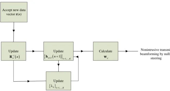
In this paper, we propose a non-intrusive cognitive radio scheme based on adaptive nulls-steering. The proposed methodology is composed of two stages: In the first stage, we develop an adaptive estimator at the CT to estimate and track the composite vector channel impulse responses (VCIR) between CT and each primary user. The rational of the algorithm premise on iteratively maximizing the minimum possible beamformer’s output power. Both the gradient search and recursive least squares (RLS) [13] based methods are exploited to develop the adaptive algorithm. The proposed scheme adaptively tracks possible perturbation of CSI, which in term, taking into account the possible mobility of the primary user in practical cellular networks. In the second stage, the CT exploits the estimated spatial signatures to perform nulls-steering beamforming. In what follows, the interference laid on PRs by CT is zero and both the primary and cognitive transmitters can access the spectrum simultaneously without cancel each other’s transmission.

Though the composite spatial signatures for each primary user (or CSI for the link from CT to primary users) are a matter of vital importance for determining the weights of nulls-steering beamformer, in practice however, there is unavoidable estimation error. We first provide a systematic analysis for the performance degradation induced by mismatch (estimation error). Moreover, we develop a robust downlink beamformer that preserve reliable performance in the presence of mismatch. Since mismatch-induced performance degradation

results from the fact that the nulls-steering beamformer places nulls to the wrong directions. Placing a set of linear constraints to widen and flatten the nulls is impractical due to the limited degrees of freedom (array size). In this paper, we add pseudo noise (diagonal loading) directly on the estimated correlation matrix and exploit it to derive the weight of the robust beamformer. In what follows, the robust nulls-steering beamformer place shallow nulls to the directions of the primary users.

The remainder of this paper is organized as follows. In section 2, we formulate the signal and channel models. Section 3 highlights the rationale of the adaptive algorithm of spatial signatures estimatior. Section 4 describes the design of nulls-steering beamformer. The performance degradation due to mismatch or estimation error and the design of robust beamformer are also extensively analyzed. Simulation results are presented in section 5. Concluding remarks are finally made in section 6.

Notation: The boldface lower case and upper case represent vector and matrix, respectively.

[ ] [ ]

T, H stand for matrix or vector transpose and complex transpose, respectively.

E

[ ]

denotes taking ensemble average on the random variable (vector) inside

[ ]

. “

ˆx

” indicates the estimate of x. I denotes an identity matrix with size _M M. “

≡

” means is defined as.

[ ]

,

i j denotes the element of the ith row and jth column of the matrix inside the

square bracket.

tr

[ ]

means trace (sum of diagonal elements) of the matrix inside the square bracket. e_i is a vector with all entries zero except for the ith entry, which is one.

2. System and channel models

In this paper, we consider an authorized (licensed) communication network which is composed of K users (including one primary basestation (PB) and K-1 primary radio terminals). A cognitive transmitter (we use CT hereafter) attempts to send information to a cognitive radio terminal (we use CR hereafter) within the same geographical region as the primary (licensed) system. In other words, both wireless links are deployed to coexist without deteriorating system performance. Array of antennas with size M is applied both in PB and CT, while single antenna is equipped at each of the radio terminal. Therefore, the signal at the transmitting end can be expressed as

( )

( )

i

t

=

i

s t

x

w

(1)

where

s t

( )

is the information data to be transmitted,

w

_i denotes the weight vector. We use c and p instead of

i to represent cognitive and primary transmitter, respectively. Let

E

{ }

s t

( )

2

=

1

, thus the power consumption is determined by

w

_i 2.

The vector channel impulse response (VCIR) or composite steering vector is characterized by

1 L l l l=

=

∑

α

h

a

(2)

where L denotes the number of paths between the designated basestation and radio terminal.

a

_l

∈

C

M×1 is the normalized array response vector (steering vector) that is parameterized by DOA of the lth path measured relative to the array normal direction.

α

_l accounts for the path loss as well as shadowing effect of the lth path. Please note that in the considered model, we assume that the delay spread is small compared with the bit duration. Hence, (2) only characterizes the azimuthal dispersion and ignores the temporal dispersion. In space division multiple access (SDMA), the basic idea of signal separation is to treat h as unique, user-specific spatial signature.

Intuitively, the non-intrusively cognitive scheme should guarantee that the radiation pattern of CT will have nulls in the directions of primary users. On the other hand, the primary users need not to deal with the existence of all cognitive users. Hence, the problem addressed in this paper is the design of beamformer in CT with two purposes in order:

(1) Spatial signatures estimation of all primary (licensed) users and tracking (adaptive processing) based on the observed vector data sequences.

(2) Design transmit beamformer that steers nulls to all the primary users in order that the performance of PR is not affected by the cognitive link.

3.1 Preliminary

As we have described in section 1, the proposed adaptive non-intrusive cognitive radio scheme is composed of two stages.In the first stage, the cognitive user needs not only to estimate the bearings (DOAs) of all the primary users but also to track them. We deduce and analyze the adaptive spatial signatures estimation algorithm in this section. Assuming that there are K users in the primary network, then the signal received by the array (with size M) of CT can be written as

, 1

( )

( )

( )

( )

( )

K k k cp k k

i

a d i

i

i

i

=

=

+

=

+

∑

r

h

n

CAd



n

(3)

where

a

_k is the amplitude of the kth user,

A

≡

diag a

{

₁

a

₂



a

_K

}

. The ith bit transmitted by kth user is given by

d i

_k

( )

, which takes on

±

1

with equal probability (BPSK-modulated signal is assumed).

[

1 2

]

( )

i

≡

d i

( )

d i

( )

d

_K

( )

i

T

d



.

n

( )

i

is the background noise, under spatially white assumption,

2

( )

H

( )

_M

E



_

n

i

n

i

 = σ

_

I

.

{ }

_, 1, , cp k _{k= K} h

 denotes the effective (composite) spatial signature between the CT and the kth primary user. Based on the model of (2), we may express

{ }

,

1, , cp k k= K h  as

( )

( ) ( ) , , 1

;

1,

,

k L l l cp k k k cp k l

k

K

=

=

∑

α

θ

=

h

a



(4)

where

L

_k denotes the number of paths between the CT and kth primary user.

a

_k

( )

θ

( )_{cp k}l_,

∈

C

M×1 is the normalized steering vector that is parameterized by DOA

( )

θ

( )_{cp k}l_, of the lth path measured relative to the array normal direction.

α

( )_kl is the fading coefficient corresponding to the DOA

θ

( )_{cp k}l_, .

,1 ,2 ,

cp cp cp K





≡ 



C



h

h



h

is a matrix with size

M

×

K

.

We develop the estimation algorithm by applying the rational of the MPDR beamformer[14]. The choice of weight vectors,

{ }

1, , k k= K

w

_ , for the MPDR beamformer aims to minimize the output power,

{

2

}

( )

H H

k k rr k

E w r i =w R w , while distortionlessly passes the desired signal, leading to the following constrained optimization problem

,

arg min

1

k H k rr k H k cp k

subject

to





=



w

w R w

w h

(5)

where

R

_rr

=

E

_



r

( ) ( )

i

r

i

H

_



=

CA C



2



H

+ σ

2

I

_M is the correlation matrix of the observation vector. Using Lagrange multiplier method, the solution of (5) can be obtained as

1 , 1 , ₁ , ,

ˆ

ˆ

ˆ

rr cp k k k rr cp k _H cp k rr cp k − − −

= η

=

R h

w

R h

h

R h

(6) where 1 , , 1 ˆ ˆ H k k rr k H cp k rr cp k − η =w R w =

h R h stands for the output power of the MPDR beamformer at k

w

. Since

only the desired signal is “distortionlessly” passed, the output power of the MPDR beamformer is mainly determined by the desired signal’s power. Consequently, the spatial power spectrum,

( )

1 1 ˆ H rr − η x = x R x, should exhibit K peaks at

{ }

, 1, , cp k k= K = x h

 , respectively. Motivated by the output power degradation due to the mismatch of the primary users’ spatial signatures, we propose to adaptively estimate

{ }

,

1, , cp k k= K h  toward the direction of maximizing

{ }

1, , k k= K η _ , which yields



, , 1 , _{, ,} 1 , ,

1

_ˆ

arg max

arg min

ˆ

cp k cp k H cp k _{cp k rr cp k} H cp k rr cp k − −

=

=

h h

h

h

R h

h

R h

(7)

Incorporating the unit-norm constraint on the spatial signature, we may reformulate (7) as

, 1 , , , , ˆ arg min 1 cp k H cp k rr cp k H cp k cp k subject to −   =  h h R h h h (8)

3.2 Recursive implementation of the primary users’ spatial signatures estimators

Using the method of Lagrange multipliers to solve (8), we first establish the cost function

(

)

1

(

)

, , ˆ , , , 1

H H

cp k cp k rr cp k k cp k cp k

J h =h R h− − λ h h − (9) where λk is the corresponding Lagrange multiplier. The gradient of J with respect to hcp k, gives the search direction for each iteration

(

)

(

)

, 1 , 2 ˆ , , cp kJ cp k rr cp k k cp k − ∇h h = R h − λ h (10)

Upon setting the result of (10) to zero and multiplying both sides by h_{cp k}H_, yields 1 , ˆ , H k cp k rr cp k − λ = h R h (11)

Compare (11) with (6), we can obtain that _k 1

k

λ =

η , the inverse of the MPDR beamformer’s output power.

To accommodate the time-varying characteristics of data vector, we first deduce the adaptation rule for

rr R as

( )

(

)

ˆˆ _{1 ( )} H_{( )} rr n = ς rr n− + n n R R r r (12)

where

ς

denotes the forgetting factor. From the well-known matrix inversion lemma [14]

(

)

_{-1 -1 -1}

(

_{-1 -1}

)

-1 _-1

A + BCD

= A - A B DA B + C

DA

(13)

We arrive at an update equation for R_rr−1

( )

n

1 1 1 1 1

ˆˆ (

1) ( )

( )

(

1)

1

1

ˆˆ ( )

(

1)

ˆ

( )

(

1) ( ) 1

H rr rr rr rr _H rr

n

n

n

n

n

n

n

n

n

− − − − −

−

−

=

− −

ς

ς

−

+

R

r

r

R

R

R

r

R

r

(14)

The iterative equation for

{ }

, 1, ,

cp k k= K

h

 can be obtained using classical steepest descent algorithm [13]. Thus, at the (n+1)th iteration, the estimate of h_{cp k,} can be obtained as

(

)

(

)

, , , 1 , , , 1 , , ˆˆ _{( 1) ( ) ( )} 2 ˆˆˆˆ ( ) ( ) ( ) ( ) ( ) ˆˆˆ ( ) ( ) ( ) ( ) cp k cp k cp k cp k rr cp k k cp k cp k rr k M cp k n n J n n n n n n n n n n − − µ + = − ∇ = − µ − λ = − µ − λ h h h h R h h h R I h ; k=1, …, K (15)

where the step size

µ

is a positive number to control the speed of convergence. Adding unit-norm constraint of , cp k h at each iteration, , , , ˆ _{( 1)} ˆ _{( 1)} ˆ _{( 1)} cp k cp k cp k n n n + → + + h h h

, then it follows from (11) to update λ_k by

(

)

(

)

1

( )

(

)

, , ˆˆˆ 1 H 1 1 k n cp k n rr n cp k n − λ + =h + R h + (16)

To improve the convergence speed, the initial guess,

{

_,

( )

}

1, ,

ˆ ₀

cp k

k= K

h

 , should be in the proximity to hcp k, . In the proposed method, we first exploit Fourier beamforming weight vector,

w

( ) ( )

θ = θ

a

, and continuously vary

θ

to obtain the spatial power spectrum

( )

H

( )

ˆˆ

( )

H

( )

( )

rr rr

S

θ =

w

θ

R w

θ =

a

θ

R a

θ

(17)

{ }

, 1, , cp k k= K

θ

 .

4. Non-intrusive robust beamforming using nulls-steering 4.1 Non-intrusive optimal beamforming

The basic idea of designing the optimal transmit beamformer of CT in non-intrusive cognitive radio system is without degrading the signal-to-interference-plus-noise ratio (SINR) measured at PR. Assuming that the array size (degrees of freedom) in CT exceeds the number of primary users and cognitive receiver (CR), it is possible to design a transmitter-based multi-user interference (MUI) rejection scheme. In other words, we aim at designing a transmit beamformer at CT that places nulls at each primary user while simultaneously provides gain at the CR. Therefore, the weight vector for CT,

w

_c, should be designed to meet the following zero-forcing criteria: ,

;

1,

,

0

H cc c c H cp k c

k

K



= η



₌



=



h w

h

w



(18)

where

h

_cc denotes the composite IR (or spatial signature vector) between the CT and CR,

η

_c is a positive constant that accounts for the gain provided by the CT. As

M

≥

(

K

+

1

)

, (18) is essentially an underdetermined system (more unknowns than equations). The minimum norm solution for

w

_c can be obtained as

(

)

1 1 H c c −

= η

w

C C C

e

(19)

where

C

≡ 



h

_cc

h

_cp,1



h

_{cp K,}

_



is a M-by-(K+1) matrix and

e

₁ is the first column vector of the identity matrix

I

_K+1. Toward this end, the power consumption at CT can be calculated as

(

)

1 2 2 11 H c c c

P

=

= η 



−



_





w

C C

(20)

In the proposed non-intrusive system, the primary basestation (PB) should not notice the existence of cognitive users. The weight vectors at PB,

{ }

_,

1, , 1

p k _{k= K−}

w

 , are designed according to

, ,

0;

;

H p k pp j p

j

k

j

k

≠



= η =

_

w

h

(21)

where

h

_{pp k,} denotes the composite steering vector between the PB and kth PR. Upon defining the M-by-(K-1) matrix

P

≡ 



h

_pp,1

h

_pp,2



h

_{pp K, −1}



_

, then similar to (19),

{ }

_,

1, , 1 p k _{k= K−}

w

 can be obtained as

( )

1 , H p k p k −

= η

w

P P P

e

(22)

where

e

_k is the kth column vector of

I

_k−1. The total transmission power of PB can be calculated as

( )

( )

1 ₂ 1 _{-1 -1} 2 2 , , 1 1

tr

K K H H PB p k p p k k k k

P

− − = =









=

= η

_

_

= η

_

_









∑

w

∑

P P

P P

(23)

In the ideal case, where

{ }

, 1, ,

cp k k= K

h

 have been perfectly estimated and array size exceeds the number of primary users, CT is able to place perfect nulls at primary users. Thus, the averaged SINR at the kth PR can be obtained as 1 ₂ , , 2 1 , 2 ₂ 2 , K H pp k p j j p pr k H cp k c

SINR

− =

η

=

=

σ

+ σ

∑

h

w

h

w

(24)

which yields

( )

2 2 1 ₂ 1 ₁ 2 2 2 2 , 1 1 H cc c _c cr K K H H H pc p k p pc k k k

SINR

_{− −} − = =

η

=

=

+ σ

η

+ σ

∑

∑

h w

h w

h P P P

e

(25)

where

h

_pc denotes the composite steering vector between the PB and the CR. To maintain the link of secondary users,

SINR

_cr should exceed a threshold value,

SINR

_cr

≥ γ

_th. Therefore,

( )

( )

2 2 2 2 1 _{1 2} 2 2 2 1

1

1

K p H H p H H H c th pc k th pc pc k − _{− −} =



η





η



η

≥ γ



_

+ = γ



_



_

+



_

σ

_

σ

∑

h P P P

e

_

_

σ

h P P P

P h

_

(26)

The minimum required transmission power of CT can thus be obtained from (20)

( )

2

(

)

1 2 2 ,min 1,1 H H H H c th p pc pc

P

= γ





η

−

+ σ

 

 

−



_



h P P P

P h

 

C C



(27)

4.2 Effect of mismatch on system performance

The smart antenna based non-intrusive technology premises on perfect knowledge of

{ }

_, 1, ,

cp k _{k= K}

h

 . Unfortunately, there is unavoidable mismatch or estimation error between the nominal and actual vector channel response. Mismatch occurs whenever the CT assumes that spatial signatures are

{ }

_,

1, ,

cp k _{k= K}

h

 , whereas the true signatures are

{ }

_,

1, , cp k _{k= K}

h





_, , , ,

;

1,

,

cp k

=

cp k

+ ∆

cp k

k

=

K

h

h



h



(28)

where

∆h

_{cp k,} is the random distortion vector. The resulting SINR can be obtained as

( )

(

)

1 ₂ , , 2 1 , 2 _{2 1} 2 2 2 , _{, 1} K H pp k p j mis j p pr k H _{H H} cp k c _{c cp k}

SINR

− = −

η

=

=

+ σ

_η

_{+ σ}

∑

h

w

h



w

_h



_{C C C}

_e

(29)

In order to maintain the link, we have that

SINR

( )_{pr k}mis_,

≥ γ

_th, which yields

(

)

2 2 ₂ 2 ₁ 2 , 1

1

1

p c th H H cp k −



η







η

_

_σ

_

≤

−



γ



σ









h



C C C

e

(30)

It follows from (26) and (30) that the primary and secondary (cognitive) systems may coexist if and only if

(

)

( )

( )

(

)

2 2 2 2 2 2 1 , 1 2 2 ₂ 2 ₂ 2 2 ₁ 2 , 1

1

1

1

1

1

1

p p H H H th pc pc th H H cp k p p H H H c th pc pc th H H cp k − − − −





η









_

_η

_

σ





_{− > γ}



_

₊

_









γ



_

σ

_

















η













η



η

_

_σ

_

γ



+ ≤



≤

−



_

_



γ



σ

σ



_

_







_

_



h P P P

P h

h

C C C

e

h P P P

P h

h

C C C

e





(31)

4.3 Design of robust transmit beamformer at CT

As analyzed in [15], improved robustness to mismatch can be achieved by adding power constraint, or equivalently, setting quadratic constraint on the weight vector. Therefore, it is desirable to modify the zero-forcing criterion of (18) to the constrained optimization problem

2

arg min

c H c c H cc c c c

subject

to











_

_{= η}



_



_

≤ c



w

w Rw

h w

w

(32)

where

R

≡

CC

H.

c

is the additional (quadratic) constraint to limit the transmission power for the CT. To solve (32), we impose the constraints by using Lagrange multipliers. Thus, the cost function can be expressed as

( )

H

(

H

) (

H

)

c c c c c cc c c

J

w

=

w Rw

+ δ

w w

− c − λ

h w

− η

(33)

Equating the gradient of the cost function with respect to

w

_c to zero, we have

(

)

1 , c rob M cc −

= λ

+ δ

w

R

I

h

(34)

where

λ

is chosen in order that the constraint

h w

H_{cc c rob,}

= η

_c is satisfied. Solving for

λ

gives

(

)

(

)

1 , 1 c M cc c rob _H cc M cc − −

η

+ δ

=

+ δ

R

I

h

w

h

R

I

h

(35)

The resulting SINR can be obtained by substituting (35) into (29), which yields

( )

(

)

(

)

1 ₂ , , 2 1 , 2 _{2 1} 2 , , 2 , 2 1 K H pp k p j rob j p pr k H _H cp k c rob cp k M cc c _H cc M cc

SINR

− = − −

η

=

=

+ σ

_{+ δ}

η

+ σ

+ δ

∑

h

w

h

w

h

R

I

h

h

R

I

h



_

(36) 5. Performance Evaluation

In this section, we use uniform linear array (ULA) for all the simulation examples, though extension to uniform circular array (UCA) or planar array are without conceptual difficulties. For standard ULA (array element spacing is equivalent to half of the wavelength) with array size M, the normalized steering vector can be characterized by a M-by-1 Vandermonde vector

( )

(

)

(

)

(

)

1

exp

sin

1

exp

1

sin

j

M

j M







_p

_θ







θ =

_

_



_{− p}

_θ











a



(37)

We first conduct simulations to evaluate the performance of the adaptive spatial signatures estimators. A plausible criterion to measure the estimation accuracy is root mean-squared-error (RMSE), which is defined as

( )

2 ( ) , , 1 1 _ˆ ( ) s N i k cp k cp k i s RMSE n n N = ≡

∑

h −h ; k=1, …, K (38)

where N_s is the total number of trials. We set N_s=100, which means each point in all the figures is generated from the averaged value of 100 independent trials. 16-element standard ULA is assumed for both PB and CT. The multipath number (L) for each user is set to be 5. Unless otherwise mentioned, we set the number of primary users (K) to be 8 and the signal-to-noise power ratio (SNR) for each user is set to be 10 dB.

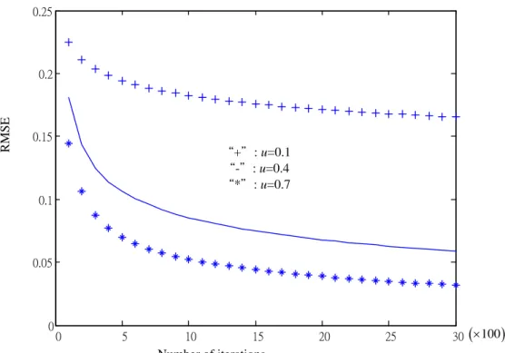
To examine the convergence characteristic of the proposed adaptive algorithm, we measure the RMSE performance with respect to the number of iterations and the results is presented in Fig. 2. Moreover, the simulations are performed using step size

µ =

0.1

, 0.4, and 0.7, respectively. As depicted in Fig. 2, RMSE decreases as n increases, which verifies the convergence characteristics. After about 1000 iterations, it converges to steady state. We can also observe from the figure that larger step size corresponds to faster speed of convergence.

The second simulation example aims to present the mismatch-induced performance degradation on the primary receiver. We fix the step size to be

µ =

0.1

, and exploit the number of iterations, n=500, 1000, and 2000 to stand for different extent of mismatch (estimation error). Fig. 3 evaluates the SINR (in dB) of arbitrary

PR with respect to 2 c

η







_σ







(in dB), which corresponds to the transmission power of CT. Since the primary users should not notice the existence of secondary users, we fix

2

p

η







_σ







to be 15 dB. The ideal case is also provided for measurement of SINR degradation. As shown in Fig. 3, SINR is intensely degraded for smaller n. This is as expected that the deviation of the estimated

{ }

_,

1, ,

cp k k= K

h

 from the true ones tends to be large under small n.

Specifically, we can observe from the figure that the SINR is very sensitive (severely degraded) according to 2 c

η







_σ







.

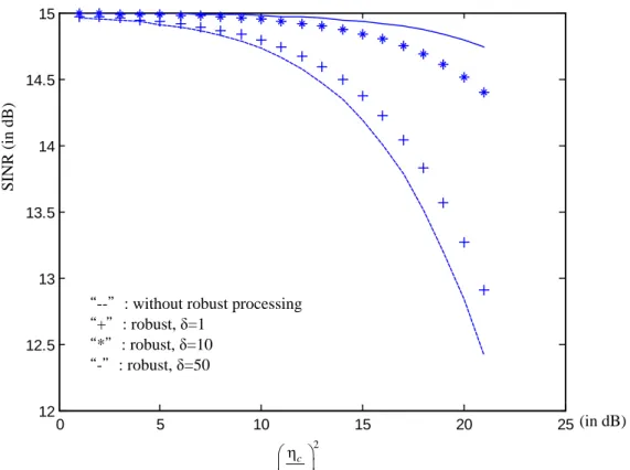
To examine the performance of the proposed robust null-steering scheme, we consider a mismatched scenario where

{ }

_, 1, , ˆ cp k k= K h

 arises from n=2000 iterations. By adding various diagonal loadings,

δ =

1, 10, 50, we evaluate the SINR performance of arbitrary PR with respect to

2

c

η







_σ







(in dB) and the result is presented in Fig. 4. Note that the case without robust processing is also provided for comparison. As demonstrated in Fig. 4, the SINR is enhanced by adding diagonal loading. In the final example, we examine the reliability of the proposed scheme. In the non-intrusive scheme,

η

2_c, which is up to our disposal, should be set within the region as deduced in (31) such that the SINRs at both PR and CR are above

γ

_th. Consequently, we may define the outage probability as

( )

(

)

2 2 2 2 2 ₁ 2 , 1

1

1

1

p p H H H outage th pc pc th H H cp k

P

P

− −





η







_

_η

_







σ









=

_

γ



_

+ >



_

−

_



γ



σ





















h P P P

P h

h



C C C

e

(39) In Fig. 5, we set 2

15

p

dB

η





=



_σ







, the threshold 2

10

th

_dB

γ



_{ =}



_σ







, and evaluate the outage probability with respect to the number of primary users (K), where each point is generated using 10,000 independent trials. We model the mismatch effect by generating

{ }

_,

1, ,

ˆ

cp k k= K

h

 using n=2000 iterations. As we can observe from the figure, the outage probability increases as K increases. Moreover, as array size increases (we use M=25, 40, 60, 80 for comparison), the outage probability is extensively reduced.

6. Conclusion

In this paper, we have proposed a non-intrusive cognitive system that employed adaptive nulls-steering techniques. Computer simulations confirm reliable convergent rate of the proposed RLS-gradient based iterative algorithm. In order to alleviate performance degradation induced by the mismatch effect, we have developed a robust processing scheme by adding diagonal loading. Compared with existing works related to the issue of robust beamforming in cognitive radio networks, the complexity is comprehensively reduced since the CSI is approximately known by the adaptive estimator. Simulation results demonstrated that the robust transmission beamforming scheme comprehensively outperform the SINR measured as mismatch occurs. Moreover, we have verified that the outage probability decreases to a large extent by adding the array size. Consequently, we can infer from the simulation results that the proposed non-intrusive cognitive scheme is suitable for practical use.

References

[1] S. Haykin, “Cognitive Radio: Brain-empowered wireless communications”, IEEE J. Selected Areas on

[2] D. Cabric, S. M. Mishra, and R. W. Brodersen, “Implementation issues in spectrum sensing for cognitive radios” in Proc. Asilomar Conf. Signals, System, Comput., vol.1, pp.772-776, Nov. 7-10, 2004.

[3] P. Kolodzy et al., “Next generation communications: Kickoff meeting” in Proc. DARPA, Oct. 17, 2001. [4] G. Ganesan, and Y. Li, “Cooperative spectrum sensing in cognitive radio networks”, IEEE Transaction on

Wireless Communications, vol. 6, pp.2204-2222, Jun. 2007.

[5] X. Liu and S. Shankar, “Sensing-based opportunistic channel access,” in ACM MONET, vol. 11, 2006. [6] D. Carbric, S. M. Mishra, D. Willkomm, R. Brodersen, and A. Wolisz, “A cognitive radio approach for usage

of virtual unlicensed spectrum,” in 14th IST Mobile and Wireless Communications Summit, 2005.

[7] E. Axell, G. Leus, E. G. Larsson and H. Vincent Poor, “Spectrum sensing for cognitive radio-State-of-the-art and recent advances”, IEEE Signal Processing Magazine, vol. 7, pp. 101-116, May 2012.

[8] K. B. Letaief and W. Zhang, “Cooperative communications for cognitive radio networks” Proceedings of the

IEEE, vol. 97, no. 5, pp. 878-893, May 2009.

[9] W. Zhang and K. B. Letaief, “Cooperative spectrum sensing with transmit and relay diversity in cognitive radio networks”, IEEE Transaction on Wireless Communications, vol. 7, pp.4761-4766, Dec. 2008.

[10] G. Kaur, P. P. Bhattacharya, “Cooperative spectrum sensing and spectrum sharing in cognitive radio: A review”, International Journal of Computer Applications in Engineering Sciences, vol. 1, issue 3, pp. 326-330, Sep. 2011.

[11] L. Shen, H. Wang, and W. Z. Zhao, “Blind spectrum sensing for cognitive radio channels with noise uncertainty”, IEEE Transaction on Wireless Communications, vol. 10, no. 6, pp. 1721–1724, 2011.

[12] S. Huang, Z. Ding, and X. Liu, “Non-Intrusive Cognitive Radio Networks based on Smart Antenna Technology” GLOBECOM 2007: 4862-4867.

[13] S. Haykin, Adaptive Filter Theory, 4th edition Prentice-Hall, Inc. 2002. [14] H. L. Van Trees, Optimum Array Processing, John Wiley & Sons, Inc., 2002.

[15] Z. Tian, K. L. Bell and H. L. Van Trees, “A recursive least squares implementation for LCMP beamforming under quadratic constraint”, IEEE Trans. Signal Processing, vol. 49, no. 6, pp. 1138-1145, June 2001.

Accept new data vector r(n) Update

( )

1 rr n − R Update Update Calculate c

w

Nonintrusive transmit beamforming by nulls-steering

(

)

{

hcp k, n+1

}

_k=1,,K

{ }

λk k=1,,K

“+”: u=0.1 “-”: u=0.4 “*”: u=0.7 0 5 10 15 20 25 30 0 0.05 0.1 0.15 0.2 0.25 RMSE Number of iterations

(

×100

)

Fig. 2: RMSE performance with respect to the number of iterations for

µ =

0.1

, 0.4, and 0.7, respectively.

0 5 10 15 20 25 8 9 10 11 12 13 14 15 (in dB) 2 c η    _σ    SINR (in dB ) “+”:ideal “--”: n=2000 “*”: n=1000 “-”: n=500

0 5 10 15 20 25 12 12.5 13 13.5 14 14.5 15 2 c η    _σ    (in dB) SINR (in dB )

“--”: without robust processing “+”: robust, δ=1

“*”: robust, δ=10 “-”: robust, δ=50

Fig. 4: SINR of primary receiver with respect to the SNR of cognitive transmitter with robust processing

3 4 5 6 7 8 9 10 11 12 0 0.1 0.2 0.3 0.4 0.5 0.6 0.7 0.8 0.9 Outage probability

Number of primary users “-”: M=25

“*”: M=40 “+”: M=60 “--”: M=80

認知型無線網路中之強健適應指向技術

武維疆

大葉大學電機系教授

wcwm53@mail.dyu.edu.tw

摘要 在本論文中我們提出了以智慧型天線技術為主應用於之認知型無線網路中之強健適應指向技術. 認 知型發射機 (CT), 配置天線陣列, 首先估計並追蹤與每個主要用戶間之通道向量. 接下來, CT 形成發射 波束並放置零點於主要用戶的方向上. 此外, 我們詳盡的分析估計誤差(不匹配)對於品質所造成的影響, 並證明了我們所提出的強健適應指向技術能有效的解決不匹配的問題. 電腦模擬的結果證明了我們所提 出的適應性演算法能有效的收斂. 除此之外, 我們也證明了只要有適當的天線數, 失效機率可保持非常的 低, 這也保證了我們所提出的架構之實用性. 關鍵字: 認知型無線電, 非侵入, 適應零點控制, 強健適應指向技術