發展與驗證虛擬網格切割模組於平行化直接模擬蒙地卡羅法程式

國 立 交 通 大 學

機

械

工

程

學

系

碩士論文

發展與驗證虛擬網格切割模組於平行化

直接模擬蒙地卡羅法程式

Development and Verification of a Virtual Mesh Refinement

Module in a Parallelized Direct Simulation Monte Carlo

Code (PDSC)

研 究 生：蘇正勤

指導教授：吳宗信 博士

發展與驗證虛擬網格切割模組於平行化

直接模擬蒙地卡羅法程式

Development and Verification of a Virtual Mesh Refinement

Module in a Parallelized Direct Simulation Monte Carlo

Code (PDSC)

研 究 生：蘇正勤

Student：Cheng-Chin Su

指導教授：吳宗信 博士 Advisor：Dr. Jong-Shinn Wu

國立交通大學

機械工程學系

碩 士 論 文

A Thesis

Submitted to Institute of Mechanical Engineering

College of Engineering

National Chiao Tung University

in Partial Fulfillment of the Requirements

for the Degree of

Master of Science

In

Mechanical Engineering

July 2008

Hisnchu, Taiwan

2008 年 7 月

誌謝

在交大兩年的求知路程，特別感謝指導教授吳宗信老師的照顧，讓我在學習過程及生 活方面都得到不少獲益。在研究及做學問方面，與老師的知識交流實令我感到獲益匪淺， 讓我能順利的踏入研究的領域並且不斷地成長。同時也感謝口試委員黃俊誠老師與江仲驊 老師在口試時提供的寶貴意見，使得本論文更加充實完備。另外特別感謝曾老大以及 Y 老 大不吝於付出時間與心力來教導我於研究中所遭遇的問題，以及粲哥、邱哥在研究上的啟 發和教導及生活上的鼓勵與幫助，在此一併致謝。 要感謝的人太多了，貴哥、徑全哥以及宗漢哥等已畢業的學長，以及實驗室的學長姐， 允民哥、周學姊、凱文兄、孟樺學姊、江學長。還有柳哥、育宗、阿龐、阿志、玟琪，與 你們努力奮鬥相處的時光應該是我最美好的回憶，還有穎志哥、古必等學弟妹們的協助， 使我這兩年過得相當充實且溫馨，並能順利完成學業。由於要感謝的人實在太多了，加上 篇幅有限，因此，在此一併致謝。 最後要特別感謝我的父母親以及家人，感謝他們對我的期許鼓勵及愛護，我會更加努 力朝向目標邁進。 蘇正勤 謹誌 2008 年 7 月于竹湖湖畔

發展與驗證虛擬網格切割模組於平行化直接模擬蒙地卡羅法程式

研究生: 蘇正勤 指導教授: 吳宗信 博士

國立交通大學

機械工程學系

摘要

本研究主要目的是發展與驗證虛擬網格切割模組(VMR)於平行化直接模擬摩地卡羅法 程式(PDSC)。在 DSMC 模擬中，網格被使用於分子的碰撞與巨觀性質的採樣，而網格的尺 寸必須小於局部平均自由路徑。然而，在模擬之前，並無法知道局部平均自由路徑的分佈。 在以前，我們研究室也曾經發展過數個網格切割法，使用 h-refinement 的方法於非結構性網 格中。然而，在被精細化的非結構性網格中，分子的追蹤是很困難的，而且網格的品質通 常很難保持。在本文中，我們將利用 transient adaptive sub-cells (TAS)的想法，發展出一個 新的非結構性網格切割法於 PDSC 中。這是一個二階虛擬網格切割法(two-level Virtual Mesh Refinement)。網格將在第一次 DSMC 模擬中被切割。被切割的網格稱做虛擬網格(virtual refined cells)，它們類似結構性網格。因此，分子的追蹤將變的有效率。這些虛擬網格被使 用於分子的碰撞與採樣。另外，我們使用蒙地卡羅積分法去計算每一個虛擬網格的面積。 5,000*Nvc 的 particles 數，對於每一個虛擬網格面積的計算可達到 0.1%的誤差，並且使用 12 個 CPU 計算 300,000 個虛擬網格面積所花的計算時間為 12.5 分鐘。僅有一個包含初始 網格質心的虛擬網格將被輸出作為初始網格的結果。這樣的一個方式將保持著記憶體使用

上的精簡，並且加上使用動態網格分解 (dynamic domain decomposition)去減少模擬所需要 的龐大時間。

最後，模擬兩個二維流場題目，包括極超音速流(M-12)流過一矩形物(argon gas, velocity=1413 m/s, temperature=40 K and Kn=0.05, number density=1.29E21 m-3)，以及極超音 速 流 (M-10) 流 過 一 圓 柱 物 (cylinder)(D=0.3048 m, argon gas, velocity=2634.1 m/s, temperature=200 K and Kn=0.0091, number density=4.274E20 m-3)，並且單獨使用四邊形、三 角形，以及四邊形與三角行的混合網格，進而去驗證程式的正確性。從這些模擬的結果顯 示，使用 VMR 不僅可以獲得 benchmark 的結果，而且也減少了三到四倍的計算時間。

Development and Verification of a Virtual Mesh Refinement Module in a

Parallelized Direct Simulation Monte Carlo Code (PDSC)

Student: Cheng-Chin Su Advisor: Dr. Jong-Shinn Wu

Department of Mechanical Engineering

National Chiao-Tung University

Abstract

The objective of this thesis is to develop and verify a virtual mesh refinement module (VMR), based on a new concept, in a parallelized direct simulation Monte Carlo code (PDSC). Cells are used for particle collisions and sampling of macroscopic properties in a DSMC simulation, in which the sizes have to be much smaller than the local mean free path. Unfortunately, it is generally impossible to know the distribution of local mean free path before the simulation. Previously, in our group we have developed several mesh refinement techniques in DSMC, which were based on the concept of h-refinement to unstructured grids. However, particle tracing on the refined unstructured mesh becomes inefficient and mesh quality is generally difficult to maintain. In this thesis, we will utilize the concept of transient adaptive sub-cells (TAS) proposed by Tseng et al. and propose a new type of mesh refinement on unstructured grids for DSMC simulation. This method is a two-level virtual mesh refinement, in which the background mesh is refined based on an initial DSMC simulation. The virtual refined cells are arranged in a way similar to the structured grid, which makes the particle tracing on them very efficient, unlike on unstructured grids. These virtual cells are used for particle collision and sampling. In addition, area of each virtual refined cell is calculated using the Monte Carlo integration method.

A

pproximately 5,000*Nvc particles are

required to reach 0.1% error for area calculations of all the

virtual refined

cells, which takes about 12.5 minutes of computational time for ~300,000 virtual refined cells using 12 processors. Only a virtual refined cell, which includes centroid of the background cell, we output only this data in each background cell. In this way, the original grid data structure is retained and memory cost is comparably low and using dynamic domain decomposition (DDD) to reduce computational time.

Finally, two two-dimensional test cases, which are Mach-12 hypersonic flow past a block (argon gas, velocity=1413 m/s, temperature=40 K and Kn=0.05, number density=1.29E21 m-3) and Mach-10 hypersonic flow past a circular cylinder (D=0.3048 m, argon gas, velocity=2634.1 m/s, temperature=200 K and Kn=0.0091, number density=4.274E20 m-3), including quadrilateral, triangular and mixed triangular-quadrilateral mesh have demonstrated in the thesis to show the robustness of this new mesh-refining algorithm. Results of cylinder simulation show that the case using VMR not only can faithfully reproduce the benchmark case, but also can reduce computational time from 15 hours (benchmark) to 3.5 hours (quadrilateral mesh), 4.5 hours (triangular mesh) and 5 hours (mixed quadrilateral-triangular mesh).

Table of Contents

誌謝 ...I 摘要 ... II Abstract...IV Table of Contents...VI List of Tables ... VIII List of Figures...IX Nomenclature... XIII

Chapter 1 Introduction... 1

1.1 Motivation and Background ... 1

1.1.1 Importance of Mesh Refinement ... 1

1.1.2 Classification of Flow Region ... 2

1.1.3 Direct Simulation Monte Carlo Method... 2

1.2 Literature Survey ... 3

1.3 Specific Objectives of the Thesis ... 4

Chapter 2 Numerical Methods... 5

2.1 The Boltzmann Equation ... 5

2.2 General Description of the standard DSMC... 6

2.3 General Description of the PDSC... 11

2.4 Transient Adaptive Sub-Cells in PDSC ... 13

2.5 Virtual Mesh Refinement Method ... 14

2.6 Dynamic Domain Decomposition ... 17

Chapter 3 Results and Discussion ... 18

3.1 Overview ...18

3.2 2-D Hypersonic Flow over a Block... 18

3.2.1 Problem Description and Simulated Condition ... 18

3.2.2 Verification of Virtual Mesh Refinement Method ... 19

3.2.2.1 Results of the Benchmark... 19

3.2.2.2 Compare Contours of Different Properties... 19

3.2.2.2.1 Density, Temperature and Velocity... 19

3.2.2.3 Properties along Different Profile... 20

3.2.2.4 Local Coefficient on Surface of the Block ... 20

3.3 2-D Hypersonic Flow over a Cylinder ... 20

3.3.1 Problem Description and Simulated Condition ... 20

3.3.2 Verification of Virtual Mesh Refinement Method ... 21

3.3.2.1 Results of the Benchmark... 21

3.3.2.2 Using Different Geometric Grids ... 21

3.3.2.3 Results of simulation with quadrilateral mesh ... 22

3.3.2.3.1 Compare Contours of Different Properties... 22

3.3.2.3.1.1 Density, Temperature and Velocity... 22

3.3.2.3.1.2 Collision Quality ... 22

3.3.2.3.2 Properties along Different Profile... 23

3.3.2.3.3 Surface Property on the Cylinder ... 23

3.3.2.4 Results of simulation with triangular mesh ... 23

3.3.2.4.1 Compare Contours of Different Properties... 23

3.3.2.4.1.1 Density, Temperature and Velocity... 23

3.3.2.4.1.2 Collision Quality ... 24

3.3.2.4.2 Properties along Different Profile... 24

3.3.2.4.3 Surface Property on the Cylinder ... 24

3.3.2.5 Results of simulation with mixed quadrilateral-triangular mesh... 25

3.3.2.5.1 Compare Contours of Different Properties... 25

3.3.2.5.1.1 Density, Temperature and Velocity... 25

3.3.2.5.1.2 Collision Quality ... 25

3.3.2.5.2 Properties along Different Profile... 25

3.3.2.5.3 Surface Property on the Cylinder ... 26

3.3.2.6 Comparison of Surface Properties with VMR on Different Geometric Grids ... 26

Chapter 4 Conclusions... 27

4.1 Summary... 27

4.2 Recommendation of Future Studies ... 27

List of Tables

Table I The simulation condition of the upstream for 2-D hypersonic flow over a block. ... 31 Table II The simulation condition of different cases for 2-D flow over a block. ... 32 Table III The simulation condition of the upstream for 2-D hypersonic flow over a cylinder. ... 33 Table IV The simulation condition of different cases with quadrilateral mesh for 2-D flow

over a cylinder. ... 34 Table V The simulation condition of different cases with triangular mesh for 2-D flow

over a cylinder. ... 35 Table VI The simulation condition of different cases with mixed quadrilateral-trianglar

List of Figures

Fig. 2.1 Classifications of Flow Region. ... 37

Fig. 2.2 The flowchart of the standard DSMC method. ... 38

Fig. 2.3 Simplified flow chart of the parallel DSMC method for np processors. ... 39

Fig. 2.4 The additional schemes in the parallel DSMC code. ... 40

Fig. 2.5 Division of structured and unstructured elements into sub-cells. ... 41

Fig. 2.6 The flowchart of DSMC simulation using virtual mesh refinement module... 42

Fig. 2.7 Division of structured and unstructured elements into refined cells... 43

Fig. 2.8 Distribution of random number in the refined background cell... 44

Fig. 2.9 Evolution of domain decomposition using 64 processors during the simulation: (a) initial; (b) intermediate; (c) final. ... 45

Fig. 3.1 Sketch of the computational domain of a argon hypersonic flow over a block (Ar gas, Kn∞=0.05,M∞=12, T∞=40 K, n∞=1.29E21 particles/m3) ... 46

Fig. 3.2 Computational domain of the benchmark (each cell size is 1/4 mean free path). .. 47

Fig. 3.3 Contours of computational results of the benchmark: (a) density; (b) temperature; (c) velocity in x-direction; (d) velocity in y-direction... 48

Fig. 3.4 Computation domain of VMR, TAS and None (each cell size is one mean free path). ... 49

Fig. 3.5 Compared contour of density of the benchmark, VMR, TAS and None. ... 50

Fig. 3.6 Compared contour of temperature of the benchmark, VMR, TAS and None... 51

Fig. 3.7 Compared contour of u-velocity of the benchmark, VMR, TAS and None... 52

Fig. 3.8 Compared contour of v-velocity of the benchmark, VMR, TAS and None... 53

Fig. 3.9 Contour of mcs/mpfs: (a) benchmark; (b) VMR; (c) TAS; (d) None. ... 54

Fig. 3.10 Profile of the benchmark, VMR, TAS, and None along x=0.01 m: (a) density; (b) temperature; (c) u-velocity; (d) v-velocity... 55

Fig. 3.11 Profile of the benchmark, VMR, TAS, and None along x=0.005 m: (a) density; (b) temperature; (c) u-velocity; (d) v-velocity... 56

Fig. 3.12 Profile of the benchmark, VMR, TAS, and None along x=0.0005 m: (a) density; (b) temperature; (c) u-velocity; (d) v-velocity. ... 57

Fig. 3.13 Profile of the benchmark, VMR, TAS, and None along y=0.02 m: (a) density; (b) temperature; (c) u-velocity; (d) v-velocity... 58

Fig. 3.14 Compared local pressure coefficient along x=0 m on block... 59

Fig. 3.15 Compared local friction coefficient along x=0 m on block. ... 60

Fig. 3.16 Compared local pressure coefficient along y=0.01 m on block... 61

Fig. 3.17 Compared local friction coefficient along y=0.01 m on block. ... 62

Fig. 3.18 Sketch of the computational domain of a argon hypersonic flow over a cylinder (Ar gas, Kn∞=0.0091, M∞=10, T∞=200 K, n∞=4.274E20, particles/m3)... 63

Fig. 3.19 Computational domain of the benchmark. ... 64

Fig. 3.20 Contours of computational results of the benchmark: (a) density; (b) temperature; (c) velocity in x-direction; (d) velocity in y-direction... 65

Fig. 3.21 Using quadrilateral computation domain of VMR, TAS and None. ...66

Fig. 3.22 Compared contour of density of the benchmark, VMR, TAS and None with quadrilateral mesh. ... 67

Fig. 3.23 Compared contour of temperature of the benchmark, VMR, TAS and None with quadrilateral mesh. ... 68

Fig. 3.24 Compared contour of u-velocity of the benchmark, VMR, TAS and None with quadrilateral mesh. ... 69

Fig. 3.25 Compared contour of v-velocity of the benchmark, VMR, TAS and None with quadrilateral mesh. ... 70

Fig. 3.26 Contour of mcs/mpfs with quadrilateral mesh: (a) benchmark; (b) VMR; (c) TAS; (d) None... 71

Fig. 3.27 Profile of the benchmark, VMR, TAS, and None along x=0.005 m with quadrilateral mesh: (a) density; (b) temperature; (c) u-velocity; (d) v-velocity. ... 72

Fig. 3.28 Profile of the benchmark, VMR, TAS, and None along x=0.4 m with quadrilateral mesh: (a) density; (b) temperature; (c) u-velocity; (d) v-velocity. ... 73

Fig. 3.29 Profile of the benchmark, VMR, TAS, and None along x=0.5 m with quadrilateral mesh: (a) density; (b) temperature; (c) u-velocity; (d) v-velocity. ... 74

Fig. 3.30 Profile of the benchmark, VMR, TAS, and None along y=0.2 m with quadrilateral mesh: (a) density; (b) temperature; (c) u-velocity; (d) v-velocity. ... 75

Fig. 3.31 Compared local coefficient along surface of cylinder with quadrilateral mesh: (a) pressure coefficient; (b) friction coefficient; (c) heat transfer coefficient... 76

Fig. 3.32 Using triangular computation domain of VMR, TAS and None... 77

Fig. 3.33 Compared contour of density of the benchmark, VMR, TAS and None with triangular mesh. ...78 Fig. 3.34 Compared contour of temperature of the benchmark, VMR, TAS and None with

triangular mesh. ... 79 Fig. 3.35 Compared contour of u-velocity of the benchmark, VMR, TAS and None with

triangular mesh. ... 80 Fig. 3.36 Compared contour of v-velocity of the benchmark, VMR, TAS and None with

triangular mesh. ... 81 Fig. 3.37 Contour of mcs/mpfs with triangular mesh: (a) benchmark; (b) VMR; (c) TAS; (d)

None. ... 82 Fig. 3.38 Profile of the benchmark, VMR, TAS, and None along x=0.005 m with triangular

mesh: (a) density; (b) temperature; (c) u-velocity; (d) v-velocity. ... 83 Fig. 3.39 Profile of the benchmark, VMR, TAS, and None along x=0.4 m with triangular

mesh: (a) density; (b) temperature; (c) u-velocity; (d) v-velocity. ... 84 Fig. 3.40 Profile of the benchmark, VMR, TAS, and None along x=0.5 m with triangular

mesh: (a) density; (b) temperature; (c) u-velocity; (d) v-velocity. ... 85 Fig. 3.41 Profile of the benchmark, VMR, TAS, and None along y=0.2 m with triangular

mesh: (a) density; (b) temperature; (c) u-velocity; (d) v-velocity. ... 86 Fig. 3.42 Compared local coefficient along surface of cylinder with triangular mesh: (a)

pressure coefficient; (b) friction coefficient; (c) heat transfer coefficient... 87 Fig. 3.43 Using mixed quadrilateral-triangular computation domain of VMR, TAS and

None. ... 88 Fig. 3.44 Compared contour of density of the benchmark, VMR, TAS and None with

mixed quadrilateral-triangular mesh... 89 Fig. 3.45 Compared contour of temperature of the benchmark, VMR, TAS and None with

mixed quadrilateral-triangular mesh... 90 Fig. 3.46 Compared contour of u-velocity of the benchmark, VMR, TAS and None with

mixed quadrilateral-triangular mesh... 91 Fig. 3.47 Compared contour of v-velocity of the benchmark, VMR, TAS and None with

mixed quadrilateral-triangular mesh... 92 Fig. 3.48 Contour of mcs/mpfs with mixed quadrilateral-triangular mesh: (a) benchmark; (b)

VMR; (c) TAS; (d) None. ... 93 Fig. 3.49 Profile of the benchmark, VMR, TAS, and None along x=0.005 m with mixed

quadrilateral-triangular mesh: (a) density; (b) temperature; (c) u-velocity; (d) v-velocity. ... 94 Fig. 3.50 Profile of the benchmark, VMR, TAS, and None along x=0.4 m with mixed

v-velocity. ... 95 Fig. 3.51 Profile of the benchmark, VMR, TAS, and None along x=0.5 m with mixed

quadrilateral-triangular mesh: (a) density; (b) temperature; (c) u-velocity; (d) v-velocity. ... 96 Fig. 3.52 Profile of the benchmark, VMR, TAS, and None along y=0.2 m with mixed

quadrilateral-triangular mesh: (a) density; (b) temperature; (c) u-velocity; (d) v-velocity. ... 97 Fig. 3.53 Compared local coefficient along surface of cylinder with mixed

quadrilateral-triangular mesh: (a) pressure coefficient; (b) friction coefficient; (c) heat transfer coefficient. ... 98 Fig. 3.54 Compared local coefficient along surface of cylinder with different grids, include

quadrilateral, triangular and mixed quadrilateral-triangular grids: (a) pressure coefficient; (b) friction coefficient; (c) heat transfer coefficient. ... 99

Nomenclature

λ ：mean free path

ρ ：density

σ ：the differential cross section ω ：viscosity temperature exponent Ω : space domain rot ε ：rotational energy v ε ：vibrational energy rot

ζ ：rotational degree of freedom

v

ζ ：vibrational degree of freedom Ut ：time-step

σT ：the total cross section

c ：the total velocity

c’ ：random velocity

co ：mean velocity

cr ：relative speed

d ：molecular diameter

dref ：reference diameter

dcen ：the distance between center of the virtual cell and background cell

E ：energy

Kn ：Knudsen number

Knmax : continuum breakdown parameter

. max Thr

Kn : the threshold value of continuum breakdown parameter

Q

Kn _{: local Knudsen numbers based on flow property Q}

L ：characteristic length

m ：molecule mass

n ：number density

Tne

P : thermal non-equilibrium indicator

. Thr Tne

P : the threshold value of thermal non-equilibrium indicator

Re ：Reynolds number

T∞ ：free-stream temperature

Tref ：reference temperature

Trot ：rotational temperature

Ttot ：total temperature

Ttr ：translational temperature

Tv ：vibrational temperature

Chapter 1 Introduction

1.1 Motivation and Background

1.1.1 Importance of Mesh Refinement

The mesh refinement scheme is very important problem for numerical method. The Direct Simulation Monte Carlo (DSMC) method is a computational tool for the simulation of flows in which effects at the molecular scale become significant [5]. Cells are used for particle collisions and sampling of macroscopic properties in a DSMC simulation, in which the sizes have to be much smaller than the local mean free path. Unfortunately, it is generally impossible to know the distribution of local mean free path before the simulation. In order to obtain better resolution of space and physics, we develop and verify a new mesh refinement module, based on a new concept, in a parallelized direct simulation Monte Carlo code (PDSC). In the past, we had develop had developed two- and three-dimensional adaptive mesh refinement modules for triangular- and tetrahedral cells, respectively [24, 25], based on the concept of h-refinement similar to those employed in computational fluid dynamics. However, particle tracing on the refined unstructured mesh becomes inefficient and mesh quality is generally difficult to maintain. In this thesis, we will utilize the concept of transient adaptive sub-cells (TAS) proposed by Tseng et al. [18] and propose a new type of mesh refinement on unstructured grids for DSMC simulation. This method is a two-level virtual mesh refinement, in which the background mesh is refined based on an initial DSMC simulation. Finally, several 2D test cases including triangular, quadrilateral and mixed triangular-quadrilateral mesh will be demonstrated in the thesis to show the robustness of this new mesh-refining algorithm.

1.1.2 Classification of Flow Region

Knudsen number (Kn=λ/L) is usually used to indicate the degree of rarefaction. The mean free path λ is the average distance traveled by molecules before collision and L is the flow characteristic length. In general, flow are divided into four regimes and three solutions. When the local Knudsen number approaches zero, the flow reaches inviscid limit and can be solved by Euler equation. When the flow is close to the continuum regime (Kn approach 0.01), the well known Navier-Stokes equation may be applied to obtain accurate result for engineering purposes. When Kn is the larger than 0.01, assumption of continuum begins to break down and the particle-based method is necessary and a kinetic approach, based on the Boltzmann equation [7]. It is important to note that the kinetic approach is valid in the whole range of the gas rarefaction. However, it is rarely used to numerically solve the practical problems because of two major difficulties. They are included higher dimensionality (up to seven) of the Boltzmann equation and the difficulties of correctly modeling the integral collision term. The well known direct simulation Monte Carlo (DSMC) method [5] is also a powerful computational scheme.

1.1.3 Direct Simulation Monte Carlo Method

Direct Simulation Monte Carlo (DSMC), was proposed by Bird to solve the Boltzmann equation using direct simulation of particle collision kinetics, and the associated monograph was published in 1994 [5]. Later on, both Nanbu [14] and Wagner [19] were able to demonstrate mathematically that the DSMC method is equivalent to solving the Boltzmann equation as the simulated number of particles become large. The DSMC method is a particle-based method for the simulation of flow of gas. The gas is modeled at the microscopic level using simulated particles, which each represents a large number of physical molecules or atoms. And gas dynamics are modeled through between the motion of particles

and collisions. The mass, momentum and energy transports between particles are considered at the particle level. The method is statistical in nature and depends heavily upon pseudo-random number sequences for simulation. Physical events such as collisions are handled probabilistically using largely phenomenological models, which are designed to reproduce real fluid behavior when examined at the macroscopic level. This method had been widely used computational tool for the simulation of flow of gas in the rarefied regime, in which molecular effects become important.

1.2 Literature Survey

Mesh criterion is an important factor to the DSMC simulation [5] because the domain is discreted into mesh for particle movements and collisions. Several mesh refinement algorithms are proposed to conquer the mesh issue, including h-refinement, re-mesh and moving mesh. In the past, we had developed two- and three-dimensional adaptive mesh refinement modules for triangular- and tetrahedral cells, respectively [24, 25], based on the concept of h-refinement similar to those employed in computational fluid dynamics. Several inherent problems arise, which include: 1) Refined cell becomes skewed due to hanging-node removal, which makes particle tracking more difficult; 2) Particles are tracked on refined unstructured grids, which is slow as compared to structured grids; 3) Hanging-node removal algorithm becomes very complicated, especially, in three-dimensional case [24]; 4) Difficult to parallelize due to complicated data structure [24]; and 5) Increasing memory as compared to the original gird. Thus, an alternative algorithm of mesh refinement on unstructured grids, which is free of the above problems, is critical in applying unstructured grids in the parallel DSMC method [25].

At present, Tseng et al. [18] had proposed a sub-cell module that named transient adaptive sub-cell (TAS) module to ensure to obtain the better collision behavior. A new

module with same idea is proposed to virtually refine cells, which is named two-level virtual mesh refinement (VMR) algorithm. This proposed module uses the virtual cells for particles collision and sampling. It is supposed can obtain accurate results without scarifying the memory cost h-refinement method and difficult to particle tracing.

1.3 Specific Objectives of the Thesis

The current objectives of this thesis are summarized as follows:

1. To develop and verify the virtual mesh refinement module for a Parallel DSCM code on unstructured grids.

2. To simulate 2-D hypersonic flow over a block with different size of cells, including Mach number=12 argon of the upstream speed, temperature T_∞ = 4 0K and density

ρ_∞ = 8.6043E-5 3

kg/m .

3. To simulate 2-D hypersonic flow over a cylinder with different size of cells, including Mach number=10 argon of the upstream speed, temperature T_∞ = 2 0 0 K and density

ρ_∞ = 2.8327E-5 3

kg/m .

4. To verify and discuss the effects of virtual mesh refinement module in PDSC.

The organization of the thesis is stated as follows: Chapter 1 describes the Introduction, Chapter 2 describes the Numerical Method, Chapter 3 describes the verification of virtual mesh refinement module, and followed by the Results and Discussion. Finally Chapter 4 describes the Conclusions.

Chapter 2 Numerical Methods

2.1 The Boltzmann Equation

The Knudsen number (Kn) is used to indicate the degree of rarefaction. In Fig. 2.1 [5], flows are divided into four regimes and three solutions. We have found the Boltzmann equation is valid for all flow regimes. It is one of the most important transport equations in non-equilibrium statistical mechanics, which deals with systems far from thermodynamics equilibrium. There are some assumptions made in the derivation of the Boltzmann equation which defines limits of applicability. They are summarized as follows:

1. Molecular chaos is assumed which is valid when the intermolecular forces are short range. It allows the representation of the two particles distribution function as a product of the two single particle distribution functions.

2. Distribution functions do not change before particle collision. This implies that the encounter is of short time duration in comparison to the mean free collision time. 3. All collisions are binary collisions.

4. Particles are uninfluenced by intermolecular potentials external to an interaction. According to these assumptions, the Boltzmann equation is derived and shown as

4 2 ' ' 1 1 0 ( ) ( ) ( ) ( ) i i c i i i nf nf nf f u F n f f ff g d dU t x u x π σ ∞ −∞ ∂ ∂ ∂ ∂ + + = = − Ω ∂ ∂ ∂ ∂

∫ ∫

(2.1)

Meaning of particle phase-space distribution function f is the number of particles

with center of mass located within a small volume d r near the point r , and velocity within 3

a ranged u , at time t . 3 F is an external force per unit mass and t is the time and _i u is the _i

molecular velocity. σ is the differential cross section and dΩ is an element of solid angle. The prime denotes the post-collision quantities and the subscript 1 denotes the collision

partner. Meaning of each term in Eq. (2.1) is described in the following;

1. The first term on the left hand side of the equation represents the time variation of the distribution function of the particles (unsteady term).

2. The second term gives the spatial variation of the distribution function (flux term). 3. The third term describes the effect of a force on the particles (force term).

4. The term at right hand side of the equation is called the collision integral (collision term). It is the source of most of the difficulties in obtaining solutions of the Boltzmann equation.

In general, it is difficult to solve the Boltzmann equation directly using numerical method because the difficulties of correctly modeling the integral collision term. Instead, the DSMC method was used to simulated problems involving rarefied gas dynamics, which is the main topic in the current thesis.

2.2 General Description of the standard DSMC

In order to the expected rarefaction caused by the rarefied gas flows, the direct simulation Monte Carlo (DSMC) method which is a particle-based method developed by Bird during the 1960s and it is widely used an efficient technique to simulate rarefied gas regime [2, 5]. In the DSMC method, a large number of particles are generated in the flow field to represent real physical molecules rather than a mathematical foundation and it has been proved that the DSMC method is equivalent to solving the Boltzmann equation [14, 19]. The assumptions of molecular chaos and a dilute gas are required by both the Boltzmann formulation and the DSMC method [2, 5]. An important feature of DSMC is that the molecular motion and the intermolecular collisions are uncoupled over the time intervals that are much smaller than the mean collision time. Both the collision between molecules and the interaction between molecules and solid boundaries are computed on a probabilistic basis and,

hence, this method makes extensive random numbers. In most practical applications, the number of simulated molecules is extremely small compared with the number of real molecules. The general procedures of the DSMC method are described in the next section, and the consequences of the computational approximations can be found in Bird [2, 5].

In DSMC, there are three molecular collision models for real physical behavior and imitate the real particle collision, which are the Hard Sphere (HS), Variable Hard Sphere (VHS) and Variable Soft Sphere (VSS) molecular models, in the standard DSMC method [5]. The collision pairs are chosen by the acceptance-rejection method. The no time counter (NTC) method is an efficient method for molecular collision. This method yield the exact collision rate in both simple gases and gas mixtures, and under either equilibrium or non-equilibrium conditions.

Fig. 2.2 is a general flowchart of the standard DSMC method. Important steps of the DSMC method include setting up the initial conditions, moving all the simulated particles, indexing all the particles, colliding between particles and sampling the molecules within cells to obtain the macroscopic quantities. The details of each step will be described in the following:

z Initialization

The first step to use the DSMC method in simulating flows is to set up the geometry and flow conditions. A physical space is discredited into a network of cells and the domain boundaries have to be assigned according to the flow conditions. An important feature has to be noted is the size of the computational cell should be smaller than the mean free path, and the distance of the molecular movement per time step should be smaller than the cell dimension. After the data of geometry and flow conditions have been read in the code, the numbers of each cell is calculated according to the free-stream number density and the current cell volume. The initial particle velocities are assigned to each particle based on the

Maxwell-Boltzmann distribution according to the free-stream velocities and temperature, and the positions of each particle are randomly allocated within the cells.

z Particle Movement

After initialization process, the molecules begin move one by one, and the molecules move in a straight line over the time step if it did not collide with solid surface. For the standard DSMC code by Bird [2, 5], the particles are moved in a structured mesh. There are two possible conditions of the particle movement. First is the particle movement without interacting with solid wall. The particle location can be easy located according to the velocity and initial locations of the particle. Second is the case that the particle collides with solid boundary. The velocity of the particle is determined by the boundary type. Then, the particle continues its journey from the intersection point on the cell surface with its new absolute velocity until it stops. Although it is easier to implement by using structured mesh, it is difficult for those flows with complex geometry.

z Indexing

The location of the particle after movement with respect to the cell is important information for particle collisions. The relations between particles and cells are reordered according to the order of the number of particles and cells. Before the collision process, the collision partner will be chosen by a random method in the current cell. And the number of the collision partner can be easy determined according to this numbering system.

z Gas-Phase Collisions

The other most important phase of the DSMC method is gas phase collision. The current DSMC method uses the no time counter (NTC) method to determine the correct collision rate in the collision cells. The number of collision pairs within volume (area) of the cell V over a time interval _C Δt is calculated by the following equation;

1 ( )_max /

Where N and N are fluctuating and average number of simulated particles, respectively.

N

F is the particle weight, which is the number of real particles that a simulated particle

represents. σ_T and c are the cross section and the relative speed, respectively. The _r collision for each pair is computed with probability

(σ_Tc_r)/(σ_Tc_r)_max (2.3) The collision is accepted if the above value for the pair is greater than a random fraction. Each cell is treated independently and the collision partners for interactions are chosen at random, regardless of their positions within the cells. The collision process is described sequentially as follows:

1. The number of collision pairs is calculated according to the NTC method, Eq. (2.2), for each cell.

2. The first particle is chosen randomly from the list of particles within a collision cell.

3. The other collision partner is also chosen at random within the same cell.

4. The collision is accepted if the computed probability, Eq. (2.3), is greater than a random number.

5. If the collision pair is accepted then the post-collision velocities are calculated using the mechanics of elastic collision. If the collision pair is not to collide, continue choosing the next collision pair.

6. If the collision pair is polyatomic gas, the translational and internal energy can be redistributed by the Larsen and Borgnakke model [6], which assumes in equilibrium.

z Sampling

After the particle movement and collision process finish, the particle has updated positions and velocities. The macroscopic flow properties in each cell are assumed to be constant over the cell volume and are sampled from the microscopic properties of each particle within the cell. The macroscopic properties, including density, velocities and temperatures, are calculated in the following equations [2, 5];

nm = ρ _(2.4a) ' c c c c_o = = _o + (2.4b) ) ' ' ' ( 2 1 2 3 2 2 2 w v u m kT_tr = + + (2.4c) ) ( 2 r rot rot k T = ε ζ (2.4d) ) ( 2 v v v k T = ε ζ (2.4e) ) 3 ( ) 3

( _{tr rot rot v v rot v}

tot T T T

T = +ζ +ζ +ζ +ζ (2.4f)

Where n, m are the number density and molecule mass, receptively. c, co, and c’ are the total

velocity, mean velocity, and random velocity, respectively. In addition, Ttr, Trot, Tv and Ttot are

translational, rotational, vibration and total temperature, respectively. ε_rot andε_vare the rotational and vibration energy, respectively. ζrot and ζv are the number of degree of

freedom of rotation and vibration, respectively.

If the simulated particle is monatomic gas, the translational temperature is regarded simply as total temperature. Vibration effect can be neglect if the temperature of the flow is low enough.

The flow will be monitored if steady state is reached. If the flow is under unsteady situation, the sampling of the properties should be reset until the flow reaches steady state. As a rule of thumb, the sampling of particles starts when the number of molecules in the

calculation domain becomes approximately constant.

2.3 General Description of the PDSC

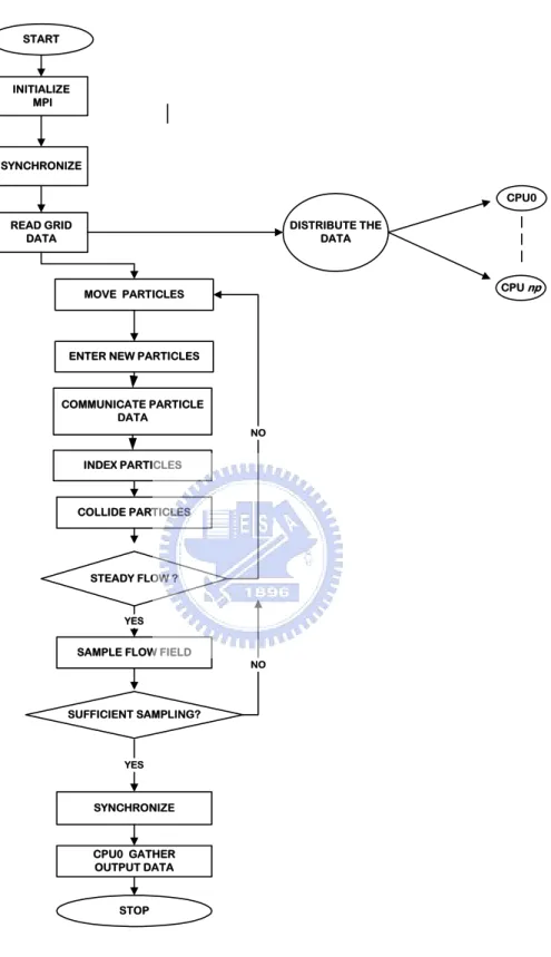
Although the large number of particles in a real gas is replaced with a reduced number of particles, there are still a large number of particles must be simulated, leading to tremendous computer power requirements and needing to cost a lot of computational time. As a result, parallel DSMC method is developed to solve the problem. Fig. 2.3 illustrates a simplified flow chart of the parallel DSMC method used in the current research. The DSMC algorithm is readily parallelized through physical domain decomposition. The cells of the computational grid are distributed each the processors. Each processor executes the DSMC algorithm in serial for all particles and cells in its domain. The data communication occurs when particles cross the domain (processor) boundaries and transferred between processors.

Parallel DSMC Code (PDSC) is the main solver used in this thesis, which utilizes unstructured tetrahedral mesh. Fig. 2.4 is the features of PDSC and brief introduction is listed in the following paragraphs.

1. 2D/2D-axisymmetric/3-D unstructured-grid topology: PDSC can accept either

2D/2D-axisymmetric (triangular, quadrilateral or hybrid triangular-quadrilateral) or 3D (tetrahedral, hexahedral or hybrid tetrahedral-hexahedral) mesh [25]. Computational cost of particle tracking for the unstructured mesh is generally higher than that for the structured mesh. However, the use of the unstructured mesh, which provides excellent flexibility of handling boundary conditions with complicated geometry and of parallel computing using dynamic domain decomposition based on load balancing, is highly justified.

multi-level graph-partitioning tool, PMETIS [21] by taking advantage of the unstructured mesh topology employed in the code. A decision policy for repartition with a concept of Stop-At-Rise (SAR) [21] or constant period of time (fixed number of time steps) can be used to decide when to repartition the domain. Capability of repartitioning of the domain at constant or variable time interval is also provided in PDSC. Resulting parallel performance is excellent if the problem size is comparably large. Details can be found in Wu and Tseng [21].

3. Spatial variable time-step scheme: PDSC employs a spatial variable time-step

scheme (or equivalently a variable cell-weighting scheme), based on particle flux (mass, momentum, energy) conservation when particles pass interface between cells. This strategy can greatly reduce both the number of iterations towards the steady state, and the required number of simulated particles for an acceptable statistical uncertainty. Past experience shows this scheme is very effective when coupled with an adaptive mesh refinement technique [24].

4. Unsteady flow simulation: An unsteady sampling routine is implemented in PDSC,

allowing the simulation of time-dependent flow problems in the near continuum range [9]. A post-processing procedure called DSMC Rapid Ensemble Averaging Method (DREAM) is developed to improve the statistical scatter in the results while minimizing both memory and simulation time. In addition, a temporal variable time-step (TVTS) scheme is also developed to speed up the unsteady flow simulation using PDSC. More details can be found in [9].

5. Transient Sub-cells: Recently, transient sub-cells are implemented in PDSC directly

on the unstructured grid, in which the nearest-neighbor collision can be enforced, whilst maintaining minimal computational overhead [18]. Details of the idea and implementation are described next.

2.4 Transient Adaptive Sub-Cells in PDSC

The implementation of transient adaptive sub-cells (TAS) in PDSC allows to obtain the better collision quality for the same grid, even for grids which are “under-resolved”. Running simulations with under-resolved sampling cells which employ sub-cells results in a reduction in the computational and memory requirements of the simulation, albeit at the cost of a reduction in the possible sampling resolution of the macroscopic properties, but without sacrificing simulation accuracy.

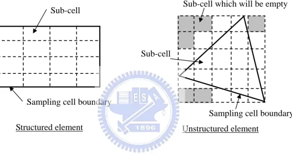
In PDSC, unstructured grids are used, requiring an adaptation of the transient adaptive sub-cells scheme, which was originally promoted by Bird [DS2V code by Bird]. In PDSC, the sampling cells are divided into sub-cells during the collision routine. Because the sub-cells only exist in one sampling cell at a time, and only during the collision routine, they can be considered “transient adaptive sub-cells” which will have negligible computer memory overhead. In every case, these sub-cells are quadrilateral in 2D or hexahedral in 3D which reduces the complexity of sub-dividing the sampling cell and greatly facilitates particle indexing. The size of the sub-cells is indirectly controlled by the user, who inputs the desired averaged number of particles per sub-cell, P. The dimensions of the sub-cell array for program based on the number of particles in the background cell, Nparts. Briefly, the total

number of sub-cells are computed by the rule for the 2-D case

parts parts

N N

P × P _(2.5) Fig. 2.5 shows the way in which both rectangular and triangular sampling background

cells are divided into sub-cells. As can be seen, in the unstructured case, there may be sub-cells which are entirely outside the boundary of the sampling cell, however this has no affect on the collision routine. In both cases, the concept is easily extended to three-dimensional sampling cells.

During the collision routine, a particle is chosen at random within the whole sampling cell. The sub-cell in which the particle lies is then determined and if another particle is in the same sub-cell then these particles are chosen for collision. If the first particle is alone within the sub-cell, then adjacent sub-cells are scanned for a collision partner. These sub-cell routines ensure nearest neighbor collisions, even within under-resolved sampling cells, with minimal computational and memory overhead.

Bird has also shown that preventing particles from colliding again their last collision partner, reduces the error in some variables such as heat transfer and shear stress by up to 5% [ref-Bird manual of DS2V code]. The basis of this is that collisions between particles which just collided with each other is unphysical, since the particle must be moving away from each other after the first collision. A minor modification was made to PDSC to prevent particles colliding with their last collision partner. This involved the creation of an array in which the last collision partner for every particle is stored and if the two particles are subsequently chosen for collision without having collided with any other particle, the collision is rejected.

2.5 Virtual Mesh Refinement Method

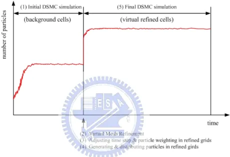
In DSMC, the cells are used to collision and sampling. In general, the size of each cell has been 1/2-1/3 local mean free path. But it is difficult. In this thesis, we will base on TAS scheme to develop a new module for PDSC. It named Virtual Mesh Refinement (VMR). Fig. 2.6 shows the temporal evolution of the DSMC method with the VMR module, which is described next. These steps include: 1) The initial DSMC simulation on the background grids, 2) Virtual mesh refinement based on the data obtained in Step 1), 3) Adjusting the time step size and particle weighting in the refined cells accordingly, 4) Generating and randomly distributing particles in the refined cells based on Maxwellian distribution of velocities, and 5) Final DSMC simulation on the refined grids. Note TAS

function is used throughout the whole procedures to ensure the good collision quality. Some of the details in the above procedures are described in the following.

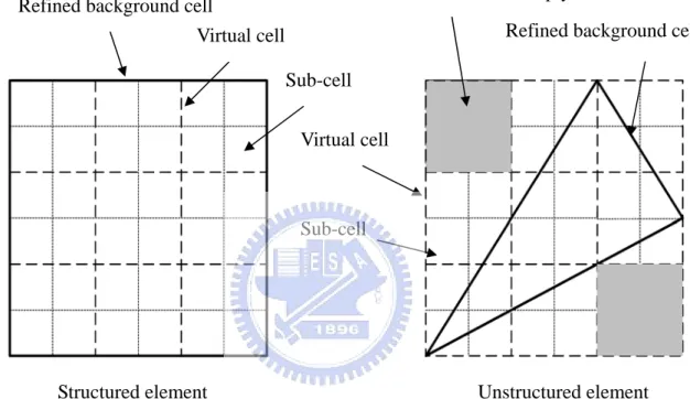
The refinement happens when the square root of background cell area satisfies

bc local

A ≥λ ⋅ (2.6) α where A , _bc λ_local and α are background cell area, local mean free path and a factor adjust by user to control the refined mesh quality, respectively. The virtual cells spacing is based on 1/2 local mean free path in the refined background cell. Fig. 2.7 is shown relationship between the refined background cell and virtual cells, include quadrilateral and triangular grid. In addition to refine background cells, the VMR module is adjusting time step and particle weighting for each refined background cell and generating new particles based on local velocity and temperature in the refined background cells. The adjusting of time step is written as adjust vc

t

t

N

Δ

Δ

=

(2.7) where Δt_adjust and N are adjusting of time step and number of virtual cell in the refined _vc background cell, respectively. The adjusting of particle weighting is written as

adjust N N vc

F

F

N

=

_(2.8) where adjust N

F

is adjusting of particle weighting. Afterward reset all sampling data and begin second transient period.

Firstly, particle movement based on new adjusted time step in the refined background cells. Then gas phase collision is as based on adjusted time step, weighting and area (volume) of the virtual cell to determine the correct number of collision pair in the virtual cells. Therefore, Eq. 2.2 becomes as

1 ( )_max /

2N NFNadjust σTcr Δtadjust Vvc (2.9)

where V is area (volume) of the virtual cell. _vc

The area of virtual cells calculating algorithm of two-dimensional unstructured grids is complicated, especially, and cannot practically use in the three-dimensional case in the future. One of the easy ways to get the area of the virtual cell is by means of Monte Carlo integration method. The sufficient random number of 5000×Nvc in the refined background cell is used

in the area integration, which the error is about 0.1% in each virtual cell. The total area calculation time is about 12.5 minutes in parallel program, in which the number of virtual cell, for example, is 300,000, and CPU number is 12. Fig. 2.8 shows distribution of random number in the refined background cell and virtual cell. We calculate total random number for each virtual cell. Therefore, the area (volume) of the virtual cell is calculated by the following equation; 1 i vc i vc c N i i R V V R = = ×

∑

(2.10) Where subscript i , R and

1 vc N i i R =

∑

are index of virtual cell number from 1 to N , total _vc random number in i th virtual cell and sufficient random number 5000×N_vc in the refined background cell, respectively. See Fig. 2.7, gas phase collision is shown to using transient adaptive sub-cell method within virtual cells to select collided particles.

During final sampling period, the microscopic properties are sampled in the virtual cells. Finally, only a virtual cell, which includes the centroid of the refined background cell, is output in the refined background cell. In this way, the original grid data structure is retained and memory cost is comparably low.

2.6 Dynamic Domain Decomposition

In PDSC, we had developed dynamic domain decomposition scheme [21] to reduce computational time. In here, we have applied this to VMR module. In Fig. 2.9 (a), it is showing partition domain to different CPU before simulation by 64 processors. Fig. 2.8(b) shows repartition domain to different CPU during simulation. Finally, Fig. 2.9 (c) shows repartition domain after simulation. In this way, repartition domain is based on particle number in each CPU to balance computational loading of each CPU to reduce simulation time.

Chapter 3 Results and Discussion

3.1 Overview

In this thesis, we were simulated two major cases. One of these is two-dimensional hypersonic flow over a block (M=8). Other case is two-dimensional hypersonic flow over a cylinder (M=10) using different geometric grids. As fluid flow over a block/cylinder, to result bow shock. Then, density in the flow field is to increase and to cause that initial cells size are the bigger than local mean free path. Therefore, we have used fewer cells than simulation of benchmark, to verify that the results using virtual mesh refinement module in PDSC are still to keep level of benchmark solution.

3.2 2-D Hypersonic Flow over a Block

3.2.1 Problem Description and Simulated Condition

The condition for this simulation with Mach number 12 Argon is shown in Fig. 3.1. The upstream velocity, temperature and number density is equal to 1413 m/s, 40 K and 1.29E+21 particles/ 3

m , respectively. Although this problem is a two-dimensional case, will be simulated four cases with the different cell size. First, the grid of benchmark spacing was chosen to be 1/4 the mean free path based on simulation condition of free stream. Second, the grid spacing of other cases was chosen to be one the mean free path. In these cases, we will use different module for simulation of PDSC, including VMR, TAS module and None. The simulation condition of these cases is shown in Table I and Table II. Therefore, to be compared and verified the effects using Virtual Mesh Refinement module in the simulation of PDSC.

3.2.2 Verification of Virtual Mesh Refinement Method

3.2.2.1 Results of the Benchmark

In Fig. 3.2, it is computational domain of benchmark. Each cell size is 1/4 mean free path based on free stream. Its total cells number is 48000. The solution of benchmark is showing in Fig. 3.3 (a)-(d). We know that hypersonic flow over a block to cause result of shock and density to increase four times. Cell size of other cases besides benchmark is one mean free path, in which it is too big for resolution of the shock. We know that it will be not resolution enough in here and near the block. Therefore, we will be to verify that the same cells using virtual mesh refinement scheme can be to obtain better resolution than without VMR.

3.2.2.2 Compare Contours of Different Properties

3.2.2.2.1 Density, Temperature and Velocity

In this section, we compared some properties of these four cases including contours of density, temperature and velocity to verify VMR scheme. It is able to obtain better resolution than other at the same mesh. Fig. 3.4 show computational domain with VMR, TAS and None. The total cells number and cell size of each case is 3000 and one mean free path. The simulation conditions of these cases are show in Table II. Fig. 3.5 is show contour of density for simulation results of these four cases. Fig. 3.6, Fig 3.7 and Fig. 3.8 show contours of temperature and velocity in x and y direction, respectively. We can be found that using VMR scheme have better resolution than TAS and None at location of high density.

3.2.2.2.2 Collision Quality

that can be to obtain better collision quality. These results obviously show that the same grid number using VMR scheme have better collision quality than TAS and None.

3.2.2.3 Properties along Different Profile

In this section, we show some properties along different profile. Fig. 3.10 (a)-(d) show density, temperature and velocity along x=0.01 m, respectively. Fig. 3.11 (a)-(d) show density, temperature and velocity along x=0.005 m, respectively. Fig. 3.12 (a)-(d) show density, temperature and velocity along x=0.0005 m, respectively. Fig. 3.13 (a)-(d) show density, temperature and velocity along y=0.02 m, respectively. We observe that result of VMR have better resolution near the block.

3.2.2.4 Local Coefficient on Surface of the Block

Fig. 3.14 show compare of local pressure coefficient along x=0 m on the surface of block. Fig. 3.15 show compare of local friction coefficient along x=0 m on the surface of block. Fig. 3.16 show compare of local pressure coefficient along y=0.01 m on the surface of block. Fig. 3.17 show compare of local friction coefficient along y=0.01 m on the surface of block. Similarly, the local coefficients at location of edge obviously show that the results of using VMR scheme have better resolution with the same mesh number. Next section, we will to simulate other flow problem about two dimension hypersonic flow over a cylinder to verify VMR module.

3.3 2-D Hypersonic Flow over a Cylinder

3.3.1 Problem Description and Simulated Condition

The condition for this simulation with Mach number 10 Argon is shown in Fig. 3.18 and Table III. The upstream velocity, temperature and number density is equal to 2634.1 m/s,

200 K and 4.274E+20 particles/ m , respectively. Similarly, this problem is a 3 two-dimensional case, will be simulated several cases with the different cell size and geometric girds. The simulation conditions of these cases show in Table IV, Table V and Table VI. The grid spacing of benchmark was chosen to be 1/5~1/2 the mean free path based on condition of free stream. The grid spacing of other cases was chosen to be 1~3 the mean free path. In these cases, will used different module to simulate in PDSC. Therefore, to be compared and verified the effects of using virtual mesh refinement module in PDSC.

3.3.2 Verification of Virtual Mesh Refinement Method

3.3.2.1 Results of the Benchmark

Fig. 3.19 is showing computational domain of benchmark. Each cell size is equal to 1/5~1/2 mean free path of free stream. Its total cells number is 195000. The solution of benchmark is showing in Fig. 3.20 (a)-(d), including contours of density, temperature, velocity in x- and y-direction. We know that hypersonic flow over a block to result shock and density to increase. Cell size of other cases besides benchmark is bigger than local mean free path in here and near the cylinder. Therefore, we will verify that the same cells using virtual mesh refinement scheme to obtain better resolution than without VMR.

3.3.2.2 Using Different Geometric Grids

In this section, we had simulated several cases using different module with geometric grids, including quadrilateral, triangular and mixed quadrilateral-triangular mesh. From these test cases, we can verify that PDSC simulation using VMR method has better resolution than TAS-case and None-case on unstructured grids. The detailed discussions are as follows sections.

3.3.2.3 Results of simulation with quadrilateral mesh

In this section, we have simulated several cases with VMR, TAS and None to verify that it has better resolution with VMR scheme. Fig. 3.21 show computational domain with VMR, TAS and None. The total cells number and cell size of each case are 7650 and 1~3 mean free path based on condition of free stream. The simulation conditions of these cases are show in Table IV. Simulation of these cases with VMR, TAS and None use quadrilateral mesh. The detail of simulation results are as follows sections.

3.3.2.3.1 Compare Contours of Different Properties

3.3.2.3.1.1 Density, Temperature and Velocity

In this section, we compared some properties of these cases including contours of density, temperature and velocity to verify VMR scheme. It is able to obtain better resolution than other at the same mesh. Fig. 3.22-Fig. 3.25 show contours of density, temperature and velocity of these cases, respectively. From these results, we can be found that the results with VMR and TAS module have good resolution before cylinder, but they are bad after cylinder. However, it can also obviously show that results of VMR have better resolution after cylinder with less grid number.

3.3.2.3.1.2 Collision Quality

Fig. 3.26 (a)-(d) show contour of collision quality with benchmark, VMR, TAS and None. The mcs/mfp of None is greater than eight at stagnation point near cylinder. The result of TAS is to improve the collision quality in here. However, the result of VMR obviously show that the same grid number using VMR scheme have better collision quality than TAS and None.

3.3.2.3.2 Properties along Different Profile

In this section, we show some properties along different profile. Fig. 3.27 (a)-(d) show density, temperature and velocity along x=0.005 m, respectively. Fig. 3.28 (a)-(d) show density, temperature and velocity along x=0.4 m, respectively. Fig. 3.29 (a)-(d) show density, temperature and velocity along x=0. 5 m, respectively. Fig. 3.30 (a)-(d) show density, temperature and velocity along y=0. 2 m, respectively. In Fig. 3.27 (a), we observe that result of VMR have better resolution near the cylinder.

3.3.2.3.3 Surface Property on the Cylinder

Fig. 3.31 (a)-(c) show compare of different local coefficient along surface of cylinder, including local coefficient of pressure, friction and drag. From Fig. 3.31, we can not obviously observe variation of these results with different module. However, Fig. 3.31 (b) shows that VMR and TAS have improve results of local friction coefficient. Next section, we will to simulate the same flow problem with triangular mesh.

3.3.2.4 Results of simulation with triangular mesh

In this section, we have simulated several cases with VMR, TAS and None to verify that it has better resolution with VMR scheme. Fig. 3.32 show computational domain with VMR, TAS and None. The total cells number and cell size of each case are 9802 and 1~3 mean free path based on condition of free stream. Simulation conditions of these cases are show in Table V.

3.3.2.4.1 Compare Contours of Different Properties

3.3.2.4.1.1 Density, Temperature and Velocity

Fig. 3.33-Fig. 3.36 show compare of contours of density, temperature and velocity of these cases, respectively. From these results, we can also be found that the results with VMR and TAS module have good resolution before cylinder, but they are bad after cylinder. However, it can also obviously show that results of VMR have better resolution after cylinder with less grid number.

3.3.2.4.1.2 Collision Quality

Fig. 3.37 (a)-(d) show contour of collision quality with benchmark, VMR, TAS and None. The mcs/mfp of the None is equal to four at location of stagnation. The result of TAS is to improve the collision quality in here. Similarly, the result of VMR obviously show that the same grid number using VMR scheme have better collision quality than TAS and None.

3.3.2.4.2 Properties along Different Profile

In this section, we show some properties along different profile. Fig. 3.38 (a)-(d) show density, temperature and velocity along x=0.005 m, respectively. Fig. 3.39 (a)-(d) show density, temperature and velocity along x=0.4 m, respectively. Fig. 3.40 (a)-(d) show density, temperature and velocity along x=0. 5 m, respectively. Fig. 3.41 (a)-(d) show density, temperature and velocity along y=0. 2 m, respectively.

3.3.2.4.3 Surface Property on the Cylinder

Fig. 3.42 (a)-(c) show compare of different local coefficient along surface of cylinder, including local coefficient of pressure, friction and drag. From Fig. 3.42, we can not obviously observe variation of these results with different module. However, Fig. 3.42 (b) shows that VMR and TAS have improve results of local friction coefficient. Next section, we will to simulate the same flow problem with mixed quadrilateral-triangular mesh.

3.3.2.5 Results of simulation with mixed quadrilateral-triangular mesh

In this section, we have simulated several cases with VMR, TAS and None to verify that it has better resolution with VMR scheme. Fig. 3.43 show computational domain with VMR, TAS and None. Total cells number and cell size of each case are 12825 and 1~2 mean free path based on condition of free stream. Simulation conditions of these cases are show in Table VI.

3.3.2.5.1 Compare Contours of Different Properties

3.3.2.5.1.1 Density, Temperature and Velocity

Fig. 3.44-Fig. 3.47 show compare of contours of density, temperature and velocity of these cases, respectively. From these results, we can also be found that the results with VMR and TAS module have good resolution before cylinder, but they are bad after cylinder. However, it can also obviously show that results of VMR have better resolution after cylinder with less grid number.

3.3.2.5.1.2 Collision Quality

Fig. 3.48 (a)-(d) show contour of collision quality with benchmark, VMR, TAS and None. The mcs/mfp of the None is equal to six at location of stagnation. The result of TAS is to improve the collision quality in here. Similarly, the result of VMR obviously show that the same grid number using VMR scheme have better collision quality than TAS and None.

3.3.2.5.2 Properties along Different Profile

density, temperature and velocity along x=0.005 m, respectively. Fig. 3.50 (a)-(d) show density, temperature and velocity along x=0.4 m, respectively. Fig. 3.51 (a)-(d) show density, temperature and velocity along x=0. 5 m, respectively. Fig. 3.52 (a)-(d) show density, temperature and velocity along y=0. 2 m, respectively.

3.3.2.5.3 Surface Property on the Cylinder

Fig. 3.53 (a)-(c) show compare of different local coefficient along surface of cylinder, including local coefficient of pressure, friction and drag. From Fig. 3.53, we can not obviously observe variation of these results with different module. However, Fig. 3.53 (b) shows that VMR and TAS have improve results of local friction coefficient.

3.3.2.6 Comparison of Surface Properties with VMR on Different Geometric

Grids

Fig. 3.54 (a)-(c) show compared of different local coefficient using VMR scheme along surface cylinder with quadrilateral, triangular and mixed quadrilateral-triangular grids. From these results, they obviously show that results of PDSC simulation using VMR scheme with different geometric grids don’t have different. Thus we know that PDSC simulation using VMR scheme on different geometric grids all have resolution enough.

Chapter 4 Conclusions

4.1 Summary

The current study carries out the simulations of two-dimensional flow over a block (M=12) and cylinder (M=10) with benchmark, VMR, TAS and None. From the results of compare of some properties and local coefficient, it can be found that important conclusions are summarized as follows:

1. We have completed development of a virtual mesh refinement (VMR) module in PDSC on unstructured grids and demonstrated in the thesis to show the robustness of VMR algorithm.

2. The results of PDSC simulation using VMR module obviously show that has better resolution than case-TAS and case-None.

3. Approximately 5,000*Nvc particles are required to reach 0.1% error for area

calculations of all the virtual refined cells, which takes about 12.5 minutes of computational time for ~300,000 virtual refined cells using 12 processors.

4. Results show that the case using VMR can faithfully reproduce the benchmark case with a much reduced computational time.

4.2 Recommendation of Future Studies

Based on this study, future work is suggested as follows:

1. To develop a three-dimension virtual mesh refinement module on unstructured mesh in PDSC.

References

[1] Auld, D. J., “Direct molecular simulation (DSMC) of shock tube flow”, in Proc. First European Computational Fluid Dynamics Conference, Brussels, Belgium, September, 1992.

[2] Bird, G. A., Molecular Gas Dynamics, Clarendon Press, Oxford, UK, 1976.

[3] Bird, G. A., “Monte Carlo Simulation in an Engineering Context”, Progr. Astro. Aero, 74, pp.239-255, 1981.

[4] Bird, G. A., “Definition of Mean Free Path for Real Gases”, Phys. Fluids, 26, pp.3222-3223, 1983.

[5] Bird, G. A., Molecular Gas Dynamics and the Direct Simulation of Gas Flows, Oxford University Press, New York, 1994.

[6] Borgnakke, C. and Larsen, P. S., “Statistical Collision Model for Monte Carlo Simulation of Polyatomic Gas Mixture”, Journal of Computational Physics, 18, pp. 405-420, 1975.

[7] Cercignani, C, The Boltzmann Equation and Its Application, Springer, New York, 1998.

[8] Cave, H. M., Krumdieck, S.P., and Jermy, M.C., “Development of a model for high precursor conversion efficiency pulsed-pressure chemical vapor deposition (PP-CVD) processing”, Chem. Eeg. J., 2007 (in press).

[9] Cave, H. M., Tseng, K.-C., Wu, J.-S., Jermy, M. C., Huang, J.-C. and Krumdieck, S. P., “Implementation of Unsteady Sampling Procedures for the Parallel Direct Simulation Monte Carlo Method”, J. of Computational Physics, 2007 (submitted).

[10] Ghia, U., Ghia, K.N., and Shin, C.T., “High –Re solutions for incompressible flow using the Navier-Stokes equations and a multigrid method”. J. of Computational Physics, 48, pp.387-411, 1982.

[11] Huang, J.-C., “A study of instantaneous starting cylinder and shock impinging over wedge flow”, in Proc. 10th National Computational Fluid Dynamics Conference, Hua-Lien, Taiwan, August 2003 (in Chinese).