美國與金磚四國股市整合之動態研究

國 立 交 通 大 學

管理科學系

博 士 論 文

美國與金磚四國股市整合之動態研究

Dynamics of stock market integration

between the US and the BRIC

研 究 生：廖俊煌

指導教授：許和鈞 教授

國 立 交 通 大 學

管理科學系

博 士 論 文

美國與金磚四國股市整合之動態研究

Dynamics of stock market integration

between the US and the BRIC

研 究 生：廖俊煌

研究指導委員會：許和鈞 教授

謝國文 教授

鍾惠民 教授

指導教授：許和鈞 教授

中 華 民 國 一 ○ ○ 年 六 月

美國與金磚四國股市整合之動態研究

Dynamics of stock market integration

between the US and the BRIC

研 究 生：廖俊煌

Student:

Chun–Huang Liao

指導教授：許和鈞

Advisor:

Her

–

Jiun Sheu

國 立 交 通 大 學

管 理 科 學 系

博 士 論 文

A Dissertation

Submitted to Department of Management Science College of Management

National Chiao Tung University in Partial Fulfillment of the Requirements

for the Degree of Doctor of Philosophy

in

Management Science June, 2011

Hsinchu, Taiwan, Republic of China

美國與金磚四國股市整合之動態研究

研究生: 廖俊煌

指導教授: 許和鈞

國立交通大學管理科學系博士班

摘要

本論文研究美國股市與金磚四國新興市場股市間共整合關係與 Granger 因 果關係之動態演變形式。本研究以線性的Engle–Granger 共整合方法及非線性的 Enders–Siklos 共整合方法進行比較靜態分析，並以動態方法延伸應用一致性動 差門檻自我迴歸模型及門檻誤差修正模型進行動態分析。實證結果發現，美國 與巴西、美國與印度、美國與蘇俄，以及美國與中國之股市間均存在長期非線 性共整合關係，且存在短期 Granger 因果關係，且這些關係隨時間變動而變動。 特別是 2007 年至 2008 年美國發生次級房貸風暴時，這些長短期關係發生了短 期性的變化。實證研究亦發現，巴西、蘇俄與中國的股市於 2006 年以後，顯現 對美國道瓊指數具有某種程度之影響力，而美國道瓊指數則持續對金磚四國股 市（特別是蘇俄、印度與中國）具有影響力。本研究實證結果支持美國股市與 金磚四國新興市場股市彼此之間的非線性共整合關係，且 Granger 因果關係是 隨時間之變動而變動。研究結果也說明以美國市場與這些新興市場為投資標的 之國際投資組合，其風險分散效果可能因整合程度提高而逐漸消失。

關鍵字:

Consistent M-TAR, asymmetric threshold cointegration, time-varying

Dynamics of stock market integration between the

US and the BRIC

Student: Chun–Huang Liao

Advisor: Dr. Her–Jiun Sheu

Department of Management Science

National Chiao Tung University

ABSTRACT

This study investigates the evolving pattern of integration and Granger-causality relationships between the US and developing BRIC stock markets. Our study employs both the linear Engle–Granger cointegration test and the nonlinear Enders–Siklos cointegration test for comparative analysis. Furthermore, we expand the consistent momentum threshold autoregressive model and the threshold error correction model by time-varying approaches for dynamic analysis. The empirical results demonstrate that both long-run time-varying nonlinear cointegration relationships and short-run time-varying Granger-causality relationships exist between the stock markets of US–Brazil, US–India, US–Russia and US–China (US–BRIC). Furthermore, these relationships were altered in the short-run during 2007 – 2008, when the subprime mortgage financial crisis in the US occurred. The empirical results also demonstrate that the stock markets of Brazil, Russia and China have begun exerting significant influences on the Dow Jones to some extent after 2006, and the Dow Jones index continues to play a dominant role and increasingly Granger-causing shifts in the emerging markets of Russia, India and China. The findings support the time-varying nature of the nonlinear cointegration and

Granger-causality relationships. It is also indicated that the potential benefits from international risk diversification may have gradually diminished between these pairwise markets.

Keywords: Consistent M-TAR, asymmetric threshold cointegration, time-varying cointegration, time-varying Granger-causality.

誌 謝

本篇論文得以完成，首先我要感謝我的指導老師許和鈞教授。

在我過去就讀博士班生涯中，老師指引了我論文的研究方向，也孜

孜不倦地指導我論文寫作的方法與技巧；有他不斷的鼓勵與引導，

本篇論文方得以順利完成，本人在此致上由衷的敬意與謝意。

同時，亦感謝論文口試委員郭獻章教授、謝國文教授、鐘惠民

教授及謝文良教授提供精闢的見解與建議，使得本篇論文更具備其

完整性。也感謝母校國立交通大學提供學生優良的讀書環境、教學

與研究設備及諸多資料庫，有助學生順利進行論文研究。

我還要感謝我的太太，在我過去讀博士班期間辛苦持家，無怨

無悔，讓我能夠無後顧之憂地繼續向前衝刺。還要感激過去曾經幫

助過我的人，沒有大家對我的支持與照顧，我也不會有今日的成就。

感謝大家！我愛你們！

廖俊煌 謹誌

國立交通大學管理科學系

民國 100 年 6 月

Table of Contents

摘 要

……… iv

English Abstract

……… v

誌 謝

……… vii

Table of Contents ……… viii

List of Tables

……… x

List of Figures

……… xi

Symbols ……… xii

I. Introduction………

1

II.

Review of Literature……… 5

2.1

Linear cointegration analyses ……… 5

2.2.

Nonlinear cointegration analyses……… 6

2.3

Dynamic cointegration analyses……… 8

III. Research

Methodology………

10

3.1 Data………

10

3.2 Models………

11

3.3

Recursive estimation and rolling estimation… 14

IV.

Results and Discussion……… 17

4.1 Descriptive

statistics……… 17

4.2.

Unit Root Tests……… 20

4.3

Engle–Granger cointegration test……… 21

4.4

Enders–Siklos asymmetric threshold

cointegration test……… 24

4.5

Estimation of the threshold error correction

model……… 27

4.6

Time-varying asymmetric threshold

cointegration by recursive estimation……… 29

4.7

Time-varying asymmetric threshold

cointegration by rolling estimation………… 35

dynamics among the US–BRIC………

V. Conclusion……… 42

References ……… 44

List of Tables

Table 1 Summary statistics for the stock indices………

19

Table 2 Conventional unit root tests………

22

Table 3 Four attractor equations……… 22

Table 4 Engle–Granger cointegration test………

23

Table 5 Enders–Siklos consistent M-TAR cointegration test

26

Table 6 Estimated threshold error correction model………

28

List of Figures

Figure 1

Logarithm of stock indices………

18

Figure 2

Recursive Estimation of US–Brazil………

31

Figure 3

Recursive Estimation of US–Russia…………

32

Figure 4

Recursive Estimation of US–India………

33

Figure 5

Recursive Estimation of US–China………

34

Figure 6

Rolling Estimation of US–Brazil………

36

Figure 7

Rolling Estimation of US–Russia……… 37

Figure 8

Rolling Estimation of US–India………

38

Symbols

M-TAR

：momentum threshold autoregressive

TECM

：threshold error correction model

E–G

：Engle and Granger

E–S

：Enders and Siklos

AIC

：Akaike Information Criteria

SBC

：Schwarz Bayesian Criterion

BRIC

：Brazil, India, Russia, China

US–BRIC

：US–Brazil, US–Russia, US–India, US–China

DJINDUS

：DOW JONES INDUSTRIALS PRICE INDEX

BRBOVES ：BOVESPA PRICE INDEX

RSMTIND

：RSF EE MT (RUR) INDEX

IBOMBSE

：BSE (100) NATIONAL PRICE INDEX

CHIAVE

：average of SHANGHAI and CHENZHEN

I. Introduction

The emerging stock markets of Brazil, Russia, India and China (BRIC) grew rapidly throughout most of the 2000s. This rapid growth of the emerging BRIC stock markets raises the question as to whether or not these markets are becoming increasingly integrated with the leading developed stock market of the US. This is important because that international portfolio investment strategies depend on the degree of integration of the stock markets (Barari, 2004), and transmission of stock price among equity markets can affect ability to hedge risk via international diversification (Asgharian and Nossman, 2011). Since more and more evidence show that the participation of foreign institutional investors in emerging equity markets increased dramatically (Ilyina, 2007); thus, for the sake of potential benefit of international risk diversification, the integration and co-movement of stock markets between the US and the BRIC needs more investigation.

Within the research on stock market integration there is a vast body of literature devoted to potential risk diversification benefits from an international investment portfolio. Due to several factors, such as the rapid expansion of international trade in commodities, services and financial assets (Kearney and Lucey, 2004) and the liberalization of financial market (Awokuse et al., 2009), emerging stock markets are facing financial meltdown and binding each other (Aktan et al., 2009). Though empirical evidence from previous studies using conventional linear cointegration models has shown stock market integration in some regions, the existing empirical evidence remains inconclusive and there are conflicting results regarding the nature of dynamic interdependence between developed and/or emerging markets (Awokuse

et al., 2009). There are two weaknesses which are often overlooked. One is the case where the nonlinear type of cointegration may be ignored; and the other is where the important element of time variation of integration is missing (Kearney and Lucey, 2004), so that the instability problem of long-run relationships is insufficiently considered, leading to ambiguous results and conflicts (Awokuse et al., 2009; Aktan et al., 2009). In this situation, research in the field of nonlinear cointegration and time-varying cointegration requires further development.

The use of cointegration measures to assess the degree of international integration in equity markets has been verified by previous studies (see inter alia Kearney and Lucey, 2004). In this vein, we used the Engle–Granger (E–G; Engle and Granger, 1987) cointegration test, and the Enders–Siklos (E–S; Enders and Siklos, 2001) threshold cointegration test along with the threshold error correction model (TECM) to investigate the interdependences between the developed US stock market and those of developing BRIC countries. This combination of developing Brazil, Russia, India and China has very large population, which expects astonishing growth in consumer markets in the near future, making them the largest emerging markets in the world.

The E–G cointegration test is a special case of the E–S threshold cointegration test, which implies symmetric adjustment behaviour (Enders and Granger, 1998; Enders and Siklos, 2001). The alternative E–S cointegration model allows for the case that adjustment speeds differ in two regimes based on an estimated threshold, called asymmetric threshold cointegration. We use the both linear and nonlinear models in this study for comparative analyses.

Further, in order to have a dynamic analysis in comparison with the comparative analysis, we expand the E–S asymmetric threshold cointegration test by using two

alternative time-varying approaches, recursive estimation and rolling estimation, to gain insight into the dynamic evolving process of nonlinear cointegration between the stock markets studied. If the evolving pattern of cointegration shows no changes and/or stability, then there are no differences for making conclusions when comparing the comparative analyses. If it presents volatile and/or unstable situations, this indicates the time-varying nature of the cointegration relationship, as argued by Awokuse et al. (2009) and Lucey and Aggarwal (2010). The advantage of the dynamic analyses here helps to prevent confusing and partial results.

This paper extends the existing literature in the following aspects. First, the study explores the long-run cointegration relationship using a nonlinear framework with asymmetric adjustment behaviour, which has generally been overlooked in earlier studies. Second, to our knowledge, this paper is the first to expand the consistent momentum threshold autoregressive (consistent M-TAR) model (Enders and Siklos, 2001) by time-varying approaches to the stock market integration between the US and the BRIC. Third, the study is the first to explore the short-run instantaneous price transmission between the developed market of US and the developing markets of BRIC by the Granger-causality test in a dynamic manner.

The results demonstrate that time-varying long-run nonlinear cointegration relationships exist between the Dow Jones and each of the BRIC markets. In the short-run, the Dow Jones continues playing a leading role, Granger-causing each of the emerging BRIC indices with increasing trends. The findings confirm the time-varying nature of cointegration relationships, contending the propositions by Awokuse et al. (2009) and Lucey and Aggarwal (2010), though in a nonlinear manner, and we also found time-varying Granger-causality relationships. Moreover, it is noteworthy that the Brazil and China stock markets began exerting significant

influence on the Dow Jones index after 2006.

This article is organized as follows: Section II briefly considers previous studies on stock market integration. Section III presents the data and the methodology of this study. Empirical results are discussed in Section IV, and Section V concludes this article.

II. Review of Literature

Independence across national stock markets has been accepted as a factor supporting the benefits of international portfolio diversification (Aktan et al., 2009). In previous studies of stock market integration, linear models such as the Johansen cointegration and the VAR system were conducted, finding evidence to identify diversification benefits, though empirical studies often provide conflicting evidence. Recently, some scholars have considered the specification of threshold models for more complete explanations and have considered the focus of the stock market integration on the nonlinear type of cointegration relationship. Another strand of studies considers the nature of time-varying cointegration and focuses on the dynamic process of integration, which seems to have attracted more attractions and extended the current knowledge of stock market integration in a dynamic manner.

2.1 Linear cointegration analyses

Linear cointegration analyses on the stock market integration can be popularly found in the financial fields. An illustrative list of studies, for instance, includes Liu et al. (1997), who used the E–G (1987) two-stage cointegration test together with the Johansen procedure to test for dependence between the Chinese Shenzhen and Shanghai stock markets. They found that the two stock markets have a long-run equilibrium relationship and Granger bi-directional causality relationship was detected, indicating that the two markets are collectively inefficient.

with the Hong Kong, Japan, South Korea, Thailand and the US stock markets and long-run benefits exist for Taiwan investors from diversifying in the equity markets of the US and Asia countries. Seabra (2001) argued that there is long-run links between the Argentine stock price index and the Dow Jones index and also between the Brazilian stock price index and the Dow Jones index, and the Brazilian stock price index is more responsive than the Argentine one to changes in the US stock price index. While Östermark (2001) found the Finnish and Japanese financial markets were cointegrated and Japanese stock market influences the Finnish financial economy. In addition, by unfolding the SP500 index, Aktan et al. (2009) argued that the global financial meltdown has a significant effect on all BRICA countries. They showed that the US market has a significant effect on all BRICA countries in the same trading day and the Russia and Brazil are the most integrated markets to the BRICA countries, while the China and Argentina are the least integrated ones.

Although the linear cointegration analyses on the stock market integration were popularly used in earlier studies, but the instability problem of long-run relationships is insufficiently considered, thus, it is easy to lead to ambiguous results and conflicts (Awokuse et al., 2009; Aktan et al., 2009).

2.2 Nonlinear cointegration analyses

Another strand of the integration research has addressed on the nonlinear framework. For instance, Fernández-Serrano and Sosvilla–Rivero (2003) considered the structural shifts in the cointegration relationship. They showed that a long-run relationship is found only in the cases of Brazil and Mexico for the Dow Jones (DJ) index, and in the case of Brazil for the standard and Poor’s 500 (SP500) index when

conventional cointegration tests are applied. In contrast, when considering the possibility of structural breaks, stronger evidence is found. This indicates that conventional cointegration tests might result in partial or incomplete conclusions.

Anderson (1997) argued that the asymmetric cointegration model better describes the relationships in financial markets. In this vein, Menezes et al. (2006) argued that non-linear relationships are present in many aspects of economic activity, and particularly so in the context of financial markets. Therefore, they applied the threshold autoregressive regression (TAR) and momentum threshold autoregressive regression (M-TAR) models (Enders and Granger, 1998; Enders and Siklos, 2001) to investigate co-movements and asymmetric volatility in the Portuguese and US stock markets, demonstrating that there is sharp movement asymmetry of volatility in the Portuguese stock market.

In addition, Self and Mathur (2006) focused on asymmetric stationarity and employed the M-TAR cointegration method on the G7 stock indices. They found existence of asymmetric stationarity of stock indices. They also suggested that future research could focus on these asymmetric stationary periods and explore the possibilities of detecting periods when a market is diverging from an efficient state. Based on their proposition of the asymmetry of stock index, it seems insufficient when studying the behavior of stock indices without considering the characteristic of asymmetry.

In particular, more recent evidence can be found in Shen et al. (2007) who employed the M-TAR method to study the asymmetric cointegration between Chinese stock markets. When they used the conventional E–G symmetric cointegration test, they found only the A shares in Shanghai and Shenzhen stock exchange market are cointegrated. However, when using the E–S M-TAR

asymmetric cointegration test, they found the Shenzhen A and B shares stock prices have an asymmetric cointegration relationship after B shares were open, and the two A shares in Shanghai and Shenzhen stock exchanges also have an asymmetric cointegration relationship. This implies more evidence is found under the framework of asymmetric cointegration test. Furthermore, Shen et al. (2007) proposed the asymmetric relationship between stock indices is crucial, it has long been neglected.

2.3 Dynamic cointegration analyses

Recently, dynamic analyses encourage some scholars to discover the time-varying nature of cointegrating relationship since previous empirical evidence shows mixed results and needs to be reconciled (See Rangvid, 2001; Barari, 2004; Awokuse et al., 2009; Lucey and Aggarwal, 2010). The two alternative approaches of recursive/rolling estimations have often been adopted for this.

For instance, Rangvid (2001) adopted the recursive procedure to examine increasing convergence among three European stock markets. He argued that if national stock indices are driven by same common stochastic trends, then they could be considered as somewhat converged and integrated. Finally, by the recursive tests for the number of common stochastic trends, he found that the European stock markets were being increasingly integrated throughout the 1980s and 1990s.

Another example is Barari (2004) who estimated integration scores to investigate equity market integration in Latin America. In order to capture the time varying nature of integration, he applied methods of historical window (recursive method) and moving average plots (rolling method) to investigate the varying integration scores between January 1988 and December 2001. Finally, he documented increased regional integration and global integration in some specific periods.

Recently, Awokuse et al. (2009) adopted the rolling estimation and found time-varying cointegration relationships among Asian emerging stock markets. They investigated the evolving pattern of the interdependence among selected Asian emerging markets and three major stock markets (Japan, UK and US). Using rolling cointegration methods and the recently developed algorithms of inductive causation, they found that time-varying cointegration relationships exist among these stock markets. They concluded that the time-variation pattern of stock market integration and the instability in various aspects of market co-movements may imply serious limitations to the investors' ability to exploit potential benefits of international diversification.

Similarly, Lucey and Aggarwal (2010) used the recursive cointegration method and discovered there is greatly increased long-run and short-run integration among the continental European and important world equity market indices.

But in spite of existing studies, the exploration for the time-varying co-movement of stock markets between the US–BRIC (referring to US–Brazil, US–Russia, US–India and US–China) remains unsatisfactory and requires further development.

III. Research Methodology

In the aspect of long-run equilibrium relationship, the E–G (1987) test implies the cointegrating relationship is linear and symmetric; the E–S (2001) consistent M-TAR test implies nonlinear and asymmetric. This study applies the E–G (1987) and the E–S (2001) tests for comparative analysis of the long-run relationships. In the aspect of short-run price transmission mechanism, this study estimates the TECM for testing the short-run Granger-causality relationships. Further, it applied the recursive and rolling approaches on the consistent M-TAR model and the TECM for the dynamic analysis. The E-Views and RATS statistical packages were used to achieve these aims.

3.1 Data

The study used secondary data collected from the Datastream compiled by Thomson Reuters Corporation. Data consist of daily closing indices of DOW JONES INDUSTRIALS PRICE INDEX (DJINDUS) for US, BOVESPA PRICE INDEX (BRBOVES) for Brazil, RSF EE MT (RUR) INDEX (RSMTIND) for Russia, BSE (100) NATIONAL PRICE INDEX (IBOMBSE) for India, and the average of the SHANGHAI and CHENZHEN COMPOSITE INDICES (CHIAVE) for China. All indices are acquired in local currency and include trading days from January 3, 2000 to June 4, 2010; with 2720 observations in each series. In this study, the DJINDUS represents the developed stock market; while the BRBOVES, RSMTIND, IBOMBSE and CHIAVE represent the emerging stock markets of the BRIC. In order

to promote stationarity of variance, all indices are in logarithm form. The study uses a large sample here for the analyses since the ordinary least squares estimates for the speed of adjustment terms have poor small-sample properties (Hansen, 1997; Enders and Falk, 1999).

3.2 Models

The framework of the two-step residual-based E–G cointegration test for two I(1) series, x and t y , is: t

t t t x y  ˆ (1) and



        k i t i t i t t v 1 1 ˆ ˆ ˆ     (2)

where ,  and  are estimated parameters, ˆ_t is an error term that may be contemporaneously correlated, i represents regression coefficients of lagged terms,

and v is a white-noise disturbance. In equation (2), the Akaike Information Criteria _t

(AIC) or the Schwarz Bayesian Criterion (SBC) can be used to determine the appropriate lag length. The E–G statistic corresponding to the estimated ˆ is tested for the null of no cointegration. When the null of 0 is rejected, it implies that there is long-run linear cointegrating relationship. Based on the Granger representation theorem, the TECM can then be estimated for the short-run Granger-causality test. Since model (2) does not consider the adjustment speed in the case of positive deviation or negative deviation from the long-run equilibrium

relationship of model (1), it implies that the adjustment speed is symmetric.

Given the existence of a single cointegrating vector in the form of (1), Enders and Siklos (2001) considered the specification of the asymmetric threshold autoregressive model in the forms:

 ₁  1 ₂  1  1 M (1 ) k t _t t _t t _i t i _t i M v                



  (3) and   1 1 1 0 t t t if M if        _{ }       (4)

where ₁ and ₂ are the speed of adjustment coefficients, M_t is the Heaviside indicator, and  is the threshold consistently estimated by Chan’s method (Enders and Siklos, 2001). Overall, equations (1), (3), and (4) comprise the consistent M-TAR framework.

This study did not use alternative frameworks of the TAR and M-TAR models because both models presume that the threshold  is zero; in fact, it is unknown and can be estimated. Following Chan (1993), Enders derived the threshold  by searching over the potential threshold values so as to minimize the sum of squared errors and finding a superconsistent estimate of the threshold. Hence, this study followed the consistent M-TAR framework to test the nonlinear cointegrating relationship.

To apply the E–G and the E–S cointegration tests for investigation in this study, the two I(1) series, x and _t y , in model (1) are logarithms of two stock market _t

indexes, and the model (1) measures the long run equilibrium relationship between both markets. But notice that the model (1) might be only a spurious regression. To prevent such problem of spurious regression, the cointegration test of the model (2),

or the alternative asymmetric cointegration test of the model (3) should be conducted to test stationarity. The estimated parameter  in the model (2) represents a specific speed of adjustment to the long run equilibrium relationship when deviation happens. But the model (2) assumes that the adjustment speed  remains the same regardless of in positive deviation or negative deviation, implying that the model (2) is symmetric in the adjustment speed. In contrast, the model (3) allows for two different adjustment coefficients of speed, that is, the ₁ when in positive deviation, and the ₂ when in negative deviation, which needs to be tested. When the two adjustment coefficients are proved to be different, then the adjustment behavior is asymmetric in positive and negative deviations. Nevertheless, when they are proved to be the same, then the asymmetric model (3) reduces to the symmetric model (2). As such, the model (3) is more generalized than the model (2).

In the model (4), the threshold is a specific return rate of stock market index, which decides the values of the Heaviside indicator M_t to be 0 or 1. When the past

deviation of the return rate t1 is larger than or equal to the estimated threshold

value, then the Heaviside indicator Mt is 1; and it is 0, otherwise.

For inference, two null hypotheses are addressed:

(1) 0 1 2 H :  0 and (2) 0 1 2 H :  The hypothesis (1) 0

H is tested in the sense that there is no cointegration between the series interested and the non-standard F-value is tested. When rejected, the hypothesis (2)

0

H is then tested for the null of symmetric adjustment behaviour by the standard F-statistic. When both null hypotheses are rejected, invoking the Granger

representation theorem, the TECM can be estimated under the consistent M-TAR framework as follows:  Y_t  ₁ ₁₁M_tt1₁₂(1M_t)t1A L₁₁( )X_{t i} A₁₂( )L Y_{t i}  (5) u_1t and  ₁  ₁ 2 21 t 22(1 ) t 21( ) X 22( ) Y 2 t t t t i t i t X   M    M   A L _ A L _ u           (6)

where ₁ and ₂ are intercepts,  shows the estimated coefficients, _ij A L_ij( ) represents polynomials in the lag operator L , u and _1t u are white-noise _2t

disturbances, and the t1 term is obtained from (1). The Granger-causality test is

then tested on (5) and (6) to examine the short-run lead-lag relationships with the standard F-statistic. In this study, two null hypotheses tested on the TECM are in consideration, that is:

(3) 0 11 H :A ( ) 0L  and (4) 0 22 H :A ( ) 0L 

In the meanings, the hypothesis (3) 0

H tests the null that the return rate of X Granger-causes that of Y in the short-run; the hypothesis (4)

0

H tests the null that the return rate of Y Granger-causes that of X in the short-run. Thus, models (5) and (6) show the short run co-movement of two stock markets with asymmetric adjustment behavior which is revealed in the different adjustment coefficients of speed, ₁₁ and ₁₂, in the model (5), and ₂₁ and ₂₂, in the model (6).

Comparing the two time-varying methods, the recursive estimation with a growing window of data assumes that the system is evolving to the final outcome. The rolling estimation with a fixed-length window can ensure that the effects of regime shifts are isolated and can be used to track possible structural breaks. Both methods have the advantage of tracing the stability of long-run cointegrating relationship.

For the recursive estimation, the study began the first time estimation starting on Jan 3, 2000 with a window of 1000 observations, then it re-estimated the model by extending the end point by ten daily observations each time until the end of the subsample is reached on June 4, 2010. Hence, the subsamples dated t t₁, ,...₂ t₁₀₀₀;

1, ,...2 1010

t t t ; t t₁, ,...₂ t₁₀₂₀; … ; and t t₁, ,...₂ t₂₇₂₀ were recursively estimated. For the

rolling estimation, we adopted a fixed-length window of 1000 observations, and re-estimated the model by shifting the start and end dates by ten daily observations each time until, the last time, the end of the subsample is reached on June 4, 2010. Hence, the study re-estimated the subsamples dated t t₁, ,...₂ t₁₀₀₀; t_{11 12}, ,...t t₁₀₁₀ ;

21, ,...22 1020

t t t ; … ; and t_{1721 1722},t ,...t₂₇₂₀ in a rolling manner.

In each recursive/rolling estimation, the four nulls of (1) 0 H , (2) 0 H , (3) 0 H and (4) 0 H aforementioned are tested and the corresponding F-statistics were recorded on each ending date of the subsample. For ease of interpretation, each estimated F-statistic has been divided by the corresponding critical value at the 5% significant level; thus,

values greater than 1 indicates significance. Eventually, four sequences are generated noted as Phi , SymF , F11 and F22, respectively, for the four nulls after

re-estimation.

An upward trend for the Phi sequence indicates either increasing cointegration and/or a move towards cointegration; and vice versa. In the same way for the SymF,

the adjustment behavior exhibits increasingly asymmetric and/or a move towards asymmetry. Similarly, for the F11 and F22, it implies the Granger-causality

relationships are getting stronger and/or there is a move towards significance; and vice versa.

IV. Results and Discussion

4.1 Descriptive statistics

Figure 1 plots the five indices to show their levels and trends. A high variability of emerging index can be seen in the plots. All indices globally seem to have similarities in their behaviors and common trends, although, there may also have some short-run differences. Notice that the subprime mortgage financial crisis happened seriously in the US during the period of 2007-2008 and shocked global stock markets. Many developed and emerging economies were directly or indirectly impacted to some extent, and many national stock indices fell during the financial crisis period. This phenomenon can be seen in the Figure 1 in that the US and the BRIC indices dramatically fell during the period of 2007-2008.

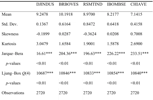
Table 1 reports the descriptive statistics. Comparing them, it shows that the standard deviation of each emerging index is higher than that of the DJINDUS, it implies the developed DJINDUS is relatively stable than those indices of the developing BRIC. In terms of the risk based on the deviation of the stock indices, it implies the risk of emerging stock markets of BRIC is relatively higher than that of the mature market of DJINDUS.

In addition, each index is non-normally distributed according to the Jarque–Bera normality test, and the Ljung–Box Q-statistics reveal that each series is significantly autocorrelated.

Figure 1. Logarithm of stock indices. DJINDUS BRBOVES RSMTIND IBOMBSE CHIAVE 6 7 8 9 10 11 12 2000 /1/3 2000/5 /3 2000/9 /3 2001/1 /3 2001 /5/3 2001/9 /3 2002 /1/3 2002/5 /3 2002 /9/3 2003/1 /3 2003/5 /3 2003/9 /3 2004/1 /3 2004/5 /3 2004/9 /3 2005/1 /3 2005/5 /3 2005 /9/3 2006/1 /3 2006 /5/3 2006/9 /3 2007 /1/3 2007/5 /3 2007/9 /3 2008/1 /3 2008/5 /3 2008/9 /3 2009/1 /3 2009 /5/3 2009/9 /3 2010 /1/3 2010/5 /3 _date lo g a ri th m o f st o ck in di ce s DJINDUS BRBOVES RSMTIND IBOMBSE CHIAVE

Table 1. Summary statistics for the stock indices.

DJINDUS BRBOVES RSMTIND IBOMBSE CHIAVE

Mean 9.2478 10.1918 8.9700 8.2177 7.1415 Std. Dev. 0.1367 0.6164 0.8472 0.6418 0.4158 Skewness -0.1899 0.0287 -0.3624 0.0208 0.7008 Kurtosis 3.0479 1.6584 1.9001 1.5878 2.6900 Jarque–Bera 16.61*** 204.36*** 196.63*** 226.22*** 233.51*** p-values <0.01 <0.01 <0.01 <0.01 <0.01 Ljung–Box Q(4) 10687*** 10846*** 10833*** 10854*** 10840*** p-values <0.01 <0.01 <0.01 <0.01 <0.01 Observations 2720 2720 2720 2720 2720

Notes: The symbols *, ** and *** denote significance at the 10%, 5% and 1% levels, respectively.

4.2 Unit Root Tests

As a preliminary analysis of cointegration, we conducted the unit root tests by using the conventional Augmented Dickey–Duller (ADF) test and the Phillips–Perron (PP) test to ensure they have the same order. The ADF and the PP tests use the null hypothesis of having a unit root versus the alternative of stationarity in the series. As seen in Table 2, all series in levels are insignificant to reject the null; whereas they are significant to reject the null when taken in the first differences. For instance, the ADF statistic of the DJINDUS is -2.15, it is not small enough to reject the null of unit root, it implies the series of DJINDUS in level is nonstationary; while taken in the first differences, the value of ADF statistic is -41.42 and small enough, significantly rejecting the null of unit root. It implies the DJINDUS is I(1) series. On another way, for robustness test, the study used the PP test to examine the DJINDUS series for stationarity. Under the alternative PP test, the conclusion of I(1) series for the DJINDUS is the same, as the Table 2 demonstrates.

The same procedure was conducted for the other four series of BRBOVES, RSMTIND, IBOMBSE and CHIAVE of the BRIC. Finally, it is shown that all series investigated in this study are integrated of order 1, satisfying the necessary condition for cointegration. More details can be found in the Table 2.

4.3

Engle–Granger cointegration test

Proceeding with the E–G methodology, the estimated attractor equations of (1) for US–BRIC are reported in Table 3. For the case of US–Brazil, the regression F-statistic is 907.6, the estimated constant 8.1172 and the coefficient 0.1109 are all significant at the 1% significance level. This indicates that the logarithm of BRBOVES moves by 1 and the logarithm of the DJINDUS moves by 11.09%. The other three cases had similar results.

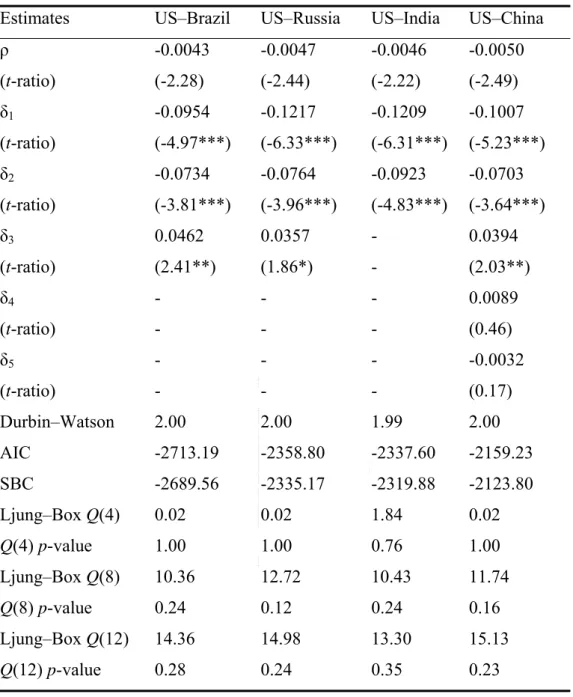
Next, the study estimated (2), with the results presented in Table 4. For the case of US–Brazil, in column 2 of Table 4, the results are appropriate for using three lagged terms based on the AIC or SBC. The Durbin–Watson statistic is 2.00 and the Ljung–Box statistics

Q(4), Q(8) and Q(12) reveal that there is no autocorrelation. The estimated coefficient ˆ is

-0.0043, while the corresponding E–G statistic is only -2.28, which is not small enough to reject the null of no cointegration when compared with the critical value -3.37 at the 5% significance level. This indicates that there is no long-run cointegration relationship for US–Brazil.

Similar situations occur in the other three cases, with no long-run cointegration relationships for the US–Russia, US–India, and US–China under the framework of the E–G cointegration test.

Table 2. Conventional unit root tests. Logarithm of stock index ADF PP Level Lag 1st

Difference Lag Level Bandwidth 1st Difference Bandwidth DJINDUS -2.15 2 -41.42*** 1 -2.44 1 -56.95*** 4 BRBOVES -2.41 0 -52.08*** 0 -2.33 19 -52.20*** 20 RSMTIND -1.40 0 -51.04*** 0 -1.35 17 -51.06*** 18 IBOMBSE -2.60 1 -48.30*** 0 -2.50 4 -48.29*** 3 CHIAVE -1.21 0 -51.61*** 0 -1.26 8 -51.65*** 8

Table 3. Four attractor equations.

Countries

Independent

Variable Coefficient t-statistic p-value F-statistic p-value US–Brazil Constant 8.1172 215.89*** <0.01 907.60*** <0.01 BRBOVES 0.1109 30.13*** <0.01 US–Russia Constant 8.6198 343.21*** <0.01 630.81*** <0.01 RSMTIND 0.0700 25.12*** <0.01 US–India Constant 8.3320 290.46*** <0.01 1025.46*** <0.01 IBOMBSE 0.1114 32.02*** <0.01 US–China Constant 8.2262 202.61*** <0.01 635.27*** <0.01 CHIAVE 0.1431 25.20*** <0.01

Notes: The dependent variable is DJINDUS. The four attractor equations are estimated from bilateral relationships of the US–Brazil, US–Russia, US–India, and US–China, respectively.

Table 4. Engle–Granger cointegration test.

Estimates US–Brazil US–Russia US–India US–China

ρ -0.0043 -0.0047 -0.0046 -0.0050 (t-ratio) (-2.28) (-2.44) (-2.22) (-2.49) δ1 -0.0954 -0.1217 -0.1209 -0.1007 (t-ratio) (-4.97***) (-6.33***) (-6.31***) (-5.23***) δ2 -0.0734 -0.0764 -0.0923 -0.0703 (t-ratio) (-3.81***) (-3.96***) (-4.83***) (-3.64***) δ3 0.0462 0.0357 - 0.0394 (t-ratio) (2.41**) (1.86*) - (2.03**) δ4 - - - 0.0089 (t-ratio) - - - (0.46) δ5 - - - -0.0032 (t-ratio) - - - (0.17) Durbin–Watson 2.00 2.00 1.99 2.00 AIC -2713.19 -2358.80 -2337.60 -2159.23 SBC -2689.56 -2335.17 -2319.88 -2123.80 Ljung–Box Q(4) 0.02 0.02 1.84 0.02 Q(4) p-value 1.00 1.00 0.76 1.00 Ljung–Box Q(8) 10.36 12.72 10.43 11.74 Q(8) p-value 0.24 0.12 0.24 0.16 Ljung–Box Q(12) 14.36 14.98 13.30 15.13 Q(12) p-value 0.28 0.24 0.35 0.23

Note: The critical value of Engle–Granger statistic at the 5% significance level is -3.37 (see Engle and Yoo, 1991).



4.4 Enders–Siklos asymmetric threshold cointegration test

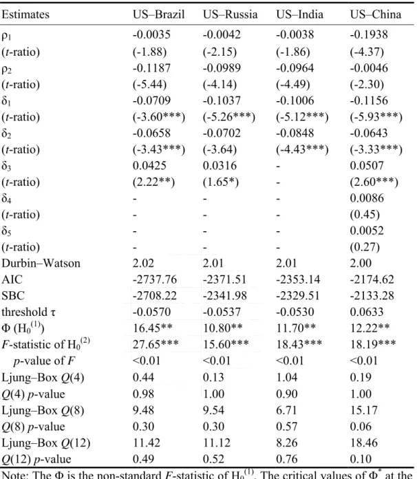
Although, the study found no cointegration under the E–G cointegration framework, to prevent errors of model misspecification, the study considered the possibility of nonlinearity in the cointegration relationship and evaluated the possibility of a threshold, using the powerful consistent M-TAR model (Enders and Siklos, 2001) to re-examine the cointegration relationships. The study reports the results in Table 5.

For the US–Brazil case, the estimated positive-deviation adjustment speed 1 is -0.0035,

and the negative-deviation adjustment speed 2 is -0.1187. Both speeds satisfy the necessary

condition of ₁ < 0, ₂ < 0 and the sufficient condition of (1₁)(1₂) 1 for convergence. The corresponding Durbin-Watson statistic is 2.02, and the Ljung–Box statistics

Q(4), Q(8), and Q(12) are all insignificant to reject the null of no autocorrelation. The AIC is

-2737.76 and the SBC is -2708.22; both are smaller than those of -2713.19 and -2689.56, respectively, under the E–G cointegration framework (as seen in the column 2 of the Table 4 for the US–Brazil). Using either the AIC or the SBC, the consistent M-TAR model is much more suitable for this situation since it obtains more information. For inference, the estimated  value, 16.45, and the F-value value, 27.65, are both large enough to reject the null of (1)

0

H and (2)

0

H , respectively. Lastly, the estimated consistent threshold  is -0.057.

For the case of US–Brazil, this implies that long-run asymmetric threshold cointegration relationship existed in the 2000s. The results also indicate that: 1) the asymmetry behaves differently in two regimes based on the threshold value -0.057; and 2) discrepancies from long-term equilibrium such that t1 0.057 are relatively eliminated slowly, whereas

found nonlinear cointegrating relationships in the long-run, as shown in the Table 5. Overall, in comparative analysis, the nonlinear cointegration with asymmetry better describes these relationships studied.

Table 5. Enders–Siklos consistent M-TAR cointegration test.

Estimates US–Brazil US–Russia US–India US–China

ρ1 -0.0035 -0.0042 -0.0038 -0.1938 (t-ratio) (-1.88) (-2.15) (-1.86) (-4.37) ρ2 -0.1187 -0.0989 -0.0964 -0.0046 (t-ratio) (-5.44) (-4.14) (-4.49) (-2.30) δ1 -0.0709 -0.1037 -0.1006 -0.1156 (t-ratio) (-3.60***) (-5.26***) (-5.12***) (-5.93***) δ2 -0.0658 -0.0702 -0.0848 -0.0643 (t-ratio) (-3.43***) (-3.64) (-4.43***) (-3.33***) δ3 0.0425 0.0316 - 0.0507 (t-ratio) (2.22**) (1.65*) - (2.60***) δ4 - - - 0.0086 (t-ratio) - - - (0.45) δ5 - - - 0.0052 (t-ratio) - - - (0.27) Durbin–Watson 2.02 2.01 2.01 2.00 AIC -2737.76 -2371.51 -2353.14 -2174.62 SBC -2708.22 -2341.98 -2329.51 -2133.28 threshold τ -0.0570 -0.0537 -0.0530 0.0633 Φ (H0(1)) 16.45** 10.80** 11.70** 12.22** F-statistic of H0(2) 27.65*** 15.60*** 18.43*** 18.19*** p-value of F <0.01 <0.01 <0.01 <0.01 Ljung–Box Q(4) 0.44 0.13 1.04 0.19 Q(4) p-value 0.98 1.00 0.90 1.00 Ljung–Box Q(8) 9.48 9.54 6.71 15.17 Q(8) p-value 0.30 0.30 0.57 0.06 Ljung–Box Q(12) 11.42 11.12 8.26 18.46 Q(12) p-value 0.49 0.52 0.76 0.10

Note: The Φ is the non-standard F-statistic of H0(1). The critical values of Φ* at the

5% significance level with no, one, and four lagged changes are 6.62, 6.63, 6.32, respectively (see Ender and Siklos, 2001).



4.5 Estimation of the threshold error correction model

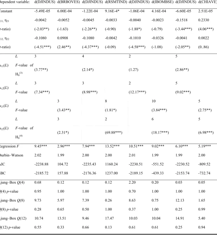
Based on the asymmetric cointegration relationships discovered, the study estimated the TECM, (5) and (6), with results as presented in Table 6.

As seen in the US–Brazil, equations of the d(DJINDUS) (corresponding to (5)) and the d(BRBOVES) (corresponding to (6)) were estimated, showing that the two nulls of (3)

0

H and

(4) 0

H are rejected at the 5% and 10% significance levels, respectively. The results show the return rate of BRBOVES significantly Granger-causes that of the DJINDUS in the short-run, while the return rate of DJINDUS weakly Granger-causes that of the BRBOVES at the 10% significance level.

The other cases are similar. For the US–Russia, the return rate of the RSMTIND weakly Granger-causes that of the DJINDUS at the 10% significance level, while the return rate of DJINDUS significantly Granger-causes that of the RSMTIND. In the US–India, there is only one Granger-causality direction: the return rate of the DJINDUS significantly Granger-causes that of the IBOMBSE. Overall, significant bi-directional Granger-causality relationships exist in the US–China, whereas they appear weakly in the US–Brazil and US–Russia.

Table 6. Estimated threshold error correction model.

US–Brazil US–Russia US–India US–China

Dependent variable: d(DJINDUS) d(BRBOVES) d(DJINDUS) d(RSMTIND) d(DJINDUS) d(IBOMBSE) d(DJINDUS) d(CHIAVE) Constant -5.49E-05 6.00E-04 -1.22E-04 9.16E-4* -1.06E-04 4.16E-04 -6.60E-05 2.51E-05 η11, η21 -0.0042 -0.0052 -0.0045 -0.0033 -0.0040 -0.0023 -0.1518 0.2330 (t-ratio) (-2.03**) (-1.63) (-2.26**) (-0.90) (-1.88*) (-0.79) (-3.44***) (4.06***) η12, η22 -0.1080 0.0908 -0.1080 -0.0042 -0.1010 -0.0326 -0.0041 0.0022 (t-ratio) (-4.51***) (2.46**) (-4.37***) (-0.09) (-4.58***) (-1.08) (-2.05**) (0..86) A11(L) L 3 4 2 5 F-value of H0(3) (3.77**) (2.14*) (1.27) (2.86**) A12(L) L 3 3 2 5 F-value (7.34***) (8.98***) (12.17***) (9.02***) A21(L) L 3 8 10 5 F-value (3.43**) (1.81*) (3.84***) (2.75**) A22(L) L 3 2 6 5 F-value of H0(4) (2.31*) (69.88***) (18.17***) (6.98***) Regression F 9.45*** 2.96*** 7.94*** 13.52*** 10.51*** 9.02*** 6.10*** 5.19*** Durbin–Watson 2.02 1.99 2.00 2.00 2.01 1.99 1.99 2.00 AIC -2238.88 104.72 -2235.43 1160.24 -2230.51 -551.52 -2230.52 -809.52 SBC -2185.72 157.88 -2176.36 1237.00 -2189.15 -439.33 -2153.74 -732.74 Ljung–Box Q(4) 0.68 0.12 0.12 0.12 2.20 0.20 0.03 0.05 Q(4) p-value 0.95 1.00 1.00 1.00 0.70 1.00 1.00 1.00 Ljung–Box Q(8) 9.73 5.97 7.39 0.26 8.63 0.75 12.13 1.65 Q(8) p-value 0.28 0.65 0.50 1.00 0.37 1.00 0.25 0.99 Ljung–Box Q(12) 10.74 13.51 9.46 17.47 10.03 10.04 14.91 5.40 Q(12) p-value 0.55 0.33 0.66 0.13 0.61 0.61 0.25 0.94

4.6 Time-varying asymmetric threshold cointegration by recursive

estimation

Figure 2 shows the plots of tested statistics Phi , SymF, F11 and F22 (corresponding to

the (1) 0 H , (2) 0 H , (3) 0 H and (4) 0

H ) in a recursive manner. Suitable lag lengths are selected via the AIC and BIC over the full sample period, as presented in Tables 5 and 6, for all sub-period estimations. The same practice of selecting the suited lag length can also be found in Lucey and Aggarwal (2010) who used the recursive method to study dynamic integration in European markets.

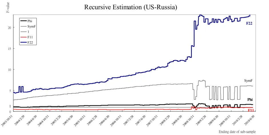
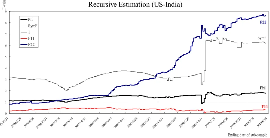
Consequently, as seen in the Figures 2–5, the Phi and the SymF sequences appear to

have similar types with different levels in all the four cases and they present obvious upward trends in the US–Brazil, US–India, and US–China. An upward trend indicates that the long-run nonlinear threshold cointegrating relationships are becoming stronger. Nevertheless, the Phi and the SymF dropped dramatically in 2008 and the cointegration relationships

broke down because there were possible structural breaks which changed the original situations. When the impacts of the crisis had reduced down, the relationships recovered quickly and returned to their original directions after 2008. Moreover, the long-run threshold cointegrating relationships along with the asymmetric adjustment pattern become more significant than previously for the US–Brazil (Figure 2), US–India (Figure 4), and US–China (Figure 5); but were variable for the US–Russia (Figure 3).

For the short-run relationships of the Granger-causality, the F11 values were not significant in the early 2000s for the BRIC, which implies the emerging stock markets do not dominate the US stock market at that time. Nevertheless, due to the rapid economic growth in the 2000s, the stock markets of Brazil, Russia and China began to influence the US to some

extent after 2006, as the F11 implies in the Figures 2, 3 and 5. As such, it was seen that the return rates of the BROBVES, RSMTIND and CHINAVE Granger-cause that of the Dow Jones index to a certain degree. Nonetheless, the IBOMBSE of India did not Granger-cause the Dow Jones over the past ten years, as the F11 implies in the Figure 4. On the other hand, when inspecting the F22, upward trends appear and become significant for the US–Russia, US–India, and US–China (Figures 3–5), except for the US–Brazil, where the F22 has declined recently (Figures 2). Overall, this implies the return rate of Dow Jones index increasingly Granger-causes those of the Russia, India, and China, and can be served as a leading indicator for short-run forecasting, though not for the US–Brazil.

Finally, recursive estimation demonstrates the dynamics of evolving pattern of the long-run cointegration and short-run Granger-causality relationships for the US–BRIC, accounting for the final outcomes reported in Tables 5 and 6.

Figure 2. Recursive Estimation of US–Brazil. Note: The critical value of Ö*

250, 5% is 6.63, the critical F-statistics used are: SymF3, 1000; 5%=2.61, F113, 1000; 5%=2.61,

F223, 1000; 5%=2.61.

Recursive Estimation (US-Brazil)

Phi SymF 1 F11 F22 0 2 4 6 8 10 12 2003 /10/31 2004 /2/29 2004 /6/30 2004 /10/31 2005 /2/28 2005 /6/30 2005 /10/31 2006 /2/28 2006 /6/30 2006 /10/31 2007 /2/28 2007 /6/30 2007 /10/31 2008 /2/29 2008 /6/30 2008 /10/31 2009 /2/28 2009 /6/30 2009 /10/31 2010 /2/28 2010 /6/30 Ending date of sub-sample

F-v al u e Phi SymF 1 F11 F22

Figure 3. Recursive Estimation of US–Russia.

Note: The critical F-statistics used are: SymF3,1000;5%=2.61, F114,1000;5%=2.37, F222,1000;5%=2.99.

Recursive Estimation (US-Russia)

Phi SymF 1 F11 F22 0 5 10 15 20 2003/ 10/31 2004 /2/29 2004/ 6/30 2004/ 10/31 2005 /2/2 8 2005 /6/3 0 2005 /10/31 2006 /2/28 2006 /6/30 2006/ 10/31 2007 /2/2 8 2007 /6/3 0 2007/ 10/31 2008 /2/2 9 2008 /6/30 2008/ 10/31 2009 /2/28 2009 /6/3 0 2009 /10/31 2010 /2/2 8 2010 /6/30

Ending date of sub-sample

F-va lu e Phi SymF 1 F11 F22

Figure 4. Recursive Estimation of US–India.

Note: The critical F-statistics used are: SymF2, 1000; 5%=2.99, F112, 1000; 5%=2.99, F226, 1000; 5%=2.1.

Recursive Estimation (US-India)

Phi SymF F11 F22 0 1 2 3 4 5 6 7 8 9 2003/10 /31 2004/ 2/29 2004/6/ 30 2004/1 0/31 2005/2/ 28 2005/ 6/30 2005/10 /31 2006/ 2/28 2006/ 6/30 2006/10 /31 2007/ 2/28 2007/6/ 30 2007/1 0/31 2008/2/ 29 2008/6 /30 2008/10 /31 2009/2/ 28 2009/6 /30 2009/10 /31 2010/2 /28 2010/6/ 30

Ending date of sub-sample

F-va lu e Phi SymF 1 F11 F22

Figure 5. Recursive Estimation of US–China.

Note: The critical F-statistics used are: SymF5, 1000; 5%=2.22, F115, 1000; 5%=2.22, F225, 1000; 5%=2.22. Recursive Estimation (US-China)

Phi SymF F11 F22 0 1 2 3 4 5 6 7 8 9 2003 /10/ 31 2004 /2/29 2004 /6/3 0 2004 /10/ 31 2005 /2/2 8 2005 /6/3 0 2005 /10/ 31 2006 /2/2 8 2006 /6/3 0 2006 /10/ 31 2007 /2/2 8 2007 /6/3 0 2007 /10/ 31 2008 /2/2 9 2008 /6/3 0 2008 /10/ 31 2009 /2/2 8 2009 /6/3 0 2009 /10/ 31 2010 /2/2 8 2010 /6/3 0

Ending date of sub-sample

F-value Phi SymF 1 F11 F22

4.7

Time-varying asymmetric threshold cointegration by rolling

estimation

The results for rolling estimation are plotted in Figures 6–9. As expected, the results are much more complex and sensitive than those from the recursive estimation plotted in Figure 2–5.

First, the study examined the rolling cointegration tests (as the Phi shows in Figure 6–9) and found that the nature of cointegrating relationship is much more time-varying when in the rolling manner. There is significant evidence over some sub-periods, but suddenly not over others. Nevertheless, the study still found that recently the nonlinear cointegrating relationships are becoming stronger in the US–Brazil, US–Russia and US–China (Figures 6, 7, and 9), but declining for the US–India (Figure 8).

As the SymF shows, the asymmetric adjustment test of H(2)0 indicates that there is

general statistical significance for all four cases, though it varies dramatically with no fixed pattern. Nevertheless, the asymmetry presents an increasing trend in the US–Brazil, US–Russia and US–China.

Another consideration is the short-run Granger-causality relationships, for which the study examined the test of _H(3)

o . As the F11 shows, the markets of Brazil and Russia significantly

Granger-cause the US after 2006 (Figures 6 and 7). The results of testing the _H(3)

o here are

not wholly consistent with those by the recursive estimation, since the rolling estimation here is much more sensitive. On the other hand, the F22, results show that the US increasingly Granger-causes the Russia, India, and China since the corresponding F22 sequences demonstrate upward trends with significance, but not for the Brazil.

Figure 6. Rolling Estimation of US–Brazil.

Rolling Estimation (US-Brazil)

Phi SymF F11 F22 0 1 2 3 4 5 6 7 8 9 10 2003 /10/31 2004 /2/29 2004 /6/30 2004 /10/31 2005 /2/28 2005 /6/30 2005 /10/31 2006 /2/28 2006 /6/30 2006 /10/31 2007 /2/28 2007 /6/30 2007 /10/31 2008 /2/29 2008 /6/30 2008 /10/31 2009 /2/28 2009 /6/30 2009 /10/31 2010 /2/28 2010 /6/30 Ending date of sub-sample

F-v al u e Phi SymF 1 F11 F22

Figure 7. Rolling Estimation of US–Russia.

Rolling Estimation (US-Russia)

Phi SymF 1 F11 F22 0 2 4 6 8 10 12 14 16 18 20 2003/ 10/31 2004/2/ 29 2004/6/ 30 2004/10 /31 2005 /2/28 2005 /6/30 2005 /10/31 2006/2/ 28 2006/6/ 30 2006 /10/31 2007/2/ 28 2007/6/ 30 2007 /10/31 2008/2/ 29 2008/6/ 30 2008/10 /31 2009 /2/28 2009/ 6/30 2009 /10/31 2010/2/ 28 2010/6/ 30

Ending date of sub-sample

F-v al u e Phi SymF 1 F11 F22

Figure 8. Rolling Estimation of US–India.

Rolling Estimation (US-India)

Phi SymF 1 F11 F22 -2 0 2 4 6 8 10 12 2003 /10/31 2004 /2/29 2004 /6/30 2004 /10/31 2005 /2/28 2005 /6/30 2005 /10/31 2006 /2/28 2006 /6/30 2006 /10/31 2007 /2/28 2007 /6/30 2007 /10/31 2008 /2/29 2008 /6/30 2008 /10/31 2009 /2/28 2009 /6/30 2009 /10/31 2010 /2/28 2010 /6/30

Ending date of sub-sample

F-v al u e Phi SymF 1 F11 F22

Figure 9. Rolling Estimation of US–China.

Rolling Estimation (US-China)

Phi SymF 1 F11 F22 0 2 4 6 8 10 12 2003 /10/31 2004 /2/29 2004 /6/30 2004 /10/31 2005 /2/28 2005 /6/30 2005 /10/31 2006 /2/28 2006 /6/30 2006 /10/31 2007 /2/28 2007 /6/30 2007 /10/31 2008 /2/29 2008 /6/30 2008 /10/31 2009 /2/28 2009 /6/30 2009 /10/31 2010 /2/28 2010 /6/30 Ending date of sub-sample

F-v al u e Phi SymF 1 F11 F22

4.8 Comparisons and interpretations of the dynamics among the

US–BRIC

The BRIC nations have owned plentiful natural resources, large populations and economic markets, with relatively cheap human resources; they also enjoy high economic growth and are regarded as promising economies. But, in spite of their similarities, our findings show that long-run and short-run interdependences with the US stock market exhibit differences among the BRIC.

First, according to the four long-run attractors (see Table 3) that have been identified for stationarity in the study, the regression coefficient of the US–China, 14.31%, is twice that of the US–Russia, which is 7.00%, the highest of all studied. It indicates the Chinese stock market, in average, is much more responsive to the Dow Jones than the other three markets; whereas the Russian stock market is the least responsive. This may be due to the extensive international trade relations between the US and China. Close international trade leads to market integration (Kearney and Lucey, 2004), which would indicate that cointegration relationships exist in their stock markets.

Secondly, the study found the degree of long-run asymmetric cointegration relationship for the US–Brazil is the highest among the BRIC (see the Φ in the Table 5) and it continued to strengthen, especially after the financial crisis of the subprime mortgage in the US(see the Figure 2). This may be due to open economic policies and relatively short geographic distance between the both countries, which results in closer interdependence in economic activities. Thus, the long-run cointegration relationships by the Φ test remain a relatively higher level than the other US–BRIC pairs.

least influential among the BRIC, since the IBOMBSE index did not Granger-cause the Dow Jones index at all in 2000s. Estimating both with full-sample and dynamic manners, the corresponding results consistently demonstrate the insignificant outcome, as the F-value of H0(3) shown in the Table 6 and the F11 implies in the Figures 4 and 8. On the contrary, the

Brazilian and Chinese stock indices are much more influential than those of Russia and India (see the F-value of H0(3) in the Table 6).

Lastly, for the short-run causality relationship from the US to the BRIC, the Russian and Indian stock markets are the most Granger-caused markets by the Dow Jones. Furthermore, we found the relationships have tightened in the past ten years for the US–Russia and US–India (see the F22 in the Figures 3 and 4). This indicates that the changes from the Dow Jones index easily affect the Russian and Indian stock markets in the short-run, which implies that the Dow Jones index may act as a leading indicator for investing funds in both stock markets. In addition, a similar result can be found in the US–China recently, which implies the interdependence between the US and the China stock markets has become tighter (see the

F22 in the Figure 5).

Finally, considering the influence of financial crisis of the subprime mortgage on the stock market cointegration, the evidence demonstrates that the nonlinear cointegrating relationships were disrupted and became insignificant in some sub-periods during 2007 - 2008 for the US–BRIC. This scenario can be found by dynamic estimations, especially for the US–Brazil, US–Russia and US–India (see Figures 2, 3 and 4). It implies that in the context of a financial crisis, the nonlinear cointegration relationship might face structural changes.

V. Conclusion

This article has investigated the dynamic relationships of the US–Brazil, US–Russia, US–India, and US–China stock markets in 2000s. The study applied the E–G (1987) cointegration test and the E–S (2001) asymmetric threshold cointegration test for comparative analysis. The study also applied two alternative time-varying procedures for dynamic analysis in order to explore the evolving patterns of both long-run cointegration and short-run Granger-causality relationships between the developed US and each of the developing BRIC stock markets.

The results suggest that the consistent M-TAR model is much more suitable to this situation to describe the cointegration relationships when asymmetry exists in the adjustment speed. Using dynamic analysis, the time-varying natures of cointegration and Granger-causality are captured and the study gain insight to the changing process of the stock market interdependence, instead of addressing only the final outcomes for partial conclusions.

Based on the findings, the evidence shows that there are nonlinear threshold cointegration relationships between the stock markets of the US and each of the BRIC nations. The results suggest that the time-varying nonlinear cointegration relationships exist between the stock markets studied, consenting to the argument for time-varying nature of cointegration proposed by Awokuse et al. (2009) and Lucey and Aggarwal (2010). The study found increasing degrees of long-run nonlinear cointegration relationship with asymmetry in the US–Brazil, US–India, US–Russia and US–China in 2000s, though the upward trend is relatively less for the US–Russia. For the short-run relationships, the evidence shows that the Brazil, Russia and China stock markets have begun Granger-causing the Dow Jones after 2006, exerting their short-run influences to a certain degree. On the other hand, the Dow Jones continues to play a leading role and increasingly Granger-causing the stock markets of Russia, India and China.

The study also found that the shock of the subprime mortgage crisis in the US during 2007 - 2008 generated a cross-market rebalancing effect on these markets, thereby co-moving the stock markets until a new balance had been achieved. The results reveal that the nonlinear cointegrating relationships were altered by the crisis.

Finally, we have presented an original empirical model which extends the E–S (2001) asymmetric threshold cointegration test by recursive and rolling estimation, and it was seen that the time-varying nature of long-run as well as short-run relationships. These findings have important implication since the potential benefits from international risk diversification might be limited or gradually diminished when investing in both the US and the BRIC. These benefits should now be re-considered due to the increasing degrees of interdependence between these markets.

References

Aktan, B., Mandaci, P. E., Kopurlu, B. S. and Ersener, B., 2009. Behaviour of emerging stock markets in the global financial meltdown: evidence from bric-a. African Journal of Business

Management, 3(7), 396–404.

Asgharian, H. and Nossman, M., 2011. Risk contagion among international stock markets.

Journal of International Money and Finance, 30, 22–38.

Anderson, H. M., 1997. Transaction costs and nonlinear adjustment towards equilibrium in the US treasury bill market. Oxford Bulletin of Economics and Statistics, 59, 465–484.

Awokuse, T. O., Chopra, A. and Bessler, D. A., 2009. Structural change and international stock market interdependence: evidence from Asia emerging markets. Economic Modelling, 26, 549–559.

Barari, M., 2004. Equity market integration in Latin America: a time-varying integration score analysis. International Review of Financial Analysis, 13, 649–668.

Chang, T., 2001. Are there any long-run benefits from international equity diversification for Taiwan investors diversifying in the equity markets of its major trading partners, Hong Kong, Japan, South Korea, Thailand and the USA? Applied Economics Letters, 8, 441–446.

Enders, W. and Falk, B., 1999. Confidence intervals for threshold autoregressive models, working paper, Iowa State University, Dept. of Economics.

Enders, W. and Granger, C. W. J., 1998. Unit-root tests and asymmetric adjustment with an example using the term structure of interest rates. Journal of Business & Economic Statistics, 16(3), 304–311.

Enders, W. and Siklos, P. L., 2001. Cointegration and threshold adjustment. Journal of

Business & Economic Statistics, 19(2), 166–176.

estimation, and testing. Econometrica 55, 251–276.

Engle, R. F. and Yoo, B. S., 1991. Forecasting and testing in co-integration systems, in

Long-run Economic Relationships (Eds) R. F. Engle and C. W. J. Granger, Oxford University

Press, Oxford, pp. 113–29.

Fernández-Serrano, J. L. and Sosvilla-Rivero, S., 2003. Modelling the linkages between US and Latin American stock markets. Applied Economics, 35(12), 1423–1434.

Hansen, B., 1997. Inference in TAR models, Studies in Nonlinear Dynamics and

Econometrics, 1, 119–131.

Ilyina, A., 2007. Portfolio Constraints and Contagion in Emerging Markets. IMF Staff Papers, 53 (3), 351–374.

Kearney, C. and Lucey, B. M., 2004. International equity market integration: theory, evidence and implications. International Review of Financial Analysis, 13, 571–583.

Liu, X., Song, H. and Romilly, P., 1997. Are Chinese stock markets efficient? A cointegration and causality analysis. Applied Economics Letters, 4(8), 511–515.

Lucey, B. and Aggarwal, R., 2010. Dynamics of equity market integration in Europe: impact of political economy events. Journal of Common Market Studies, 48(3), 641–660.

Menezes, R., Ferreira, N. B. and Mendes, D., 2006. Co-movements and asymmetric volatility in the Portuguese and U.S. stock markets. Nonlinear Dynamics, 44, 359–366.

Östermark, R. 2001. Multivariate cointegration analysis of the Finnish–Japanese stock markets. European Journal of Operational Research, 134, 498–507.

Rangvid, J., 2001. Increasing convergence among European stock markets? A recursive common stochastic trends analysis. Economics Letters, 71, 383–389.

Seabra, F. 2001. A cointegration analysis between Mercosur and international stock markets.

Applied Economics Letters, 8, 475–478.

MTAR analysis. Journal of Business, 79(6), 3153–3174.

Shen, C. H., Chen, C. F. and Chen, L. H., 2007. An empirical study of the asymmetric cointegration relationships among the Chinese stock markets. Applied Economics, 39(11), 1433–1445.