數位電視廣播之符號邊界偵測和佈散領航碼同步設計

國

立

交

通

大

學

電子工程學系

碩士論文

數位電視廣播之符號邊界偵測和佈散領

航碼同步設計

Design of Symbol Boundary Detection and

Scattered Pilot Synchronization for DVB-T/H

指導教授：周世傑 博士

研究生：劉瑋昌

數位電視廣播之符號邊界偵測和佈散領航碼同步設計

Design of Symbol Boundary Detection and Scattered Pilot

Synchronization for DVB-T/H

研究生：劉瑋昌 Student：Wei-Chang Liu

指導教授：周世傑 博士 Advisor：Dr. Shyh-Jye Jou

國立交通大學

電子工程學系

碩士論文

A Thesis

Submitted to Institute of Electronics Engineering College of Electrical Engineering

National Chiao Tung University in partial Fulfillment of the Requirements

for the Degree of Master

In

Electronics Engineering July 2005

Hsinchu, Taiwan, Republic of China

數位電視廣播之符號邊界偵測和佈散領航碼同

步設計

研究生：劉瑋昌 指導教授：周世傑 博士

國立交通大學電子工程學系

摘要

在地面數位電視廣播和手持式數位電視廣播系統中，盲目的傳輸的符號模 式、保護區間長度和符號邊界偵測佔了很重要的角色。同時快速佈散領航碼同步 也必須被用來增進系統同步的時間。這篇論文提出了一個使用單一硬體、無除法 的地面/手持式數位電視廣播盲目傳輸符號模式、保護區間長度和符號邊界偵測 合併架構。藉著使用龍捲風式記憶體存取法，本架構節省了 33%的記憶體面積和 41.6%的偵測時間。同時也提出一個兩階的快速佈散領航碼同步方法以增加快速 佈散領航碼同步演算法的可靠性。藉著預先存入通道估測所需之佈散領航碼，整 體的快速佈散領航碼同步時間可以被縮減 97.06%到 100%。最後，一個三階的解 映射和無除法通道補償器合併架構也被展現在此論文。

Design of Symbol Boundary Detection and

Scattered Pilot Synchronization for DVB-T/H

Student：Wei-Chang Liu Advisor：Dr. Shyh-Jye Jou

Institute of Electronics Engineering

National Chiao Tung University

Abstract

In DVB-T/H broadcasting system, blind mode, Guard Interval (GI) length detection and coarse symbol synchronization plays important roles to estimate the symbol parameters before TPS is decoded. Also fast scattered pilot synchronization is necessary to reduce the timing of synchronization. In this thesis, a single hardware and division-free architecture modified from Normalized-Maximum-Correlation (NMC) architecture for DVB-T/H mode/GI length detection and coarse symbol synchronization is proposed. By adopting the twister memory access method and a sequential mode detection scheme, the architecture reduces 33% memory cost and at most 41.6% detection latency. A two-stage fast scattered pilot synchronization scheme is also proposed to increase the reliability of scattered pilot synchronization. A channel estimation pilots pre-filling skill is added to the two-stage fast scattered pilot synchronization scheme. Thus the scattered pilot synchronization timing is reduced by at best 100% to 97.06%. Furthermore, a three-stage demapping embedded with division-free frequency domain equalizer (FEQ) scheme is also presented.

誌謝

首先必須感謝周世傑老師，在我大一、二的時候啟蒙了我進入電子組這個領 域。在研究所的兩年生涯中，給與我許多珍貴的知識和鼓勵。這兩年來，老師不 僅在研究上使我受益良多，在為人處事上、態度上、研究的精神上有給予我許多 難得的寶貴意見。 再者感謝劉建男老師和李進福老師，培養了我這方面的才能。對我的諄諄教 誨令我永遠銘記在心，使我能夠在這裡繼續努力。 又君、儒遠、俊豪，你們不止是大學時代的戰友，同時也是實驗室令人尊敬 的學長姐，給予我許多有用的建議，也陪伴我一路成長至今。 實驗室的伙伴們，偷偷龍、丸子、momo、老大、儷蓉、小朱、誌華、一哥、 Nirvana、阿賢、奕瑋、志雄、spice、俊男、阿樸、俊誼、晉欽和小趙。與你們 在一起的時間充滿著歡樂和汗水。 Vinson、文良、黃 yaya、昭龍、飯團和大師兄。這些自大學時代就與我一 起互相勉勵的伙伴們，沒有你們的支持我的研究所生涯也不會過得如此精彩。 研究所生涯中最重要的伙伴，庭禎、琪耀和一心。感謝你們在 DVB 研究上和 我一起努力打拼，並且提供我很多有用的意見和想法。 最後要感謝我的父母和女友的支持，使我可以安心無虞的度過這光輝的兩年 歲月。

Content

Chapter 1 Introduction...1

1.1 Overview of Digital TV Broadcasting ...1

1.2 DTV System in Taiwan - DVB-T/H ...2

1.3 Motivation...3

1.4 Thesis Organization ...4

Chapter 2 OFDM and DVB-T/H Technology ...5

2.1 Concept of OFDM ...5

2.2 DVB-T/H Technology...7

2.2.1 MPEG-2 Source Coding and Multiplexing ...7

2.2.2 Channel Coding ... 7

2.2.3 Mapper & Frame...9

2.2.4 Reference Signals ... 10

2.2.5 DVB-H Particular ...12

Chapter 3 Symbol Synchronization Algorithms...14

3.1 Mode/GI Detection ...15

3.1.1 Introduction to Mode/GI Detection ...15

3.1.2 Proposed Mode/GI Scheme ...20

3.1.3 Performance Simulation ...23

3.2 Coarse Symbol Synchronization...24

3.2.1 Effect of Symbol Timing Offset ...25

3.2.2 Coarse Symbol Synchronization Algorithms...27

3.2.3 Performance Simulation and Comparisons ...29

3.2.4 Proposed Mode/GI and Symbol Boundary Detection Scheme...33

Chapter 4 Channel Estimation Algorithms...39

4.1 Scattered Pilot Synchronization...39

4.1.1 Fast Scattered Pilot Synchronization Algorithms ...40

4.1.2 Performance Simulation and Comparisons ...41

4.1.3 Proposed Two-Stage Scattered Pilot Synchronization Scheme ...44

4.1.4 Proposed Scattered Pilots Pre-Filling Scheme ... 47

4.2 Frequency Domain Channel Estimation ...49

3.4.1 Frequency Domain Channel Estimation Algorithms...50

3.4.2 Performance Simulation and Comparisons ...55

4.3 Channel Compensation and Demapping...57

4.4 Timing Synchronization Scheme ...61

Chapter 5 Architecture Design and Implementation ...63

5.2 Mode/GI & Symbol Boundary Detection...63

5.2.1 SRAM Based Delay-Line ... 64

5.2.2 Correlation Circuits ...66

5.2.3 Moving Sum Circuits...67

5.2.4 Finite Word-Length Simulation ...67

5.3 Scattered Pilot Synchronization...68

5.4 Frequency Domain Channel Estimation ...69

5.4 Channel Compensation and Hard Demapper...71

5.4.1 Hardware Design ...71

5.4.2 Finite Word-Length Simulation ...72

5.5 Design and Implementation Results ...74

Chapter 6 Conclusion and Future Work ...76

List of Tables

Table 1-1 Comparisons of different broadcasting standards...2

Table 2-1 Continual pilot carrier position...11

Table 2-2 TPS signaling information and format...12

Table 2-3 Specification of DVB-T/H...13

Table 3-1 MC, NMC and MMSE boundary average/peak offset @ Ricean/Rayleigh 31 Table 3-2 Components required for MC, NMC and MMSE ...32

Table 3-3 Timing for mode/GI and boundary detection ...37

Table 4-1 Statistic of power-based and correlation-based architectures...44

Table 4-2 Latency of different combination ...45

Table 4-3 Summary of different SPS schemes for 2-D channel estimation...49

Table 4-4 Required storage elements of channel estimation algorithms ...55

Table 5-1 Area of four correlation delay-line realization methods ...66

Table 5-2 Possible B×NF values of stage 2 ...72

Table 5-3 Possible B×NF values of stage 3 ...72

Table 5-4 Design results...74

List of Figures

Fig. 2.1 Sub-channels in FDM modulation...5

Fig. 2.2 Sub-channels in OFDM modulation...5

Fig. 2.3 Received OFDM symbols with multipath effect...6

Fig. 2.4 Functional block diagram of DVB-T transmission system ...7

Fig. 2.5 Scrambler/descrambler schematic diagram ...8

Fig. 2.6 Conceptual diagram of the outer interleaver and deinterleaver...9

Fig. 2.7 The mother convolution code of rate 1/2...9

Fig. 2.8 Distribution of scattered pilots ...11

Fig. 3.1 Block diagram of DVB-T baseband inner receiver ...14

Fig. 3.2 2K/4K/8K correlation under 8K mode ...16

Fig. 3.3 2K/4K/8K correlation results under (a) 2K (b) 8K transmission mode ...18

Fig. 3.4 2K/4K/8K normalized correlation results under (a) 2K (b) 8K mode...19

Fig. 3.5 Detected guard interval length is (a) smaller (b) larger than transmitted...20

Fig. 3.6 2K/4K/8K squared normalized correlation under (a) 2K (b) 8K mode...23

Fig. 3.7 Error rate under different threshold of proposed mode/GI detection ...24

Fig. 3.8 Effect of multipath fading...25

Fig. 3.9 Sub-carriers of (a) early case and (b) late case for timing offset...26

Fig. 3.10 MMSE mode/GI detection under (a) 2K (b) 8K mode...29

Fig. 3.11 MMSE boundary detection under (a) 2K (b) 8K mode...29

Fig. 3.12 (a) MC, (b) NMC and (c) MMSE boundary offset distribution @ Ricean ..30

Fig. 3.13 (a) MC, (b) NMC and (c) MMSE boundary offset distribution @ Rayleigh ...31

Fig. 3.14 Block diagram of (a) MC (b) NMC and (c) MMSE...32

Fig. 3.15 Block diagram of mode/GI detection ...33

Fig. 3.16 Architecture of mode/GI and boundary detection scheme ...34

Fig. 3.17 Finite state machine of mode/GI and boundary detection scheme...35

Fig. 3.18 Timing of parallel (a) 2K, (b) 4K, (c) 8K, sequential (d) refill, (e) replenish and (f) proposed mode detection schemes ...37

Fig. 3.19 (a) 2K MC2, (b) 2K NMC, (c) 8K MC2 and (d) 8K NMC simulation of the proposed blind mode/GI boundary detection scheme...38

Fig. 4.1 Error rate of two SPS algorithms versus SNR with (a) 0 (b) 0.03 (c) 0.33 CFO ...42

Fig. 4.2 Architecture of (a) power-based (b) correlation-based SPS ...43

Fig. 4.3 Two-stage scattered pilot synchronization scheme...44

Fig. 4.4 Error rate of SPS algorithms versus SNR with (a) 0 (b) 0.03 (c) 0.33 CFO ..46

Fig. 4.6 Stored scattered pilots of 1-D channel estimation ...51

Fig. 4.7 Frequency domain linear interpolation of 1-D channel estimation ...51

Fig. 4.8 Stored scattered pilots of 2-D channel estimation ...52

Fig. 4.9 Time domain linear interpolation of 2-D channel estimation...52

Fig. 4.10 Frequency domain linear interpolation of 2-D channel estimation ...53

Fig. 4.11 Stored scattered pilots of predictive 2-D channel estimation ...54

Fig. 4.12 Time domain linear interpolation of predictive 2-D channel estimation...54

Fig. 4.13 Freq. domain linear interpolation of predictive 2-D channel estimation...54

Fig. 4.14 BER under (a) static and (b) dynamic Channel...55

Fig. 4.15 Division simplification results in QAM ...59

Fig. 4.16 (a) FSM and (b) block diagram of hard demapping ...60

Fig. 4.17 Decision boundary of (a) stage 2 and (b) stage 3 ...61

Fig. 4.18 Example of three-stage demapping process ...61

Fig. 4.19 Demodulation flow ...62

Fig. 5.1 Architecture of DVB-T inner receiver...63

Fig. 5.2 R/W operation of dual and single port SRAM-based delay-line...64

Fig. 5.3 2K delay-line application...65

Fig. 5.4 Twister memory access operation...65

Fig. 5.5 Complex multiplier reduction...67

Fig. 5.6 MC2 results (a) before (b) after finite word-length simulation...68

Fig. 5.7 Improved architecture of blind mode/GI and boundary detection ...68

Fig. 5.8 Improved architecture of scattered pilot mode detection ...69

Fig. 5.9 Scattered pilot R/W conflict ...70

Fig. 5.10 Frequency domain interpolation...71

Fig. 5.11 Architecture of channel estimation ...71

Fig. 5.12 Finite word-length of BER after demapping ...73

Fig. 5.13 Architecture of stage-1...73

Fig. 5.14 Architecture of (a) stage-2 and (b) stage-3 ...73

Chapter 1

Introduction

1.1 Overview of Digital TV Broadcasting

Recently, thanks to the fast growing of VLSI technology, information technology and transmission technology, digital television (DTV) systems are going to replace traditional analogue television systems. By using digital compression, digital television systems can provide a HDTV (High Definition TV) program or four to six SDTV (Standard TV) programs in the same traditional channel bandwidth (6MHz). Digital television systems also have the ability to eliminate common analog broadcasting phenomenon such as “ghosting”, “snow” and static noises in audio. Therefore, digital television systems provide a high quality image and sound for consumers.

In the last few years, many standards for Digital TV Broadcasting are proposed with different performance of digital signal transmission. Such as DVB-T [1] (Digital Video Broadcasting-Terrestrial, Europe), ATSC [5] (Advanced Television System Committer, USA), ISDB-T [6] (Integrated Services Digital Broadcasting-Terrestrial, Japan). All above were recognized by ITU (International Telecommunication Union). For the portable devices, mobile phone and mobile TV for example, handheld standard such as DVB-H [2] (Digital Video Broadcasting-Handheld) is proposed by European Telecommunication Standard Institute (ESTI). Currently, another handheld standard T-DMB [7] (Terrestrial Digital Multimedia Broadcasting) has been to put into use in a number of countries. Table 1-1 lists the comparisons of above standards.

Table 1-1 Comparisons of different broadcasting standards

Standard DVB-T/H ATSC ISDB-T T-DMB

Modulation COFDM 8-VSB COFDM COFDM

Video MPEG-2 MPEG-2 MPEG-2 H.264

Audio ACC AC-3 ACC BSAC

Bandwidth 5/6/7/8MHz 6MHz 6MHz 1.5MHz

1.2 DTV System in Taiwan - DVB-T/H

ATSC has once adopted as Taiwan’s DTV standard in 1998. But by the effort of CTV, PTS, FTV, TTC and CTS, DVB-T was finally adopted to be the standard in year 2001. In year 2005 DVB-H was also adopted as mobile TV standard. As a result, DVB-T/H has become a hot topic in Taiwan. In May 2005, DTV system was broadcasted in west Taiwan. The E-Taiwan proposal plans start to retrieve analog channels in 2006. In 2010, TV broadcasting will become all in digital [8] [9].

Digital Video Broadcasting (DVB) was published by Joint Technical Committee (JTC) of European Telecommunication Standard Institute (ESTI), European Committee for Electrotechnical Standardization (CENELEC) and European Broadcasting Union (EBU). DVB family includes DVB-S (Satellite) [3], DVB-C (Cable) [4], DVB-T (Terrestrial) [1] and DVB-H (Handheld) [2]. DVB-T was published in 1997 with COFDM (Coded Orthogonal Frequency Division Multiplexing) transmission technique. Now there are many countries, such as UK, Germany, Norway, Australia, South Africa, India and Taiwan use DVB-T as their DTV transmission standard.

Though DVB-T can be applied in mobile environment, the power consumption is not good enough for portable devices. As a result, DVB-H was proposed for low power design and adopted for portable devices.

1.3 Motivation

Since the government of Taiwan adopted DVB-T as DTV standard and decides to revoke all analog channels in 2010, DVB-T products have become a very hot research topic now. Some products on market are based on DSP and others on ASIC [10]~[13]. For the purpose to be compatible with DVB-H, a low power version must be proposed. Since DVB-T/H receiver design is very important for portable devices, the ASIC design approach is preferred because it has lower power consumption than DSP based approach.

As many recently communication system such as ADSL (Asymmetric Digital Subscriber Line), DAB (Digital Audio Broadcasting) and WLAN (Wireless Local Area Network), DVB-T/H also uses OFDM technology. The benefits of OFDM includes high spectrum efficient by orthogonal technology, ability to against multipath interference (Fading) by inserting guard interval and cyclic prefix and can be transmitted in single frequency network (SFN). However time-variant channel will cause a loss in sub-carrier orthogonality and system performance due to the sub-carriers are spaced too close.

In broadcasting environment, DVB-T/H must solve the following problems. Transmission mode and Guard Interval (GI) mode detection is an important step at the beginning of system. Wrong transmission or GI mode decision will cause the whole system failed as a result of sending incorrect data to Fast Fourier Transform (FFT) module and get incorrect outputs. Accurate symbol boundary detection also plays an important role in DVB-T/H system. Without accurate symbol boundary, the sub-carriers may have a phase rotation or loss their orthogonality. Since DVB-T/H suffers from multipath interference and time-variant channel, the system need to extract the inserted scattered pilots and use the scattered pilots to compensate the

sub-carriers degradation by a frequency domain equalizer (FEQ). Scattered pilots synchronization (SPS) is a way to determine the current scattered pilot mode and reduce the timing to demapping. Other synchronization schemes such as carrier frequency offset (CFO) and sampling clock offset (SCO) are referred in [14].

This thesis proposes an efficient memory shared and division-free synchronization architecture which reduces the memory storage requirement. A Maximum-Correlation (MC) and Normalized-Maximum-Correlation (NMC) compromised architecture is proposed in this thesis to detect the transmission mode and guard interval length accurately and easily. Since Power-Based (PB) scattered pilot synchronization is weak in against noise, a two-stage scattered pilot synchronization scheme with channel estimation scattered pilots pre-filling method is also proposed in this thesis to improve the reliability and timing. Finally, a three-stage demapping architecture with embedded division-free FEQ is designed and it makes the whole architecture proposed in this these is a division-free architecture.

1.4 Thesis Organization

The following of this thesis is organized as follows. In chapter 2, OFDM will be introduced briefly and DVB-T/H technology will be discussed. Chapter 3 describes the effect of incorrect transmission/GI mode and detected boundary offset. Moreover, some algorithms, simulation and architectures for mode/GI detection and coarse symbol synchronization will be compared. A blind mode/GI and boundary detection scheme will be proposed. Algorithms, performance simulation and proposed scheme for scattered pilot synchronization, channel estimation and demapping will be discussed in Chapter 4. The architecture and hardware design will be presented in chapter 5. Finally, chapter 6 will give our conclusions and future works.

Chapter 2

OFDM and DVB-T/H Technology

2.1 Concept of OFDM

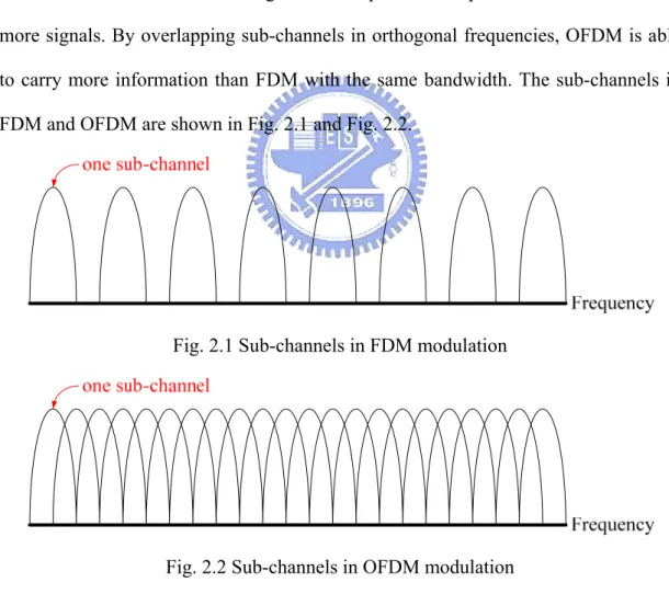
In mid 60s, frequency division multiplexing (FDM) was published. In FDM, multiple signals are sent at the same time with different sub-channels. OFDM [15] is based on this idea and uses orthogonal technique to overlap the sub-channels to send more signals. By overlapping sub-channels in orthogonal frequencies, OFDM is able to carry more information than FDM with the same bandwidth. The sub-channels in FDM and OFDM are shown in Fig. 2.1 and Fig. 2.2.

Fig. 2.1 Sub-channels in FDM modulation

Fig. 2.2 Sub-channels in OFDM modulation

OFDM with channel coding is called COFDM (Coded OFDM). The COFDM technique adopted by DVB-T, has the ability to reduce the ICI (Inter-Carrier Interference) and ISI (Inter-Symbol Interference) by inserting guard intervals (GI), a

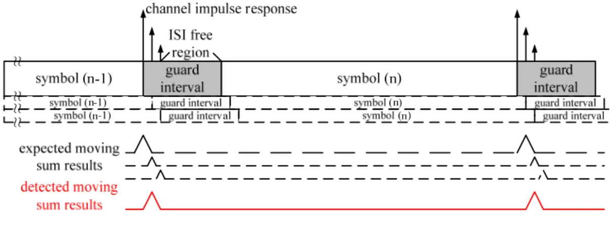
copy of the last period of the same OFDM symbol, between successive OFDM symbols. Since the multipath effect will cause the ISI phenomenon, to insert a guard interval is able to prevent the damage from other sub-paths. With inaccurate symbol detection, system has a high probability to find a wrong boundary which may allocate near the correct one. Owing to the difficulty of finding accurate boundary with multipath effect, system must tolerate to the inaccurate symbol boundary location. Therefore, the guard interval is filled by the copy of last period of a symbol. By using this characteristic, the detected boundary which locates before the correct one is able to decode correctly. Since the detected boundary locates before the correct one, according to OFDM mathematical function, the transmitted pattern looks like a cyclic shift without destroying the orthogonality of sub-carriers and will only cause a phase rotation. But if the detected boundary locates after the correct one, the sub-carriers will lose its orthogonality and lead to a wrong decoded answer. The received symbols with multipath effect are shown in Fig. 2.3.

symbol (n-1) symbol (n) symbol (n+1) transmitted symbol (n)

symbol (n-1) guard interval symbol (n)

＋

guard interval symbol (n+1)

main path multipath 1 multipath 2 multipath 3 received data guard interval

symbol (n-1) symbol (n) symbol (n+1) useable part useable part

destroyed part guard interval

＋

symbol (n-1) guard interval symbol (n) guard interval symbol (n+1)

＋

symbol (n-1) guard interval symbol (n)

＝

guard interval symbol (n+1)

2.2 DVB-T/H Technology

2.2.1 MPEG-2 Source Coding and Multiplexing

DVB-T is a broadcasting system based on OFDM modulation technology. Generally, this system can be divided into two parts, transmitter and receiver. In Fig. 2.4, a DVB-T transmission system block diagram is presented. MPEG-2 source coding and multiplexing multiplexes video, audio and data into an MPEG-2 program stream. Encoder Encoder MUX adaptation Energy dispersal Outer coder Outer interleaver Inner coder Inner interleaver Mapper Pilots & TPS signals Frame adapation OFDM Guard interval insertion D/A Front end ……… ……… MPEG-2 source coding and multiplexing

Transport MUXes

To aerial

TERRESTRIAL CHANNEL ADAPTER Encoder Encoder MUX adaptation Energy dispersal Outer coder Outer interleaver Inner coder

Fig. 2.4 Functional block diagram of DVB-T transmission system

2.2.2 Channel Coding

Channel coding includes randomizer, outer coder, outer interleaver, inner coder and inner interleaver. The MPEG-2 transport stream will be separated into high-priority (real line in Fig. 2.4) and low-priority (dotted line in Fig. 2.4). Therefore, in a small size monitor or weak signal environment, the receiver can switch a HDTV program into a SDTV program.

The MPEG-2 transport stream is organized as fixed length packets (118 bytes) and decorrelated by the block “MUX adaptation and energy dispersal”. Considering about the MPEG-2 Transport Stream have a probability to be a long 1 or 0 sequences, there will be some problem in synchronization. Doing Exclusive-OR operation with PRBS sequences can efficiently reach energy dispersal and randomize the MPEG-2 Transport Stream sequences. Fig. 2.5 illustrates the energy dispersal schematic diagram.

Fig. 2.5 Scrambler/descrambler schematic diagram

Outer coder uses a nonbinary block code, Reed-Solomon RS (240,188, t=8) shorten code, which have an ability to correct up to eight errors, with generator polynomial as Eqn. (2.1) is the usually used coding scheme recently.

1 )

(_{x = x}8_+x4_+x3_+x2₊

p (2.1)

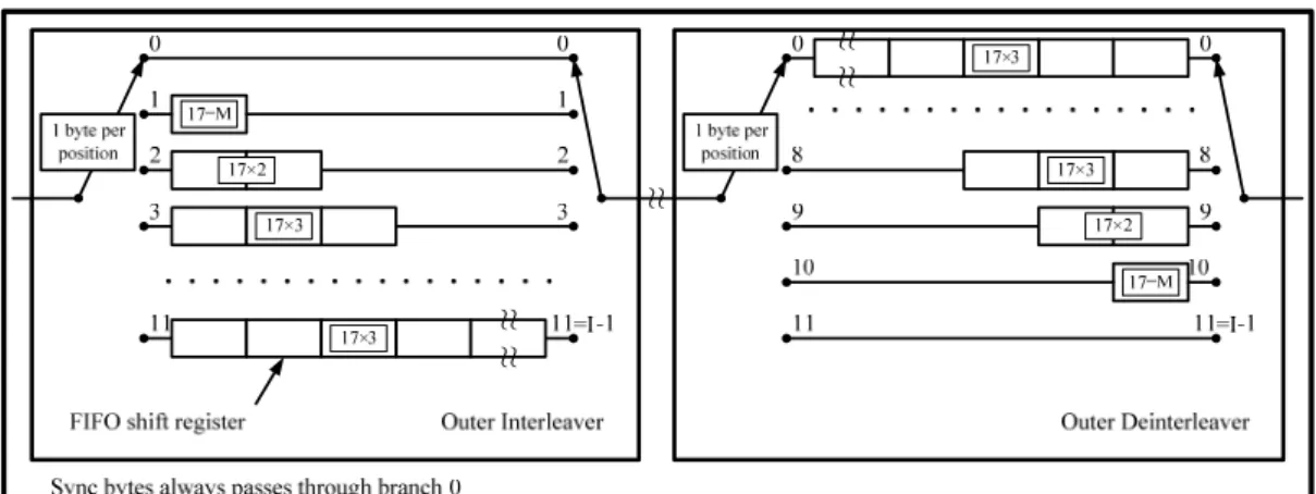
A convolutional byte-wise interleaving with depth I=12 is applied to make the transmitted data sequence being rugged to long sequences of errors. While transmission in air, a suddenly short period interference may occur because of many know or unknown reasons. Though RS have an ability to correct no more than 8 errors, the interference above is possibly lead to more than 8 errors in a RS package and unable to correct. At this time the outer interleaver opposites to this situation by interleaving the data in a symbol to other symbols. Fig. 2.6 is the conceptual diagram of the outer interleaver and deinterleaver.

≈

≈

≈

≈

≈

Fig. 2.6 Conceptual diagram of the outer interleaver and deinterleaver

For the purpose to have better Bit-Error-Rate (BER), a punctured convolutional encoder is cascaded with five valid coding rates: 1/2, 2/3, 3/4, 5/6, and 7/8. Higher coding rate means lower correction ability. Fig. 2.7 is an example of 1/2 coding rate which means one of two bits is useful.

Fig. 2.7 The mother convolution code of rate 1/2

Finally, a block based bit-wise inner interleaver is used to against the Viterbi output burst errors.

2.2.3 Mapper & Frame

After two level channel coding, all data carriers in an OFDM symbol will be mapped onto QPSK, 16-QAM, 64-QAM, non-uniform 16-QAM or non-uniform

64-QAM by the mapper. DVB-T provides 2 transmission modes, 2K mode and 8K mode. In DVB-H a 4K transmission mode is specially provided. Each frame consists of 68 OFDM symbols and contains scattered pilot cells, continual pilot carriers and TPS carriers. Four frames constitute one super-frame.

2.2.4 Reference Signals

Reference signals can be classed as three types, scattered pilot cells, continual pilot carriers and TPS carriers. All of them are inserted in all OFDM symbols. Scattered pilot cells do not really have a fixed position in a symbol but others do. The positions scattered pilot cells locates are as Eqn. (2.2) shows.

] ; [ , 0 , int | 12 } 4 mod ( 3

{k =K_min + × l + p p eger p≥ k∈ K_min K_max (2.2)

where k is the frequency index of the sub-carriers and l is the time index of the symbols. And it’s easy to seem that, scattered pilot cells’ location will be the same every four symbol. For different transmission mode, Kmax is different. Eqn. (2.3) shows how to generate scattered pilot cells’ value.

0 } Im{ ) 2 / 1 ( 2 3 / 4 } Re{ , , , , = − × = k l m k k l m c w c (2.3)

where wk is the kth data generated by PRBS.

In summary, Fig. 2.8 shows the distribution of scattered pilots. According to regular fixed located characteristic, scattered pilots can be used for channel estimation. By using timing interpolation, channel response can be reduced to 1/3.

Fig. 2.8 Distribution of scattered pilots

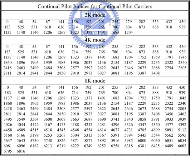
The locations of continual pilot carriers are listed in Table 2-1. The values of continual pilots are generated like that of Eqn. (2.3). The main function of continual pilots is to track carrier frequency offset.

Table 2-1 Continual pilot carrier position Continual Pilot Indices for Continual Pilot Carriers

2K mode 0 48 54 87 141 156 192 201 255 279 282 333 432 450 183 525 531 618 636 714 759 765 780 804 873 888 918 939 1137 1140 1146 1206 1269 1323 1377 1491 1683 1704 4K mode 0 48 54 87 141 156 192 201 255 279 282 333 432 450 183 525 531 618 636 714 759 765 780 804 873 888 918 939 1137 1140 1146 1206 1269 1323 1377 1491 1683 1704 1752 1759 1791 1845 1860 1896 1905 1959 1983 1986 2037 2136 2154 2187 2229 2235 2322 2340 2418 2463 2469 2484 2508 2577 2592 2622 2643 2646 2673 2688 2754 2805 2811 2814 2841 2844 2850 2910 2973 3027 3081 3195 3387 3408 8K mode 0 48 54 87 141 156 192 201 255 279 282 333 432 450 183 525 531 618 636 714 759 765 780 804 873 888 918 939 1137 1140 1146 1206 1269 1323 1377 1491 1683 1704 1752 1759 1791 1845 1860 1896 1905 1959 1983 1986 2037 2136 2154 2187 2229 2235 2322 2340 2418 2463 2469 2484 2508 2577 2592 2622 2643 2646 2673 2688 2754 2805 2811 2814 2841 2844 2850 2910 2973 3027 3081 3195 3387 3408 3456 3462 3495 3549 3564 3600 3609 3663 3687 3690 3741 3840 3858 3891 3933 3939 4026 4044 4122 4167 4173 4188 4212 4281 4296 4326 4347 4350 4377 4392 4458 4509 4515 4518 4545 4548 4554 4614 4677 4731 4785 4899 5091 5112 5160 5166 5199 5253 5268 5304 5313 5367 5391 5394 5445 5544 5562 5595 5637 5643 5730 5748 5826 5871 5877 5892 5916 5985 6000 6030 6051 6054 6081 6096 6162 6213 6219 6222 6249 6252 6258 6318 6381 6435 6489 6603 6795 6816

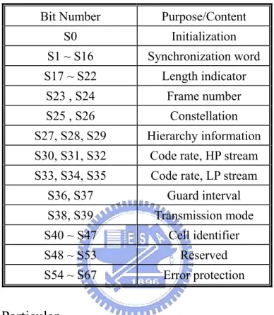
TPS pilots plays an important rule in DVB-T because of there is no any handshaking before communication. TPS pilots carry 68 different messages in a frame and the messages are listed in Table 2-2.

Table 2-2 TPS signaling information and format

Bit Number Purpose/Content

S0 Initialization S1 ~ S16 Synchronization word S17 ~ S22 Length indicator S23 , S24 Frame number S25 , S26 Constellation S27, S28, S29 Hierarchy information

S30, S31, S32 Code rate, HP stream

S33, S34, S35 Code rate, LP stream

S36, S37 Guard interval S38, S39 Transmission mode S40 ~ S47 Cell identifier S48 ~ S53 Reserved S54 ~ S67 Error protection

2.2.5 DVB-H Particular

For portable devices, time slicing technology is employed to reduce power consumption. For the purpose to improve the system performance in mobile environment, forward error correction for multiprotocol encapsulated data (MPE-FEC) is adopted with powerful channeling and time interleaving. Since 8K mode has better performance in large single frequency network (SFN) but worse in against Doppler Effect and 2K mode has better performance in against Doppler Effect but not suitable for large SFN, a comprised 4k mode is proposed. Overall, the specification of DVB-T/H is listed in Table 2-3.

Table 2-3 Specification of DVB-T/H

Transmission mode 2K, 4K, 8K

Number of useful sub-carriers 1705, 3409, 6817

Number of continual pilots 45, 89, 177

Number of scattered pilots 141, 282, 564

Number of TPS pilots 17, 34, 68

Radio frequency (MHz) 45~860

Guard interval 1/4, 1/8, 1/16, 1/32

Bandwidth (MHz) 5, 6, 7, 8

Elementary period (us) 7/40, 7/48, 7/56, 7/64

Channel model Rayleigh, Ricean

Forward error correct Convolution code with puncturing

Reed Solomon Code (204,188)

Constellation QPSK, 16QAM, 64QAM, non-uniform

16QAM, non-uniform 16QAM

Required BER 2 X 10-4 after Viterbi decoder

Chapter 3

Symbol Synchronization Algorithms

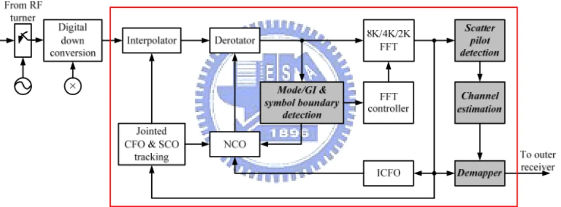
Fig. 3.1 illustrates the block diagram of DVB-T baseband inner receiver and all synchronization processes in digital domain. The block diagram contains mode/GI & symbol boundary detection, carrier synchronization loop, sampling synchronization loop, frequency domain channel estimation/compensation and hard demapper. This thesis will design the architecture based on this block diagram and focuses on the highlighted blocks.

Fig. 3.1 Block diagram of DVB-T baseband inner receiver

Timing synchronization plays an important role in digital communication systems. Without accurate timing synchronization process, the systems will fail to work in the beginning or get unreliable outcome. Timing synchronization includes mode/GI detection, coarse symbol synchronization (CSS), scattered pilot synchronization (SPS), carrier frequency offset (CFO) and sampling clock offset (SCO) issues. The last two topics have been discussed in [14]. This chapter focuses on mode/GI detection and coarse symbol synchronization problems. These two jobs should be down first in receiver. The FFT window has to decide the window length and locations with the correct transmission mode, guard interval length and symbol

boundary information. Otherwise, the feedback loops will have no idea to recover CFO and SCO and so do those parts behind inner receiver.

The goal of mode/GI detection is to get precise mode/GI parameters of transmitted symbols. By using the detected transmission mode, the system is able to set a FFT window, which length equals to transmission mode. Transmission mode and guard interval parameters make the system being able to compute boundaries behind the first boundary detected by coarse symbol synchronization. After mode/GI detection, coarse symbol synchronization process will adopt the parameters from mode/GI detection to do more accurate symbol boundary detection for the purpose to reduce timing offset effects and avoid ISI effect. Moreover, the results from mode/GI detection and coarse symbol synchronization make the system have enough information to determine the FFT window locations.

3.1 Mode/GI Detection

It seems that the system can get the information of transmission mode and guard interval length from TPS pilots discussed in 2.2.4. But without these messages, how can the systems set a correct FFT window length and correct FFT window locations? That means FFT has no idea to start to work and leads to no TPS information. This phenomenon will become a vicious cycle and system will never start to work. In order to make the FFT start to work, it’s necessary to do blind mode/GI detection before other processes of inner receiver.

3.1.1 Introduction to Mode/GI Detection

Mode/GI detection algorithms are usually similar to coarse symbol synchronization theorems. There are many methods to detect the mode/GI. For example, [16] proposed a blind transmission mode detection process, [17] modified a

mode/GI jointed detection process based on [16] and a two-stage mode/GI detection is discussed in [18].

a) Mode Detection

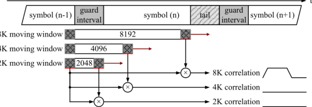
The basic idea of mode detection is to use the characteristic of the inserted guard intervals, a copy of tail in OFDM symbols. After surviving from fading channel, the guard interval part will still have a high correlation with symbol’s tail. Fortunately, other parts will have low or even no correlation with guard interval. Thus, for a 2K transmission mode, the mode detector shall find the correlation of r(n) and r(n-2K), where r(n) is the nth received signal. For the purpose to ensure the correlation result, to accumulate the correlation results between r(n)×r(n-2K) and r(n+64)×r(n-2K+64)

is necessary. Therefore, 2K+2×64, 4K+2×64 and 8K+2×64 long moving windows are required to detect the 2K/4K/8K transmission modes for DVB-T/H mode detection. Fig. 3.2 illustrates a simple diagram of the correlation results of 2K/4K/8K mode detection windows under 8K transmitted symbols. As the figure shows, only the 8K mode window is possibly located at the region of guard interval and symbol’s tail at the same time and will have prominent correlation results. Eqn. (3.1) presents the computation required in Fig. 3.2 mathematically.

guard

interval symbol (n) tail

2K correlation 4K correlation 8K correlation guard interval symbol (n-1) symbol (n+1) 8192 4096 2048 × 8K moving window 4K moving window 2K moving window × × t

Fig. 3.2 2K/4K/8K correlation under 8K mode

∑

= − − × − = 63 0 *_{( ) ( )} ) ( i N i n r i n r n x (3.1)

where N is the delay-line length which value will be 2K, 4K or 8K according to different transmission mode, r(n) is the received nth signal. Eqn. (3.2) is a modified version of Eqn. (3.1). By using an integration length equals to the minimum guard interval length of each tested transmission mode, the detector is able to have a reliable correlation result.

∑

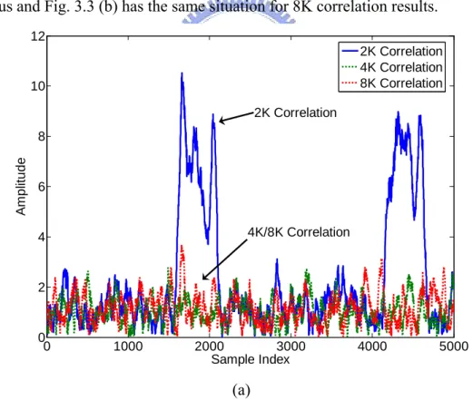
− = − − × − = 1 32 0 *_{( ) ( )} ) ( N i N i n r i n r n x (3.2)

Fig. 3.3 (a) and (b) show the different correlation results under different transmission modes with 1/4 guard interval, 12dB SNR, CFO=23.33 and surviving from Rayleigh channel. In Fig. 3.3 (a) only 2K correlation results have apparent plateaus and Fig. 3.3 (b) has the same situation for 8K correlation results.

0 1000 2000 3000 4000 5000 0 2 4 6 8 10 12 A m p lit u d e Sample Index 2K Correlation 4K Correlation 8K Correlation 2K Correlation 4K/8K Correlation (a)

0 0.5 1 1.5 2 x 104 0 2 4 6 8 10 12 A m pl itud e Sample Index 2K Correlation 4K Correlation 8K Correlation 8K Correlation 2K/4K Correlation (b)

Fig. 3.3 2K/4K/8K correlation results under (a) 2K (b) 8K transmission mode Even though Eqn. (3.1) or Eqn. (3.2) have the ability to distinguish the transmission mode, there is still some aliasing peaks occurred due to channel noise and may possibly lead to a wrong detected mode. For example, in Fig. 3.3 (a), there is an aliasing peak near sample index 3000 of 2K correlation results which is almost as high as the lowest plateau value near to sample index 2000 for 2K. Thus it is a problem to decide the peak or plateau threshold since there is no flat plateau and unitary plateau value.

To eliminate the effect from channel noises and ease the decision of the threshold, [17] used a normalized method to detect the transmission mode shown in Eqn. (3.3).

∑

∑

− = − = − × − − − × − = 1 32 0 * 1 32 0 * ) ( ) ( ) ( ) ( ) ( _N i N i i n r i n r N i n r i n r n x (3.3)

term. Fig. 3.4 (a) and (b) are the results of Eqn. (3.3), using the same pattern with Fig. 3.3. The plateau is ideally close to “1” and no other aliasing correlation results are higher than “0.707”. The characteristic of the normalized flat plateau can be also used to calculate the guard interval length and it will be discussed later.

0 1000 2000 3000 4000 5000 0 0.2 0.4 0.6 0.8 1 A m p lit u d e Sample Index 2K Correlation 4K Correlation 8K Correlation 2K Correlation 4K/8K Correlation (a) 0 0.5 1 1.5 2 x 104 0 0.2 0.4 0.6 0.8 1 A m pli tud e Sample Index 2K Correlation 4K Correlation 8K Correlation 8K Correlation 2K/4K Correlation (b)

b) Guard Interval Length Detection

The guard interval length will be detected after transmission mode. With an incorrect guard interval length, FFT won’t get correct patterns and sub-carriers after FFT won’t be the same with transmitted. Fig. 3.5 illustrates the situations of incorrect guard interval length. In Fig. 3.5 (a), a smaller guard interval length is detected and the second FFT window has a probability to get signals form the ISI destroyed region. The third FFT window gets some signals from the correct symbol, some from ISI destroyed region and others from previous symbol, this will lose the orthogonality of OFDM symbols and FFT outputs are absolutely incorrect. FFT windows in Fig. 3.5 (b) also get incorrect signals either.

(a)

(b)

Fig. 3.5 Detected guard interval length is (a) smaller (b) larger than transmitted [18] used the minimum guard interval length, which is 1/32 of transmission mode, and accumulate the results using different delay-line length windows, 1/32, 1/16, 1/8 and 1/4. Only the correct guard interval mode will have a maximum peak after different length accumulation. [17] adopted an simple and less delay-line method to calculate the guard interval length. This method just calculates the length of plateau period and that will approximate to “guard interval length subtracts mode/32”.

3.1.2 Proposed Mode/GI Scheme

interval length, but a divider wastes large power and area. Two-stage mode/GI detection proposed in [18] needs extra delay-lines which size will be from 2K to 8K. This is another penalty. As a result, a modified method based on normalized mode/GI detection is proposed in this thesis. Since a threshold value is determined to define the plateau region, it implies that all x(n) which are bigger than the pre-defined threshold belongs to the plateau. Therefore, two key observations below can be found:

1) If the plateaus exist, the transmission mode will be the same with the

tested mode.

2) The period of the plateau represents the guard interval length.

Using the two key observations above, if x(n) is bigger than the threshold means

x(n) belongs to the plateau region. Now the threshold is defined as 0.707 and the

derivation of using a subtractor to replace the divider is shown in Eqn. (3.4).

0 ) ( ) ( 5 . 0 ) ( ) ( ) ( ) ( 5 . 0 ) ( ) ( ) ( ) ( 707 . 0 ) ( ) ( ) ( ) ( 707 . 0 ) ( ) ( 707 . 0 ) ( ) ( ) ( ) ( ) ( 2 1 32 0 * 2 1 32 0 * 2 1 32 0 * 2 1 32 0 * 2 1 32 0 * 2 2 1 32 0 * 1 32 0 * 1 32 0 * 1 32 0 * 1 32 0 * ≥ − ⋅ − × − − − ⋅ − ⇒ − ⋅ − × ≥ − − ⋅ − ⇒ − ⋅ − × ≥ − − ⋅ − ⇒ − ⋅ − × ≥ − − ⋅ − ⇒ ≥ − ⋅ − − − ⋅ − ∈

∑

∑

∑

∑

∑

∑

∑

∑

∑

∑

− = − = − = − = − = − = − = − = − = − = N i N i N i N i N i N i N i N i N i N i i n r i n r N i n r i n r i n r i n r N i n r i n r i n r i n r N i n r i n r i n r i n r N i n r i n r i n r i n r N i n r i n r if plateau n x (3.4)

First, move the denominator of the left term to the right term. Thus, a divider is replaced by a multiplier. Second, as the result of calculating the absolute value for complex numbers is too complicated to implement, squaring both sides of the equation is used to replace the absolute value calculating. In fact as Fig. 3.6 shows, modified from Fig. 3.4, square operation eliminates the noises. Then move the right term to left, this action makes the comparator replaced by a subtractor. Finally, the square of threshold becomes “0.5” that means only a bit shift instead of a multiplier is able to accomplish this job. Overall, the transmission mode can be tested by observing whether the “result >=0” and guard interval length can be detected by computing the period of the “result >=0”.

0 1000 2000 3000 4000 5000 0 0.2 0.4 0.6 0.8 1 Am p lit u d e Sample Index 2K Correlation 4K Correlation 8K Correlation 2K Correlation 4K/8K Correlation (a)

0 0.5 1 1.5 2 x 104 0 0.2 0.4 0.6 0.8 1 Am p lit u d e Sample Index 2K Correlation 4K Correlation 8K Correlation 8K Correlation 2K/4K Correlation (b)

Fig. 3.6 2K/4K/8K squared normalized correlation under (a) 2K (b) 8K mode

3.1.3 Performance Simulation

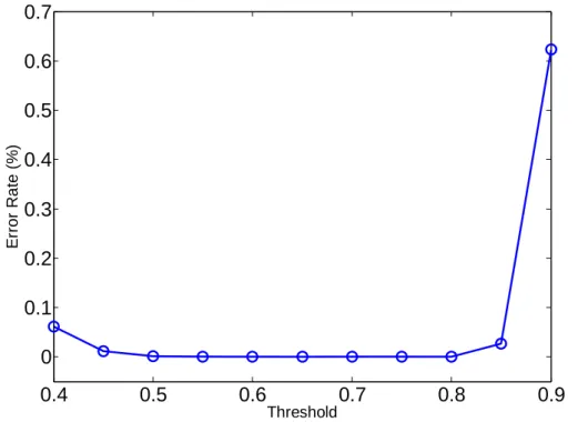
Fig. 3.7 illustrates the error rate under different threshold of the proposed mode/GI detection. The simulation environment is 1000 2K transmission mode symbols with 1/4 guard interval, 12dB SNR, 23.33 sub-carriers CFO and surviving from Rayleigh channel. As the simulation shows, the error rate of the proposed mode/GI detection method under the threshold 0.5 to 0.8 is zero. That means the pre-defined threshold value 0.707 locates at the reliable region. Because of noise and channel effect, the normalized correlation results are closing to 0.9 instead of 1. Therefore, the reliability decreases while the threshold is defined close to 0.9. For threshold smaller then 0.5 cases, the noise will influence the detection result.

0.4 0.5 0.6 0.7 0.8 0.9 0 0.1 0.2 0.3 0.4 0.5 0.6 0.7 E rror R a te (% ) Threshold

Fig. 3.7 Error rate under different threshold of proposed mode/GI detection

3.2 Coarse Symbol Synchronization

Coarse symbol synchronization (CSS) is also named symbol boundary detection. The goal of symbol boundary detection is to find out boundaries of transmitted symbols. Coarse symbol synchronization starts to work after finishing the mode/GI detection. With the information of transmission mode and guard interval length, symbol boundary detection has enough information to detect boundaries. After the first symbol boundary is detected, the system will use transmission mode, guard interval length and boundary location to derive the successive symbol boundaries.

In order to make the FFT windows locate on correct locations, symbol boundary detection needs to solve some problems. Since DVB-T signals are transmitted in SFN (Single Frequency Network), for a receiver there will have many signals from different transmitters with discordant delay time as Fig. 3.8 illustrates. The multipath effect leads to the same symbol with different delays overlaps and hard to detect the correct boundary of main path. Channel noises also reduce the reliability of coarse

symbol synchronization algorithms. The solution will be discussed in section.

≈≈

≈

≈

Fig. 3.8 Effect of multipath fading

3.2.1 Effect of Symbol Timing Offset

Before starting to introduce to coarse symbol synchronization algorithms, the effect of symbol timing offset must been derived. Symbol timing offset means the detected boundary does not locate on the true symbol boundary. This phenomenon is due to multipath effect, channel noise and aliasing. Two possible cases will occur, later or earlier than the true symbol boundary. Thanks to cyclic prefix, an earlier boundary location only causes a phase rotation which is able to be compensated by frequency domain equalization. The effect of the offset is derived in Eqn. (3.5).

N k j N n N k j N n k j N n N k j N n k j n N k j N N n k j N n N n k j n N n k j N n N n k j e k X e e n x e e n x e e N n x e n x e n x e n x k X k X ε π ε π π ε ε π ε π ε _π ε _π ε ε π ε _π π ε ε ε ε ε ε 2 1 0 2 2 1 _{2 2} 1 0 2 2 1 ₂ 1 0 2 1 0 2 ) ( ) ( ) ( ) ( ) ( ) ( ) ( ) ( ) ( ˆ = = − + − + = − + − = − = − =

∑

∑

∑

∑

∑

∑

− = − = − − = − + − = − = − = (3.5)

The case of earlier offset only leads to a phase rotation. But the derivation above only works whenεis not too large to make FFT window locates on ISI region. Otherwise, just like the later case, FFT window will get signals from previous symbol which has no orthogonality with the current symbol. Fig. 3.9 represents the sub-carriers after FFT by early and late cases in constellation map. The early case leads to a phase rotation in constellation map while the late case leads to mix-up in constellation map.

-2 -1.5 -1 -0.5 0 0.5 1 1.5 2 -2 -1.5 -1 -0.5 0 0.5 1 1.5 2 IM (z ) Re(z) (a) -2 -1.5 -1 -0.5 0 0.5 1 1.5 2 -2 -1.5 -1 -0.5 0 0.5 1 1.5 2 IM( z ) Re(z) (b)

3.2.2 Coarse Symbol Synchronization Algorithms

Coarse symbol synchronization aims at finding a rough symbol boundary. As a result of DVB-T system uses broadcasting technique to transmit signals in air, maximum-likelihood algorithms are not suit for DVB-T. Thanks to cyclic prefix again, like mode/GI detection, many coarse symbol synchronization algorithms are based on using the correlations between guard interval and symbol’s tail. There are three common algorithms, which are maximum correlation (MC) [19], normalized maximum correlation (NMC) [17] and minimum mean square error (MMSE) in [20]. In the following will compare their performance.

a) Maximum Correlation (MC) ) ( ) ( max arg 1 0 * _{n i r n i N} r K g N i n est=

∑

− × − − − = (3.6) Similar to mode/GI detection, maximum correlation algorithm uses guard interval length detected by mode/GI detection as Ng to detect the maximum peak

value. Unlike mode/GI detection, there will only be a maximum peak exist in stead of a plateau. Ideally, when the moving sum window goes into guard interval region, correlation will start to grow up. When the moving sum window exactly fits the whole guard interval region, a maximum peak occurs. Correlation value will decrease when the moving sum window start to leave the guard interval region.

b) Normalized Maximum Correlation (NMC)

) ( ) ( ) ( ) ( max arg ₁ 0 * 1 0 * i n r i n r N i n r i n r K g g N i N i n est − × − − − × − =

∑

∑

− = − = (3.7)

Normalized maximum correlation algorithm is similar to maximum correlation algorithm. By dividing its own power term, the peak is normalized to “1” ideally. A normalized peak makes the threshold easy to define and that’s why the modified normalized maximum correlation is adopted as mode/GI detection algorithm. But a penalty of an extra moving sum delay-line for power term and a divider are the disadvantages.

c) Minimum Mean Square Error (MMSE)

(

)

_⎟⎟ ⎠ ⎞ ⎜ ⎜ ⎝ ⎛ − − + − − − − × − =

∑

∑

− = − = 1 0 2 2 1 0 * _{( ) ( )} 2 1 ) ( ) ( max arg g g N i N i n est r n i r n i N r n i r n i N K (3.8)

This algorithm is similar to ML algorithm in [21], but the received signals replace the look-up table. It also likes a change of normalized maximum correlation algorithm. Since the maximum value of NMC is close to “1”, that means the numerator substrates the denominator will close to “0”. The characteristic of plateau, which is close to “0”, also can be used in mode/GI detection. But without a normalized threshold, MMSE is hard to tell from the plateau of 8K mode from bottom of other modes. As shown in Fig. 3.10 (a) and (b), the plateau value of 8K mode is closed to the bottom of 2K mode. Fig. 3.11 (a) and (b) show the boundary detection results of MMSE algorithm and the peak characteristic is similar to MC and NMC. The patterns of Fig. 3.10 and Fig. 3.11 are the same with Fig. 3.3.

0 1000 2000 3000 4000 5000 -9 -8 -7 -6 -5 -4 -3 -2 -1 0 Sample Index A m pl it ud e 2K MMSE 8K MMSE 2K MMSE 8K MMSE 0 0.5 1 1.5 2 x 104 -60 -50 -40 -30 -20 -10 0 Sample Index A m pl it ud e 2K MMSE 8K MMSE _{8K MMSE} 2K MMSE (a) (b) Fig. 3.10 MMSE mode/GI detection under (a) 2K (b) 8K mode

0 1000 2000 3000 4000 5000 -60 -50 -40 -30 -20 -10 0 Sample Index A m pl it ud e 2K MMSE 8K MMSE 2K MMSE 8K MMSE 0 0.5 1 1.5 2 x 104 -250 -200 -150 -100 -50 0 Sample Index A m pl it ud e 2K MMSE 8K MMSE 8K MMSE 2K MMSE (a) (b) Fig. 3.11 MMSE boundary detection under (a) 2K (b) 8K mode

As a result, NMC is adopted as mode/GI detection algorithm in this thesis because of the normalized plateau characteristic.

3.2.3 Performance Simulation and Comparisons

a) Accuracy Simulation

The symbol boundary location accuracy of MC, NMC and MMSE is simulated to compare the performance. The transmitted 1000 symbols will survive from two kinds of channels, Rayleigh and Ricean, with CFO equals to 23.33 sub-carriers, 2K transmission mode, 1/4 guard interval length, 50Hz Doppler spread and 12dB SNR. As Fig. 3.12, Fig. 3.13 and Table 3-1 shows, MMSE owns the best accuracy. The accuracy of MC and NMC are closely.

-150 -10 -5 0 5 10 15 20 5 10 15 20 25 30 35 P e rc e n ta ge (%)

Boundary Offset (Samples)

-150 -10 -5 0 5 10 15 20 5 10 15 20 25 30 35 P e rc e n ta ge (%)

Boundary Offset (Samples)

(a) (b) -150 -10 -5 0 5 10 15 20 5 10 15 20 25 30 35 40 45 P er c ent ag e ( % )

Boundary Offset (Samples)

(c)

Fig. 3.12 (a) MC, (b) NMC and (c) MMSE boundary offset distribution @ Ricean

-10 0 10 20 30 40 0 1 2 3 4 5 6 7 8 9 P er c ent ag e ( % )

Boundary Offset (Samples)

-10 0 10 20 30 40 0 1 2 3 4 5 6 7 8 P er c ent ag e ( % )

Boundary Offset (Samples)

-10 0 10 20 30 40 0 1 2 3 4 5 6 7 8 9 P er c ent ag e ( % )

Boundary Offset (Samples)

(c)

Fig. 3.13 (a) MC, (b) NMC and (c) MMSE boundary offset distribution @ Rayleigh Table 3-1 MC, NMC and MMSE boundary average/peak offset @ Ricean/Rayleigh

Name MC (Average/Peak Offsets) NMC (Average/Peak Offsets) MMSE (Average/Peak Offsets) Ricean 0.8051/18 0.7768/11 0.6020/7 Rayleigh 11.7687/36 11.4111/41 10.8273/29 b) Hardware Complexity

For 2K/4K/8K applications in DVB-T/H, all of the algorithms above must have at least an 8K long correlation delay-line, which is used to store the r(n-8K) signal and also can be used to store r(n-2K) and r(n-4K) signals, and a 2K (a quarter of 8K) long moving sum delay-line, which is used to integrate the 2K moving sum correlation values for 8K mode with 1/4 GI length, as Fig. 3.14 illustrates. Due to the correlation expression, a complex multiplier is necessary. Then two pairs of adders and subtractors, one for real part and another for image part, are used to do moving sum calculation. Finally, an additional complex multiplier is required to do the square operation. For NMC, an extra 2K moving sum delay-line, complex multiplier, adder and subtractor are needed for its power term denominator. The square operation of power term only needs a multiplier as a result of the power term is integer. Further more, a divider is needed for normalization operation. MMSE needs an extra complex

multiplier and adder comparing to the NMC denominator components and the divider is replaced by a subtractor. In summary, Table 3-2 lists the components required.

(a)

(b)

(c)

Fig. 3.14 Block diagram of (a) MC (b) NMC and (c) MMSE Table 3-2 Components required for MC, NMC and MMSE

Name Correlation/Moving Sum

Delay-Line Complex Multiplier Adder/ Subtractor Multiplier/ Divider MC 8K/2K 2 2/2 0/0 NMC 8K/2K×2 3 3/3 1/1 MMSE 8K/2K×2 4 4/4 1/0

The reason why MC is adopted as symbol boundary detection algorithm in this thesis is because of the performance is not differ too much to NMC and MMSE, but it needs the fewest components and no divider.

3.2.4 Proposed Mode/GI and Symbol Boundary Detection Scheme

By observing the mode/GI and boundary detection expression, it is easy to find out their structures are very similar. The mode/GI detection block diagram is illustrated in Fig. 3.15. The architecture is modified from NMC architecture by using the subtraction to replace the division as Eqn. (3.4) derived. As a result, mode/GI and boundary detection is able to share the same hardware to detect mode/GI and symbol boundary by controlling the correlation and moving sum delay-line lengths. After mode/GI detection, controller changes the correlation and moving sum delay-line lengths for symbol boundary detection.

Fig. 3.15 Block diagram of mode/GI detection

Fig. 3.16 illustrates the proposed mode/GI and boundary detection hybrid architecture. In the correlation part, the functions of 2K, 4K and 8K delays for different transmission modes are realized by a 2K/4K/8K triple modes reconfigurable delay-line and defined as correlation delay-line in this architecture. For four guard interval lengths of three transmission modes, there are totally six possible moving sum lengths and realized by two 2K/1K/512/256/128/64 reconfigurable delay-line, which is also named the moving sum (MS) delay-line.

Correlator [ ]* FFT Gate Gate D | |2 r(n) Moving Sum 2K/4K/8K delay 2K/1K/512/256 /128/64 delay MC2 Threshold to FCFO × × D CSS Controller FFT Out | |2 2K/1K/512/256 /128/64 delay

Fig. 3.16 Architecture of mode/GI and boundary detection scheme

The proposed mode/GI and CSS scheme can be divided into three stages, the first stage is mode detection, the second stage is guard interval length calculation and the final stage symbol is boundary detection. As Fig. 3.17 shows, the system first starts to detect the mode beginning from 2K then 4K and finally 8K mode. It spends 2K samples to fill the correlation delay-line and 64 samples (the minimum guard interval length of 2K) to fill the moving sum delay-line and then enter the 2K mode detection. The purpose to choose 2K mode as the first detected mode is it only needs 2K samples latencies to fill the correlation delay-line since others candidates need 4K or 8K samples. By using the twister memory access method based delay-line design to overlap the filling time and the previous mode detection time, the correlation delay-line does not have to refill or replenish when the detection mode is changed. As a result, the latency of the proposed scheme is reduced to only 2K samples.

Fig. 3.17 Finite state machine of mode/GI and boundary detection scheme The pseudo code of the proposed scheme is shown below.

1. Set the detection mode as 2K and fill the correlation delay-line with 2K samples.

2. Fill the moving sum with detection mode/32 samples. If the moving sum is filled and threshold=0, go to Step 3.

3. Detect the detection mode for a pre-defined detection period. If the threshold=1, jump to Step 4. Else if the detection counter=detection period,

jump to Step 2 and set the detection mode as detection mode×2.

4. Count the period length of threshold=1. If the threshold=0, set moving sum length as detected GI length and go to Step 5.

5. Fill the moving sum then find the maximum correlation result as boundary. 6. Derive the next boundaries using the detected mode, GI length and boundary.

After a detection period of (1+1/32)×2K ~ 2×(1+1/4)×2K samples, the system knows the transmission mode is not the same with 2K mode and then enters the “4K Dummy State” to do the 4K mode detection. Otherwise, if the threshold changes from low to high during the 2K mode detection period, it means the transmission mode is the 2K mode and so do other detection modes. The system jumps to “GI Detection State” as soon as the threshold turns to high and calculate the period length when it is high. The system period length is regarded as guard interval length. When the moving sum window accidentally locates on any place of the guard interval period initially, the threshold will turn to high before leaving “Dummy State”. This situation possibly

leads to an incorrect guard interval length. For the purpose to prevent this situation, the state won’t enter “Mode Detection State” before the threshold turns to low. Thus, the system only starts to calculate the guard interval length at the beginning of a plateau.

After mode/GI detection, the system enters the “Dummy Find Boundary State” and uses the detected guard interval length to refill the moving sum delay-line. After refilling the moving sum delay-line, the system has a best MC2 result. By observing the MC2 results during plateau, the location of the maximum MC2 result subtracts half of the guard interval length will be the rough symbol boundary. After all, the system predicts the successive boundaries using the detected mode, GI length and first boundary information.

The required time of the proposed scheme is analyzed below. For the 2K transmission mode, it needs 2K samples to fill correlation delay-line, 64 samples to fill moving sum delay-line, 1 ~ (1+1/32)×2K samples for mode detection, 64~512 samples for calculating guard interval length and (1+1/32)×2K ~ (1+1/4)×2K for boundary detection. Theoretically, 7296 samples is the worst case to finish the mode/GI and symbol boundary detection scheme. The system stays at “2K Mode Detection State” for at least (1+1/32) × 2K samples to guarantee the possible peak/plateau is detected. Without enough stay time, the detector is possible to miss the peak/plateau. After this, the system jumps to “4K Dummy State” and changes the correlation delay-line to 4K mode and refill the moving sum delay-line. While the mode changes to 4K, it’s not necessary to refill or replenish the correlation delay-line because of the signal r(n-4k) is already in the correlation delay-line. The other procedures are similar to 2K mode and so do 8K mode. Table 3-3 lists the required samples for different transmission modes.

Table 3-3 Timing for mode/GI and boundary detection

Mode Modedet_t GIdet_t Boundarydet_t Totaldet_t

2K 2K+64+(1~2K+64) 64~512 2K+2K_GIdet_t

2K_Modedet_t+2K_GIdet_t

+2K_Boundarydet_t

4K Max(2K_Modedet_t)

+128+(1~4K+128) 128~1K 4K+4K_GIdet_t

4K_Modedet_t+4K_GIdet_t

+4K_Boundarydet_t

8K Max(4K_Modedet_t)

+256+(1~8K+256) 256~2K 8K+8K_GIdet_t

8K_Modedet_t+8K_GIdet_t

+8K_Boundarydet_t

Comparing to parallel mode detection shown in Fig. 3.18 (a), (b) and (c), the proposed scheme, shown in Fig. 3.18 (f), has the same latency for 2K transmission mode and an extra delay depends on mode detection period for other modes. But only single hardware is necessary for different mode detection. For the sequential mode detection shown in Fig. 3.18 (d) and (e), the proposed scheme saves 12K sample as a result of using twister memory access based delay-line. In summary, only 384 samples (2.27%) more than parallel 8K mode detection, 12K samples (41.56%) less than sequential mode detection (refill) and 6K samples (26.23%) less than sequential mode detection (replenish).

Delay-Line Filling Moving Sum

Delay-Line Filling (a) t 2K Mode Detection 4K Mode Detection 8K Mode Detection (d) (f) (b) (c) (e) 2K, 64, 2K+64 (4224) 4K, 128, 4K+128 (8448) 8K, 256, 8K+256 (16896) 2K, 64, 2K+64, 4K, 128, 4K+128, 8K, 256, 8K+256 (29568) 2K, 64, 2K+64, 2K, 128, 4K+128, 4K, 256, 8K+256 (23424) 2K, 64, 2K+64, 128, 4K+128, 256, 8K+256 (17280)

Fig. 3.18 Timing of parallel (a) 2K, (b) 4K, (c) 8K, sequential (d) refill, (e) replenish and (f) proposed mode detection schemes

Fig. 3.19 (a), (b), (c) and (d) show the simulation result of the proposed scheme for 2K and 8K transmission modes in MC2 and NMC using the same pattern with Fig. 3.3. The aliasing peak is caused by the moving sum doesn’t accumulate enough values

and it only occurs at “Dummy States”. As Fig. 3.19 shows, without the assistance of NMC, the correlation values during GI detection period is much smaller than the boundary detection period and the system is not easy to define the GI detection period. With the assistance of NMC, to define the GI detection period and compute the period length becomes much easier for the system. Furthermore, for the purpose to improve the reliability, the threshold detector is realized using 8 states confidence counter. The simulation environment is 2K/8K transmission symbols with 1/4 GI, 23.33 CFO, 12dB SNR and surviving from Rayleigh channel.

0 1000 2000 3000 4000 5000 6000 7000 0 500 1000 1500 2000 2500 A m p lit u d e Sample Index 2K Filling 2K Mode Detection GI Detection Boundary 0 1000 2000 3000 4000 5000 6000 7000 0 0.2 0.4 0.6 0.8 1 A m p lit u d e Sample Index 2K Filling Aliasing Peak GI Detection Boundary (a) (b) 0 0.5 1 1.5 2 x 104 0 0.5 1 1.5 2 2.5 3 3.5 4 4.5x 10 4 A m p lit u d e Sample Index 2K Filling 2K/8K Mode Detection GI Detection Boundary 0 0.5 1 1.5 2 x 104 0 0.2 0.4 0.6 0.8 1 A m p lit u d e Sample Index 2K Filling

Aliasing Peak Aliasing Peak

2K/8K Mode Detection GI Detection

Boundary Aliasing Peak

(c) (d) Fig. 3.19 (a) 2K MC2, (b) 2K NMC, (c) 8K MC2 and (d) 8K NMC simulation of the

proposed blind mode/GI boundary detection scheme

In summary, an efficient sequential mode/GI and boundary detection scheme using normalized plateau to compute the guard interval length with single hardware, which is also used by boundary detection, is proposed in this chapter.

Chapter 4

Channel Estimation Algorithms

This chapter will focus on channel estimation issued. First, the scattered pilot synchronization (SPS), which is also called scattered pilot mode detection, will be discussed for the purpose to extract the correct scattered pilots for channel estimation. After the scattered pilot mode is detected, the channel estimation collects the scattered pilots and using their value to estimate the channel response. Finally, a division-free equalizer and three-stage demapping hybrid architecture will be described.

4.1 Scattered Pilot Synchronization

The inserted scattered pilots are useful for the purpose to estimate the channel response for channel estimation. Unfortunately, unlike the continuous pilots, the distribution of scattered pilots is not fixed with regular locations. As Eqn. (2.2) shows, there are four scattered pilot distribution modes. Typically, the scattered pilot distribution can be known after TPS synchronization. But it takes 17~68 symbols to decode the TPS pilots and it spends too many time. For DVB-H application, the synchronization time is strictly limited. Therefore, using fast scattered pilot synchronization technique to accelerate the synchronization timing is necessary. This section will introduce two fast scattered pilot detection algorithms. Performance simulation and hardware complexity comparison is carried out. Furthermore, an idea of two-stage scattered pilot synchronization scheme with extracted scattered pilots pre-filling, which is required by channel estimation to estimate the channel response, will be described.

4.1.1 Fast Scattered Pilot Synchronization Algorithms

In order to detect the scattered pilot distribution mode as soon as possible, two fast scattered pilot synchronization algorithms were proposed in [22] [23] and will be discussed below.

a) Power-Based Scattered Pilots Mode Detection

The first algorithm is power-based scattered pilot mode detection algorithm (PB) as shown in Eqn. (4.1):

{

1,2,3,4

}

)); ( max( ) 9 12 , ( ) 9 12 , ( ) ( ) 6 12 , ( ) 6 12 , ( ) ( ) 3 12 , ( ) 3 12 , ( ) ( ) 12 12 , ( ) 12 12 , ( ) ( * 0 4 * 0 3 * 0 2 * 0 1 max max max max ∈ = + ⋅ + = + ⋅ + = + ⋅ + = + ⋅ + =

∑

∑

∑

∑

= = = = p n PS Mode Pilot Scattered p n SC p n SC n PS p n SC p n SC n PS p n SC p n SC n PS p n SC p n SC n PS P p p p p p p p p (4.1)

where pmax is 141 for 2K, 283 for 4K and 567 for 8K mode, SC(n,m) is the mth

sub-carrier of the nth OFDM symbol. The power-based algorithm uses the

characteristic of scattered pilots’ boosted power by 4/3. It’s easy to see that only the correct scattered pilots have the largest `power due to its boosted power. By observing the power accumulation of four possible scattered pilot distributions, the scattered pilot mode can be detected.

b) Correlation-Based Scattered Pilots Mode Detection

The second algorithm is correlation-based scattered pilot mode detection algorithm (CB). By using the similar skill as Eqn. (4.1) but multiplying the same

sub-carriers located four OFDM symbols before instead of itself. This method is stronger to against noise. But if Doppler effect changes the channel response significantly after four symbols time, the performance of this algorithm will be affected by Doppler effects. Eqn. (4.2) presents the correlation-based scattered pilot mode detection algorithms mathematically.

{

1,2,3,4

}

)); ( max( ) 9 12 , 4 ( ) 9 12 , ( ) ( ) 6 12 , 4 ( ) 6 12 , ( ) ( ) 3 12 , 4 ( ) 3 12 , ( ) ( ) 12 12 , 4 ( ) 12 12 , ( ) ( * 0 4 * 0 3 * 0 2 * 0 1 max max max max ∈ = + − ⋅ + = + − ⋅ + = + − ⋅ + = + − ⋅ + =

∑

∑

∑

∑

= = = = p n CS Mode Pilot Scattered p n SC p n SC n CS p n SC p n SC n CS p n SC p n SC n CS p n SC p n SC n CS P p p p p p p p p (4.2)

Comparing to the second method, the first one is better in against Doppler Effects and doesn’t require a latency of four symbols due to multiplying sub-carriers itself. This implies that the power-based algorithm is four symbols time faster than the correlation-based and requires no sub-carriers storage memory to save the scattered pilots of four distributions four symbols before current symbol. Though the scattered pilot storage can be done by using the channel estimation storage memories and does not cause an additional hardware overhead, the ability to against Doppler effects and fast to get the result makes power-based scattered pilot mode detection algorithm the choice in scattered pilot mode detection.

4.1.2 Performance Simulation and Comparisons

Fig. 4.1 shows the error rate of the above two algorithms under different Signal-to-Noise Ratio (SNR). The environment is 1000 2K transmission mode symbols with 1/4 guard interval length, Rayleigh channel, 10 samples earlier than correct boundary. The residual CFOs after fractional and integer CFO compensation are (a) zero (b) 0.03 sub-carrier and (c) 0.33 sub-carrier. As shown in Fig. 4.1, the error rate of power-based algorithm starts to increase when SNR below 2dB and the correlation based algorithm starts to increase when the SNR below -6dB. Generally, as [1] defined, the SNR is bigger than 3 dB and the accidentally scattered pilot mode detection error is only need to be concerned.

-21 -18 -15 -12 -9 -6 -3 0 3 6 10-1 100 101 102 SNR (dB) E rror R a te (% ) Power-Based Correlation-Based (a) -21 -18 -15 -12 -9 -6 -3 0 3 6 10-1 100 101 102 SNR (dB) E rro r R a te ( % ) Power-Based Correlation-Based -21 -18 -15 -12 -9 -6 -3 0 3 6 9 12 10-1 100 101 102 SNR (dB) E rr o r R a te (% ) Power-Based Correlation-Based (b) (c) Fig. 4.1 Error rate of two SPS algorithms versus SNR with (a) 0 (b) 0.03 (c) 0.33 CFO