在PACDSP平台上之MPEG-4視訊解碼器軟體實現

全文

(1)國. 立. 交. 通. 大. 學. 電子工程學系電子研究所碩士班碩. 士. 論. 文. 在 PACDSP 平台上之 MPEG-4 視訊解碼器軟體實現. Software Implementation of MPEG-4 Video Decoder on PACDSP Platform. 研究生 : 蔡崇諺指導教授 : 林大衛博士中華民國九十五年六月.

(2) 在 PACDSP 平台上之 MPEG-4 視訊解碼器軟體實現. Software Implementation of MPEG-4 Video Decoder on PACDSP Platform. 研究生 : 蔡崇諺指導教授 : 林大衛博士. Student : Chung-Yen Tsai Advisor : Dr. David W. Lin. 國立交通大學電子工程學系電子研究所碩士班碩士論文 A Thesis Submitted to Department of Electronics Engineering & Institute of Electronics College of Electrical and Computer Engineering National Chiao Tung University In Partial Fulfillment of the Requirements For the Degree of Master of Science In Electronics Engineering June 2006 Hsinchu, Taiwan, Republic of China. 中華民國九十五年六月.

(3) 在 PACDSP 平台上之 MPEG-4 視訊解碼器軟體實現. 研究生: 蔡崇諺. 指導教授:林大衛博士. 國立交通大學電子工程學系. 電子研究所碩士班. 摘要. MPEG-4 為一廣泛應用之多媒體訊號壓縮標準。本篇論文介紹在 PACDSP 平台上 MPEG-4 視訊解碼器之實現，本平台由一超長指令數位訊號處理器與一 ARM920T 處理器所組成。為了最佳化程式流程，我們也完成了許多的靜態分析，並且利用超長指令處理器架構上之特性來達到即時解碼。我們也完成了簡單的雙核心展示並驗證其正確性。在我們的實作當中，我們使用了 MPEG-4 參考軟體，MoMuSys，當作驗證的比較對象。首先，我們分析了 MPEG-4 基於圖像解碼器之運算複雜度並藉此找到有效率的實現方法。接著，我們根據離散餘弦轉換（DCT）之特性來跳過多餘的運算，並且對於全零之剩餘方塊亦有許多可略過之計算。為了加速執行時間，我們將規律之運算分佈於兩組以增加處理器之效能。我們也使用單指令多資料（SIMD）指令以及一般指令層級平行化來減少處理器之延遲。我們討論了離散餘弦反轉換（IDCT）之效能與精確度，並且我們的實現能夠符合 IEEE1180-1190 標準之規範。我們所使用之演算法在效能上也具有與其他實現競爭的能力。在所有的最佳化之後，我們在最差情況下解碼一張 QCIF 格式之圖像需要 5,700,000.

(4) 週期。也就是說，對一個工作在 175MHz 的真實 PACDSP 晶片而言，我們能夠達到每秒三十張畫面之即時解碼。而整個程式的大小為 27 Kbytes，也小於 PACDSP 的程式快取記憶體大小 32 Kbytes。最後我們在 PSDK 平台上展示了雙核心的實現。在本篇論文當中，我們首先介紹了 MPEG-4 標準以及 PADSP 平台之概述。接著討論靜態分析、實作策略、最佳化方法、以及實驗結果。最後簡單介紹了展示雙核心實現的系統與機制。.

(5) Software Implementation of MPEG-4 Video Decoder on PACDSP Platform. Student: Chung-Yen Tsai. Advisor: Dr. David W. Lin. Department of Electronics Engineering Institute of Electronics National Chiao Tung University. Abstract MPEG-4 is a widely-applied multimedia coding standard. This thesis presents an implementation of MPEG-4 video decoder on the PACDSP platform, which consists of a VLIW digital signal processor (DSP) and an ARM920T processor. We complete many anlyses to optimize the program flow and utilize the advantage of VLIW processor to achieve real-time decoding. A simple dual-core demostration is completed and verified. In our implementation, the MPEG-4 reference software, MoMuSys, is used as a golden model to verily our implementation. First, we analyze the computational complexity of the MPEG-4 frame-based video decoder, and find efficient algorithms for the implementation. Second, we skip some computations according to the nature of discrete cosine transform (DCT), and there are also lots of comutation skipped for all-zero residual blocks. Third, to speed up the execution time, we distribute the regular computations to both clusters to increase the efficiency of the processor. Single-instruction-multiple-data (SIMD) instructions and general instruction level parallelism also utilized to reduce the processor stalls. We also discuss the efficiency.

(6) and accuracy of IDCT, and the accuracy of our IDCT implementation can meet the IEEE 1180-1190 standard. The performance of our alogorithm is also competitive to other implementations. After all the optimizations, the worst-case computaion time for QCIF format is less than 5,700,000 cycles. That is, our implementation can achieve real-time decoding, 30 frame-per-second, for a real PACDSP chip running over 175 MHz. The code size is 27 Kbyte, which is smaller than the 32-Kbyte instruction cache on PACDSP. Finally, we demonstrate a simple dual-core implementation on the PAC System Developer’s Kit (PSDK). In this thesis, we first introduce the MPEG-4 standard and give an overview of the PACDSP platform. Then the static analysis, implementation strategies, the optimiztion methods, and the experiment results are discussed. Finally, we brief the system and mechanism for demonstration of the dual-core implementation on PSDK plarform..

(7) 誌謝. 本篇論文的完成，誠摯地感謝我的指導老師林大衛博士，從電控系推甄進入電子所這個新環境時，多虧老師的循循善誘，不論在課業、研究、或者心理上遭遇挫折時的鼓勵與指導而能夠一次一次地解決困難，並且讓我學習了分析問題並加以解決的能力。而老師身體力行與樂觀積極的生活態度也深深地影響了我。在此，僅向老師及老師的家人致上最高的感謝之意。. 感謝在電子研究所 CommLab 的日子裡實驗室所提供完善的研究資源。承蒙崑健、家揚、俊榮、朝雄等學長的提攜與照顧，在研究與生活上都能夠順利解決問題。而實驗室的同伴，鴻志、和璋、家賢、治傑、韋霖、旻弘、育彰、宗熹、德亘，以及室友浩緯、人中等在課業上的砥礪與生活上的幫助也讓我在忙碌的研究所生涯中仍舊擁有快樂的心情。此外，也要感謝學弟，政達、介遠，在你們的討論與幫助下，研究才能夠更加迅速與正確地完成。. 最後，感謝我的家人，溫暖的家一直是我求學生涯中最強而有力的後盾，感謝你們的努力讓我能夠無後顧之憂地汲取知識，繼續升學。另外感謝我的女友，楊晨，在我求學過程一路相伴，面對壓力時不斷地鼓勵。僅將本論文獻給我敬愛的父母，蔡文彬先生、王阿珠女士，以及我摯愛的楊晨小姐。. 蔡崇諺二００六年六月于新竹.

(8) Contents 1. Introduction. 1. 2. Overview of the MPEG-4 Video Standard. 3. 2.1. Structure of MPEG-4 Video Data . . . . . . . . . . . . . . . . . . . . . .. 3. 2.2. MPEG-4 Video Texture Coding . . . . . . . . . . . . . . . . . . . . . .. 6. 2.3. Motion Coder . . . . . . . . . . . . . . . . . . . . . . . . . . . . . . . .. 6. 2.4 3. 2.3.1. Texture Coder . . . . . . . . . . . . . . . . . . . . . . . . . . . .. 10. 2.3.2. Other Video Coding Tools [3] . . . . . . . . . . . . . . . . . . .. 15. 2.3.3. Robust Video Coding . . . . . . . . . . . . . . . . . . . . . . . .. 15. 2.3.4. Scalable Coding . . . . . . . . . . . . . . . . . . . . . . . . . .. 16. Profiles and Levels [2] . . . . . . . . . . . . . . . . . . . . . . . . . . .. 16. Overview of The PACDSP. 19. 3.1. Introduction . . . . . . . . . . . . . . . . . . . . . . . . . . . . . . . . .. 19. 3.1.1. Architecture Features . . . . . . . . . . . . . . . . . . . . . . . .. 20. 3.2. Architecture Overview . . . . . . . . . . . . . . . . . . . . . . . . . . .. 21. 3.3. Program Sequence Control Unit . . . . . . . . . . . . . . . . . . . . . .. 22. 3.3.1. Branch Instruction . . . . . . . . . . . . . . . . . . . . . . . . .. 22. 3.3.2. Loop . . . . . . . . . . . . . . . . . . . . . . . . . . . . . . . .. 23. 3.3.3. Customized Function Unit (CFU) . . . . . . . . . . . . . . . . .. 24. 3.3.4. Exception Handling . . . . . . . . . . . . . . . . . . . . . . . .. 24. 3.3.5. Interrupt Handling . . . . . . . . . . . . . . . . . . . . . . . . .. 24. VLIW Datapath . . . . . . . . . . . . . . . . . . . . . . . . . . . . . . .. 25. 3.4. I.

(9) 3.4.1. Ping-Pong Register File . . . . . . . . . . . . . . . . . . . . . .. 25. 3.4.2. Data/Address/Accumulator Registers . . . . . . . . . . . . . . .. 25. 3.4.3. Status and Control Registers . . . . . . . . . . . . . . . . . . . .. 26. 3.4.4. Addressing Modes . . . . . . . . . . . . . . . . . . . . . . . . .. 28. 3.4.5. VLIW Datapath . . . . . . . . . . . . . . . . . . . . . . . . . . .. 30. 3.4.6. Data Exchange . . . . . . . . . . . . . . . . . . . . . . . . . . .. 31. 3.4.7. Constant Register File . . . . . . . . . . . . . . . . . . . . . . .. 33. Scalar Unit . . . . . . . . . . . . . . . . . . . . . . . . . . . . . . . . .. 34. 3.5.1. Overview . . . . . . . . . . . . . . . . . . . . . . . . . . . . . .. 34. 3.5.2. Control Registers . . . . . . . . . . . . . . . . . . . . . . . . . .. 34. 3.5.3. General Purpose Scalar Register File . . . . . . . . . . . . . . .. 35. 3.6. Conditional Execution Control . . . . . . . . . . . . . . . . . . . . . . .. 36. 3.7. ISA and Pipeline Stages . . . . . . . . . . . . . . . . . . . . . . . . . . .. 37. 3.8. DSP Running Modes . . . . . . . . . . . . . . . . . . . . . . . . . . . .. 38. 3.9. Instruction Packet . . . . . . . . . . . . . . . . . . . . . . . . . . . . . .. 39. 3.10 Development Tools and Implementation Considerations . . . . . . . . . .. 39. 3.10.1 Development Tools . . . . . . . . . . . . . . . . . . . . . . . . .. 39. 3.10.2 Implementation Considerations . . . . . . . . . . . . . . . . . .. 42. 3.5. 4. Complexity Analysis and Implementation Strategy of MPEG-4 Framed-Based Video Decoder. 43. 4.1. Profiles of The MPEG-4 Frame-Based Video Decoder . . . . . . . . . . .. 44. 4.1.1. Approach to Complexity Analysis . . . . . . . . . . . . . . . . .. 44. 4.1.2. Profile on PC Using Intel VTune Performance Analyzer . . . . .. 45. 4.1.3. Low-Level Computational Analysis . . . . . . . . . . . . . . . .. 46. Implementation Strategies on PACDSP . . . . . . . . . . . . . . . . . . .. 49. 4.2.1. Efficient Variable Length Decoding (VLD) . . . . . . . . . . . .. 50. 4.2.2. Efficient Motion Compensation . . . . . . . . . . . . . . . . . .. 55. 4.2.3. Profile on PACDSP of All Decoder Functions . . . . . . . . . . .. 56. 4.2. II.

(10) 5. Optimization of The Implementation on PACDSP. 61. 5.1. Algorithmic Optimization . . . . . . . . . . . . . . . . . . . . . . . . . .. 61. 5.1.1. Algorithmic Optimization for Intra Frames . . . . . . . . . . . .. 61. 5.1.2. Algorithmic Optimization for P-Frames . . . . . . . . . . . . . .. 65. Architectural Optimization . . . . . . . . . . . . . . . . . . . . . . . . .. 67. 5.2.1. General Optimization Techniques . . . . . . . . . . . . . . . . .. 68. 5.2.2. Advantages of PACDSP . . . . . . . . . . . . . . . . . . . . . .. 71. Experiment Results . . . . . . . . . . . . . . . . . . . . . . . . . . . . .. 72. 5.3.1. Optimization of Dequantization . . . . . . . . . . . . . . . . . .. 72. 5.3.2. Implementation of IDCT . . . . . . . . . . . . . . . . . . . . . .. 73. 5.3.3. Overall Optimization of the implementation . . . . . . . . . . . .. 79. 5.4. Conclusion on Optimization . . . . . . . . . . . . . . . . . . . . . . . .. 80. 5.5. The Effect of Different Quantization Step (QP) . . . . . . . . . . . . . .. 81. 5.5.1. Effects of QP to I-Frame Decoding . . . . . . . . . . . . . . . .. 82. 5.5.2. Effects of QP to P-Frame Decoding . . . . . . . . . . . . . . . .. 83. Comparison with Other Implementations . . . . . . . . . . . . . . . . . .. 84. 5.2. 5.3. 5.6 6. Conclusion and Future Work. 89. 6.1. Conclusion . . . . . . . . . . . . . . . . . . . . . . . . . . . . . . . . .. 89. 6.2. Future Work . . . . . . . . . . . . . . . . . . . . . . . . . . . . . . . . .. 90. A Demonstration of MPEG-4 Frame-Based Video Decoder on Dual-Core PSDK 94 A.1 Overview of The PSDK 2.0 Platform . . . . . . . . . . . . . . . . . . . .. 94. A.2 Introduction to Dual-Core Demonstration . . . . . . . . . . . . . . . . .. 96. A.2.1 I-Frames Decoding . . . . . . . . . . . . . . . . . . . . . . . . .. 96. A.2.2 P-Frames Decoding . . . . . . . . . . . . . . . . . . . . . . . . .. 97. B C Program and Assembly Code of IDCT. 99. B.1 C Program of IDCT in MoMuSys . . . . . . . . . . . . . . . . . . . . .. 99. B.2 Original Assembly Code of IDCT . . . . . . . . . . . . . . . . . . . . .. 99. B.3 Optimized Assembly Code of IDCT . . . . . . . . . . . . . . . . . . . .. 99. III.

(11) List of Figures 2.1. Segmentation of a frame into VOPs (from [3]). . . . . . . . . . . . . . .. 4. 2.2. Structure of coded video data (from [4]). . . . . . . . . . . . . . . . . . .. 5. 2.3. Types of VOP. . . . . . . . . . . . . . . . . . . . . . . . . . . . . . . . .. 6. 2.4. Positions of luminance and chrominance samples in 4:2:0 data (from [5]).. 7. 2.5. Motion vector prediction (from [5]). . . . . . . . . . . . . . . . . . . . .. 9. 2.6. Quantizers in H.263. (a) For intra DC coefficient only. (b) For inter DC and all AC coefficients. . . . . . . . . . . . . . . . . . . . . . . . . . . .. 12. 2.7. Prediction of DC coefficients of blocks in an intra MB (from [3]). . . . .. 14. 2.8. Prediction of AC coefficients of blocks in an intra MB (from [3]). . . . .. 14. 2.9. Scans for 8 × 8 blocks (from [2]). . . . . . . . . . . . . . . . . . . . . .. 15. 3.1. Architecture of the PACDSP [1]. . . . . . . . . . . . . . . . . . . . . . .. 22. 3.2. Ping-pong register file in one cluster [1]. . . . . . . . . . . . . . . . . . .. 26. 3.3. The available registers in one cluster [1].. . . . . . . . . . . . . . . . . .. 27. 3.4. Illustration of the addressing mode control register (AMCR) [1]. . . . . .. 28. 3.5. Illustration of multiplication instructions with different precisions [1]. . .. 31. 3.6. Different load/store instructions [1]. . . . . . . . . . . . . . . . . . . . .. 32. 3.7. Data Exchange between Two Clusters [1]. . . . . . . . . . . . . . . . . .. 33. 3.8. Data broadcast among clusters [1]. . . . . . . . . . . . . . . . . . . . . .. 33. 3.9. The Constant Register File of one cluster [1]. . . . . . . . . . . . . . . .. 35. 3.10 PACDSP instruction set architecture [1]. . . . . . . . . . . . . . . . . . .. 38. 3.11 Pipeline stages of the PACDSP [1]. . . . . . . . . . . . . . . . . . . . . .. 38. 3.12 Transitions between DSP running modes [1]. . . . . . . . . . . . . . . .. 41. IV.

(12) 3.13 Syntax of instruction packet [1]. . . . . . . . . . . . . . . . . . . . . . .. 42. 3.14 Simplified syntax of instruction packet [1]. . . . . . . . . . . . . . . . . .. 42. 4.1. Block diagram of MPEG-4 frame-based video decoder [2]. . . . . . . . .. 44. 4.2. Example of bit by bit matching on PACDSP. . . . . . . . . . . . . . . . .. 53. 4.3. Example of one table mapping with magnitude-offset on PACDSP. . . . .. 54. 4.4. Example of multiple-pass matching on PACDSP. . . . . . . . . . . . . .. 55. 4.5. Example of bounded multiple-pass lookup with magnitude-offset on PACDSP. 56. 4.6. Comparison of different VLD methods on PACDSP . . . . . . . . . . . .. 57. 5.1. DC spreading from decoded coefficient to output block. . . . . . . . . . .. 62. 5.2. Assembly code of DC spreading. . . . . . . . . . . . . . . . . . . . . . .. 62. 5.3. Assembly code of new check in vertical AC reconstruction. . . . . . . . .. 65. 5.4. Example of vector addition. . . . . . . . . . . . . . . . . . . . . . . . . .. 69. 5.5. Example of static rescheduling technique. . . . . . . . . . . . . . . . . .. 70. 5.6. Example of loop unrolling technique. . . . . . . . . . . . . . . . . . . .. 70. 5.7. Example of software pipelining technique . . . . . . . . . . . . . . . . .. 71. 5.8. Original and optimized assembly code of IQ. . . . . . . . . . . . . . . .. 75. 5.9. The IDCT algorithm used in MoMuSys. . . . . . . . . . . . . . . . . . .. 78. 5.10 The even-odd decomposition IDCT algorithm[8]. . . . . . . . . . . . . .. 79. 5.11 Speed-up of different optimization methods for I-frames. . . . . . . . . .. 84. 5.12 Speed-up of different optimization methods for P-frames. . . . . . . . . .. 85. A.1 PAC System Developer’s Kit (PSDK) 2.0 . . . . . . . . . . . . . . . . .. 95. A.2 Memory map of the dualcore demonstration . . . . . . . . . . . . . . . .. 96. A.3 Co-processing mechanism for I-frames . . . . . . . . . . . . . . . . . . .. 97. A.4 Co-processing mechanism for P-frames . . . . . . . . . . . . . . . . . .. 98. B.1 C program of IDCT in MoMuSys reference software including clipping. . 100 B.2 Assembly code of our initial IDCT implementation (horizontal processing).101 B.3 Assembly code of our initial IDCT implementation (vertical processing and clipping). . . . . . . . . . . . . . . . . . . . . . . . . . . . . . . . . 102. V.

(13) B.4 Assembly code of optimized IDCT implementation (horizontal processing).103 B.5 Assembly code of optimized IDCT implementation (vertical processing and clipping). . . . . . . . . . . . . . . . . . . . . . . . . . . . . . . . . 104. VI.

(14) List of Tables 2.1. Weighting Values H0 (i, j), H1 (i, j), and H2 (i, j) . . . . . . . . . . . . .. 11. 2.2. Default Quantization Matrix (Q) [2] . . . . . . . . . . . . . . . . . . . .. 13. 2.3. Nonlinear Scaler for DC Coefficients (from [2]) . . . . . . . . . . . . . .. 13. 2.4. Profiles and Tools (from [2]) . . . . . . . . . . . . . . . . . . . . . . . .. 18. 3.1. Details of Control Register Files [1] . . . . . . . . . . . . . . . . . . . .. 36. 3.2. Memory-Mapped Control Registers [1] . . . . . . . . . . . . . . . . . .. 37. 3.3. Pipeline Stages and Their Descriptions. . . . . . . . . . . . . . . . . . .. 39. 3.4. Running Modes of the PACDSP [1] . . . . . . . . . . . . . . . . . . . .. 40. 3.5. Instruction Type in Each Instruction Slot. . . . . . . . . . . . . . . . . .. 41. 4.1. Profile of Frame-Based MPEG-4 Decoding of QCIF on PC . . . . . . . .. 46. 4.2. Complexity of Luminance Motion Compensation in One QCIF Frame . .. 48. 4.3. Complexity of Chrominance Motion Compensation in One QCIF Frame .. 49. 4.4. Complexity of Dequantization and IDCT for One 8×8 Block in MoMuSys Code . . . . . . . . . . . . . . . . . . . . . . . . . . . . . . . . .. 50. 4.5. Variable Length Codes for dct dc size luminance [2] . . . . . . . . . . .. 52. 4.6. Execution Time of Different VLD Methods on PACDSP . . . . . . . . .. 58. 4.7. Analysis of Necessary Interpolation Using MoMuSys . . . . . . . . . . .. 59. 4.8. Estimated Profile of Frame-Based MPEG-4 Decoding of QCIF on PACDSP 60. 5.1. Number of Skipped Blocks in 90 Intra Frames (Check CBP and ACPred Flag. Only) . . . . . . . . . . . . . . . . . . . . . . . . . . . . . . . . . . . .. VII. 64.

(15) 5.2. Number of Skipped Blocks in 90 Intra Frames with Further Check After AC Prediction . . . . . . . . . . . . . . . . . . . . . . . . . . . . . . . .. 66. 5.3. Execution Time of Intra Frame Decoding on PACDSP . . . . . . . . . . .. 66. 5.4. Number of Skipped Blocks in 89 P Frames . . . . . . . . . . . . . . . . .. 67. 5.5. Execution Time of Inter (P) Frame Decoding on PACDSP . . . . . . . . .. 68. 5.6. Analysis of Skipped Coefficients in Dequantization (90 I-frames) . . . . .. 74. 5.7. Improvement after Optimization of Dequatization . . . . . . . . . . . . .. 76. 5.8. Comparison of Computational Complexity for 8-point IDCT . . . . . . .. 76. 5.9. Test of Compliance Using IEEE Std. 1180-1190 . . . . . . . . . . . . . .. 77. 5.10 Comparison of IDCT on Different Platforms . . . . . . . . . . . . . . . .. 80. 5.11 Improvement After Optimization of IDCT . . . . . . . . . . . . . . . . .. 81. 5.12 Overall Optimization after IDCT Optimization . . . . . . . . . . . . . .. 82. 5.13 Execution Time Before and After Optimizations . . . . . . . . . . . . . .. 83. 5.14 Number of Skipped Blocks in 90 Intra Frames with Different QP. 86. . . . .. 5.15 Effects of Different QP to Execution Time of I-Frame Decoding on PACDSP 86 5.16 Number of Skipped Blocks in 89 P-Frames with Different QP . . . . . .. 87. 5.17 Percentage of Fractional Motion Vectors with Different QP . . . . . . . .. 87. 5.18 Effects of Different QP to Execution Time of P-Frame Decoding on PACDSP 88 5.19 Performance of MPEG-4 Video Decoder on Different Platforms . . . . .. VIII. 88.

(16) Chapter 1 Introduction In modern industry, compression of audio-visual information becomes more and more important, especially for applications on mobile devices. Besides, digital signal processors (DSPs) are also popularly used on these mobile devices. Our goal is the implementation of MPEG-4 video decoder on the PACDSP platform. The MPEG-4 standard for coding of audio-visual information has been widely adopted in various consumer products. There are several tools in the MPEG-4 standards, and they are used for different purposes. Since the present work is the first attempt to implement MPEG-4 video codecs on the PACDSP platform, we decide to implement the freme-based part of the MPEG-4 decoder first, and the corresponding encoder and other MPEG-4 video tools are left to the future work. PACDSP is a high performance, low cost VLIW (Very Long Instruction Word) DSP for multimedia applications[1]. Optimized architecture for data stream applications gives a strong reason for system designers to use PACDSP to implement media codecs. The instruction set architecture (ISA) of PACDSP is optimized for audio and video applications, so PACDSP is suitable for products with multi-standard codec requirement. In addition, the low power design for PACDSP makes it possible to use PACDSP on portable devices. This thesis is organized as follows. Chapter 2 is the overview of MPEG-4 standards. Chapter 3 introduces the architecture and specification of the PACDSP platform. Chapter 4 is the analysis of complexity for the reference software of MPEG-4. In addition, the implementation strategy of MPEG-4 video decoder is also simply introduced in this 1.

(17) chapter. The contents of chapter 5 are about the different optimization technologies and their experiment results. We also compare our implementation with that of other processors Finally, we will give some conclusions in chapter 6, and the future works are listed as well.. 2.

(18) Chapter 2 Overview of the MPEG-4 Video Standard 2.1. Structure of MPEG-4 Video Data. The contents of this section have been taken to a large extent from [2]–[5]. A video sequence is composed of a succession of frames (or pictures). MPEG-4 divides a frame into a number of video object planes (VOPs). A succession of VOPs is termed a video object (VO). The idea of VOPs is illustrated in Fig. 2.1. Each VO is encoded separately and multiplexed to form a bitstream that users can access and manipulate. The encoder sends, together with VOs, information about scene composition to indicate where and when VOPs of a VO are to be displayed. Figure 2.2 shows the organization of the coded MPEG-4 video datta in a top-down hierarchical structure. A frame-based video can be interpreted as having only one VO. And in non-scalable coding, there is only one video object layer (VOL). The meanings of the hierarchical layers are as follows. • VideoSession (VS): A video session simply consists of an ordered collection of video objects. • VideoObject (VO): A video object is a complete scene or a portion of a scene with a semantic. In the simplest case this can be a rectangular frame, or it can be an 3.

(19) Figure 2.1: Segmentation of a frame into VOPs (from [3]). arbitrarily shaped object corresponding to a physical object or background of the scene. • VideoObjectLayer (VOL): Each video object can be encoded in scalable (multilayer) or non-scalable form (single layer), depending on the application, represented by VOL. The VOL provides support for scalable coding. A video object can be encoded using spatial or temporal scalability, going from coarse to fine resolution. • GroupOfVideoObjectPlanes (GOV): Group of video object planes are optional entities. The GOV groups together video object planes. GOVs can provide points in the bitstream where VOPs are encoded independently from each other, and can thus provide random access points into the bitstream. • VideoObjectPlane (VOP): A VOP is a time sample of a video object. As in the earlier MPEG standards, a VOP can be of the I, the P, or the B type, as illustrated in Fig. 2.3. In addition, there is a fourth type of VOP, called S, defined in MPEG-4. These are briefly explained below: 1. An intra-coded (I) VOP is coded using information only from itself. 4.

(20) Figure 2.2: Structure of coded video data (from [4]). 2. A predictive-coded (P) VOP is a VOP which is coded using motion compensated prediction from a past reference VOP. 3. A bidirectionally predictive-coded (B) VOP is a VOP which is coded using motion compensated prediction from a past and/or future reference VOP(s). 4. A sprite (S) VOP is a VOP for a sprite object or a VOP which is coded using prediction based on global motion compensation from a past reference VOP. We omit further introduction of the S VOP. The macroblock (MB) is a basic coding structure constructing VOP. An MB contains a section of the luminance component of 16 × 16 (horizontal × vertical) pixels in size, non-overlapping with each other, and the sub-sampled chrominance components in 4:2:0 format. The luminance and chrominance samples are positioned as shown in Fig. 2.4. In 5.

(21) I−frame. P−frame. B−frame P−frame. I−frame. Figure 2.3: Types of VOP. this format, an MB is divided into 4 luminance blocks and 2 chrominance blocks, each 8 × 8 pixels in size.. 2.2. MPEG-4 Video Texture Coding. The contents of this section have been taken to a large extent from [3]–[5]. We concentrate on the techniques pertaining to frame-based video coding.. 2.3. Motion Coder. Motion coding applies to P-VOP and B-VOP, for the purpose of reducing temporal redundancy. The motion coder consists of a motion estimator, motion compensator, previous/next VOPs store and motion vector (MV) predictor and coder.. Motion Estimation The motion estimation (ME) techniques used in MPEG-4 can be seen as an extension of standard MPEG-1/2 or H.263 block matching techniques with modified block (polygon) matching to handle arbitrary-shaped VOPs. But this modification is of little concern to the current report.. 6.

(22) Figure 2.4: Positions of luminance and chrominance samples in 4:2:0 data (from [5]). The basic motion estimation may be performed on 16×16 luminance MB. The motion vector is specified to half-pixel accuracy. In many coding software implementations, the motion estimation is performed by some search method to integer pixel accuracy vector and, using it as the initial estimate, a half pixel search is performed around it. Because the motion vector may be non-integer, sample interpolation is necessary. The interpolation is carried out only in half sample mode, where the half sample values are calculated by bilinear interpolation. In the MPEG-4 standard, besides motion vector for 16 × 16 MB, motion vector can be sent for individual 8 × 8 blocks to reduce more prediction errors. Both the 8 × 8 block motion compensation and overlapped motion compensated prediction are referred to as advanced prediction in H.263 and are adapted in MPEG-4 to work with arbitrary shaped VOPs.. Motion Vector Encoder When using INTER mode coding, the motion vector must be coded. Horizontal and vertical motion vector are coded differentially by using a spatial neighborhood of three motion vectors that have already been coded, as illustrated in Fig. 2.5. These three motion vectors are candidate predictors for the differential coding. The differential coding of. 7.

(23) motion vectors is performed with reference to the reconstructed shape. In the special cases at the borders of the current VOP the following decision rules are applied: 1. If the MB of one and only one candidate predictor is outside the VOP, it is set to zero. 2. If the MBs of two and only two candidate predictors are outside the VOP, they are set to the third candidate predictor. 3. If the MBs of all three candidate predictors are outside the VOP, they are set to zero. The motion vector coding is performed separately on the horizontal and vertical components. For each component, the median value of the three candidates for the same component is used as predictor, denoted Px and Py , respectively. After finding the predictors, the vector differences M V Dx = M Vx − Px and M V Dy = M Vy − Py are coded by variable length coding (VLC).. Motion Compensation The motion compensator uses motion vectors to compute motion compensated prediction block, pred[i][j], from the same reference VOP. In addition to basic motion compensation processing, three alternalties are supported, namely, unrestricted motion compensation, four MV motion compensation and overlapped motion compensation. For unrestricted motion compensation, the motion vectors are allowed to point outside the decoded area of a reference VOP. When a sample referenced by a motion vector is outside the decoded VOP area, an edge sample is used. The pred[i][j] is defined through the following: xref = min(max(xcurr + dx, vhmcsr), xdim + vhmcsr − 1), yref = min(max(ycurr + dy, vvmcsr), ydim + vvmcsr − 1), where vhmcsr = vop horizontal mc spatial ref, vvmcsr = vop vertical mc spatial ref,. (ycurr, xcurr) is the coordinate of a sample in the current VOP, (yref, xref ) is the coordinate of a sample in the reference VOP, (dy, dx) is the motion vector, and (ydim, xdim) is the dimension of the bounding rectangle of the reference VOP. 8.

(24) MV : Current motion vector MV1: Previous motion vector MV2: Above motion vector MV3: Above right motion vector. MV2 MV3 MV1 MV. MV2 MV3. MV2 (0,0). MV1 MV1 MV1 MV. (0,0) MV. MV1 MV. : VOP border. Figure 2.5: Motion vector prediction (from [5]). One/two/four vectors decision is indicated by the MCBPC codeword and field prediction. flag for each MB. If one motion vector is transmitted for a certain MB, this is considered four vectors with the same value as the MV. When two field motion vectors are transmitted, each of the four block prediction motion vectors has the value equal to the average of the field motion vectors (rounded such that all fractional pixel offsets become half pixel offsets). If MCBPC indicates that four motion vectors are transmitted for the current MB, the information for the first motion vector is transmitted as the codeword MVD and the information for the three additional motion vectors is transmitted as the codewords MVD2–4. If four vectors are used, each of the motion vectors is used for all pixels in one of the four luminance blocks in the MB. Overlapped motion compensation is performed when the flag obmc disable = 0. Each. pixel in an 8 × 8 luminance prediction block is a weighted sum of three prediction values, divided by 8 as follows:. P¯ (i, j) = [p(i + M Vx0 , j + M Vy0 )H0 (i, j) + p(i + M Vx1 , j + M Vy1 )H1 (i, j) + p(i + M Vx2 , j + M Vy2 )H2 (i, j) + 4]/8, 9.

(25) where (M Vx0 , M Vy0 ) denotes the motion vector for the current block, (M Vx1 , M Vy1 ) the motion vector of the block above or below, (M Vx2 , M Vy2 ) the motion vector of the block to the left or to the right, and H0 (i, j), H1 (i, j), and H2 (i, j) the weighting of each pixel in the current block and neighbor blocks. The values of H0 (i, j), H1 (i, j), and H2 (i, j) denote the weighting of each pixel in the current block and neighbor blocks, and they are shown in Table 2.1. It is noted that H0 (i, j) is used for current luminance block, H1 (i, j) for prediction of motion vectors of luminance blocks on top or bottom of current block, and H2 (i, j) for prediction of motion vectors of luminance blocks on the left or right of current block. Since the VOP may be coded in P or B mode, there are three types of motion prediction, forward mode, backward mode, and bi-directional mode. The different modes make different predictions P¯ (i, j) as follows. 1. Forward mode: Only the forward vector (MVFx,MVFy) is applied in this mode. The prediction blocks P¯y (i, j), P¯u (i, j), P¯v (i, j) are generated from the forward reference VOP. 2. Backward mode: Only the backward vector (MVBx,MVBy) is applied. The prediction blocks P¯y (i, j), P¯u (i, j), P¯v (i, j) are generated from the backward reference VOP. 3. Bi-directional mode: Both the forward vector (MVFx,MVFy) and the backward vector (MVBx,MVBy) are applied. The prediction blocks P¯y (i, j), P¯u (i, j), P¯v (i, j) are generated from the forward and the backward reference VOPs by doing the forward and the backward predictions and then averaging both predictions pixel by pixel.. 2.3.1 Texture Coder The texture information of a VOP is present in the luminance Y and two chrominance components Cb and Cr of the video signal. In the case of an I-VOP, the encoded texture information directly represents in the values of the luminance and chrominance components. In the case of motion compensated VOPs the encoded texture information rep10.

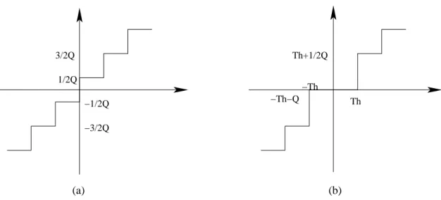
(26) Table 2.1: Weighting Values H0 (i, j), H1 (i, j), and H2 (i, j) H2 (i, j). H1 (i, j). H0 (i, j). 4. 5. 5. 5. 5. 5. 5. 4. 2. 2. 2. 2. 2. 2. 2. 2. 2. 1. 1. 1. 1. 1. 1. 2. 5. 5. 5. 5. 5. 5. 5. 5. 1. 1. 2. 2. 2. 2. 1. 1. 2. 2. 1. 1. 1. 1. 2. 2. 5. 5. 6. 6. 6. 6. 5. 5. 1. 1. 1. 1. 1. 1. 1. 1. 2. 2. 1. 1. 1. 1. 2. 2. 5. 5. 6. 6. 6. 6. 5. 5. 1. 1. 1. 1. 1. 1. 1. 1. 2. 2. 1. 1. 1. 1. 2. 2. 5. 5. 6. 6. 6. 6. 5. 5. 1. 1. 1. 1. 1. 1. 1. 1. 2. 2. 1. 1. 1. 1. 2. 2. 5. 5. 6. 6. 6. 6. 5. 5. 1. 1. 1. 1. 1. 1. 1. 1. 2. 2. 1. 1. 1. 1. 2. 2. 5. 5. 5. 5. 5. 5. 5. 5. 1. 1. 2. 2. 2. 2. 1. 1. 2. 2. 1. 1. 1. 1. 2. 2. 4. 5. 5. 5. 5. 5. 5. 4. 2. 2. 2. 2. 2. 2. 2. 2. 2. 1. 1. 1. 1. 1. 1. 2. resents the residual error remaining after motion-compensated prediction. The texture coder includes padding process (for object-based coding, and applied only if needed), 8 × 8 two-dimensional (2D) discrete cosine transform (DCT), quantization, coefficient prediction, coefficient scan and VLC. We describe the last four elements below.. Quantization MPEG-4 video supports two quantization techniques, one referred to as the H.263 quantization method and the other, the MPEG quantization method. The H.263 quantization method is uniform with dead zone for intra and inter AC coefficients and uniform for intra DC coefficients. The MPEG quantization method is uniform. Figure 2.6 shows the quantizer characteristics in H.263. For inter DC and all AC coefficients, input between −Th and +Th is quantized to zero. All coefficients in an MB go through the same quantizer step size Q, which can be changed in increments of 2 from 2 to 62 as desired. In the MPEG quantizer, each coefficient produced by 2D DCT is quantized with a uniform quantizer. The default quantizer matrix is defined as shown in Table 2.2, which can be changed if desired. Typically, the DC coefficients of 8 × 8 blocks belonging to an intra MB are scaled by 11.

(27) 3/2Q. Th+1/2Q. 1/2Q. −Th −Th−Q. −1/2Q. Th. −3/2Q. (a). (b). Figure 2.6: Quantizers in H.263. (a) For intra DC coefficient only. (b) For inter DC and all AC coefficients. a constant scaling factor of 8. However, in MPEG-4 video, a nonlinear scaler as shown in Table 2.3 is used to provide a higher coding efficiency. The characteristics of nonlinear scaling are different between the luminance and chrominance blocks and further depend on the quantizer used for the block.. Intra Prediction After quantization, the DC coefficients and many AC coefficients of an intra block are coded by intra prediction. Intra prediction is a new operation used in MPEG-4 standards to reduce the spatial redundancy between 8 × 8 blocks. There are two types of prediction, DC prediction and AC prediction. Figure 2.7 shows the prediction of DC coefficients in intra 8×8 blocks. The quantized intra coefficients are predicted with three previous decoded DC coefficients. For example, the DC coefficients of block X is predicted from the DC coefficients of blocks A, B and C. Unlike MPEG-2, the prediction in MPEG-4 is gradient based. In computing the prediction of block X, if the absolute value of a horizontal gradient is less than the absolute value of a vertical gradient, then the QDC of block C is used as the prediction, else QDC value of block A is used. The AC prediction depends on DC prediction, as shown in Fig. 2.8. The AC coeffi12.

(28) Table 2.2: Default Quantization Matrix (Q) [2]. Inter. Intra. 8. 16. 19. 22. 26. 27. 29. 34. 16. 16 16. 16. 16 16. 16 16. 16. 16. 22. 24. 27. 29. 34 37. 16. 16. 16. 16. 16. 16. 16. 16. 19. 22. 26. 27. 29. 34. 34. 38. 16. 16. 16. 16. 16. 16. 16. 16. 22. 22. 26. 27. 29. 34. 37. 40. 16 16. 16 16. 16 16. 16 16. 22. 26. 27. 29. 32. 35. 40 48. 16. 16. 16. 16. 16. 16. 16. 16. 26. 27. 29. 32. 35. 40. 48. 58. 16. 16. 16. 16. 16. 16. 16. 16. 26. 27. 29. 34. 38. 46. 56. 69. 16. 16. 16. 16. 16. 16. 16 16. 27. 29. 35. 38. 46. 56. 69. 83. 16. 16. 16. 16. 16. 16 16. 16. Table 2.3: Nonlinear Scaler for DC Coefficients (from [2]). Component. DC Scaler for Q Range. 1–4. 5–8. 9–24. 25–31. Luminance. 8. 2Q. Q+8. 2Q+16. Chrominance. 8. (Q+13)/2. Q+16. cients in the first row or in the first column are predicted with three previous decoded AC coefficients. The direction of prediction is the same as DC prediction.. Scan and VLC The predicted DC and AC coefficients (as well as the un-predicted AC coefficients) of DCT blocks are scanned by one of three scans: alternate-horizontal, alternate-vertical and zigzag (the normal scan used in H.263 and MPEG-1) to change the 2D image to one dimensional data, as shown in Fig. 2.9. The actual scan used depends on the coefficient prediction method used. For instance, if the DC prediction refers to the horizontally adjacent block, alternate-vertical scan is selected for the current block. If the DC prediction refer to the vertically adjacent block, alternate-horizontal scan is used for the current block. For all other blocks, the 8 × 8 DCT blocks are zigzag scanned. 13.

(29) 0 0 B 000 C 00 D 0or0 0 0 0 0 0 0 0 0 0or0 0 0 0 0 0 0 0 0 0 0 0 0000000000000000000000000000 00 00 00 00 00X00 00 00 00 00 00 00 00 00 00Y00 00 00 00 00 00 00 Macroblock A 0000000000000000000000 00 00 00 00 00 00 00 00 00 00 00 00 00 00 00 00 00 00 00 00 00 00 0000000000000000000000 Figure 2.7: Prediction of DC coefficients of blocks in an intra MB (from [3]).. 00000000000000000 00000000000000000 00000000000000000 00000000000000000 C. B. 00 00 00 000 00 00 00 00 00 00. D. 000 000 000 000 000 000 000 000 000 000 000 000 000 000 000 000 000 000 000 000or000 000 000 000 000 000 000 000 000 000 000 000 000 000 000 000 000 000 000 000 000 000 000 000 000 000 000 000 000 000 000 000 000X000 000 000 000 000 000 000 000 000 000 000 000 000 000 000 000 000 000 000 000 Y000 000 000 000 000 000 000 000 000 000 000 000 000 000 000 000 000 000 000 000 000 000 000 000 000 000 000 000 000 000 000 000 000 000 000 000 000 000 000 000 000 000 000 000 000 000 000 000 000 000 000 000 000 000 000 000 Macroblock 000 000 000 000 000 000 000 000 000 000 000 000 000 000 000 000 000 000 000 000 000 000 000 000 000 000 000 000 000 000 000 000 000 000 000 000 000 000 000 000 000 000 000 0000000000000000000000000000000000000000000 00 00 00 00 00 00 00 00 00 00 00 00 00 00 00 00 00 00 00 00 00 00 00 00 00 00 00 00 00 00 00 00 00 00 00 00 00 00 00 00 00 00 00. or. A. Figure 2.8: Prediction of AC coefficients of blocks in an intra MB (from [3]). The coefficients after scan usually become data with many zeros at the end. This kind of a data stream is good for run-length coding. In MPEG-4, differential DC coefficients in intra blocks are encoded in VLC. But the AC coefficients are encoded by the variable length codes for EVENTs. An EVENT is a combination of a last non-zero coefficient indication, the number of successive zeros preceding the coded coefficient (RUN), and the non-zero value of the coded coefficient (LEVEL). Some statistically rare events have no VLC words to represent them. For them an escape coding method is used.. 14.

(30) Figure 2.9: Scans for 8 × 8 blocks (from [2]).. 2.3.2 Other Video Coding Tools [3] In addition to texture video coding, there are some special tools defined in MPEG-4. We briefly introduce robust video coding and scalable coding here.. 2.3.3 Robust Video Coding Error resilience is a particular concern over wireless networks. In the error resilient mode, the MPEG-4 video offers a number of tools as follows: 1. Object priorities: The object based organization of MPEG-4 video facilitates prioritizing of the semantic objects based on their relevance. Further, the VOP types are a form of inherent prioritization since B-VOPs do not contribute to error propagation and thus can be transmitted at a lower priority or discarded in case of severe errors. 2. Resynchronization: The encoder can enhance error resilience by placing resynchronization (resync) markers in the bitstreams with approximately constant spacing, such as beginning of each MB. 3. Data partitioning: Data partitioning provides a mechanism to increase error resilience by separating the normal motion and texture data of all MBs in a video packet and send all of the motion data followed by a motion marker, followed by all of the texture data.. 15.

(31) 4. Reversible VLCs: The reversible VLCs offer a mechanism for a decoder to recover additional texture data in the presence of errors since the special design of reversible VLCs enables decoding of codewords in both the forward (normal) and the reverse direction. 5. Intra update and scalable coding: Intra update is a simple method to reduce error propagation. However, more intra updates means less coding efficiency. Another method is scalable coding, which can alleviate error propagation without more intra coding.. 2.3.4 Scalable Coding The scalability tools in MPEG-4 video are designed to support applications beyond that supported by single layer video, such as internet video, wireless video, multi-quality video services, video database browsing, etc. In scalable video coding, it is assumed that given a coded bitstream, decoders of various complexities can decode and display appropriate reproductions of coded video. MPEG-4 video provides several different forms of scalability. The basic scalability tools offered are temporal scalability and spatial scalability. A Fine Granularity Scalability (FGS) is also defined which supports continuous scalability of bit rate and video quality.. 2.4. Profiles and Levels [2]. Although there are many tools in the MPEG-4 standard, not every MPEG-4 decoder will have to implement all of them. Similar to MPEG-2, profiles and levels are defined as subsets of the entire bitstreams syntax of all the tools. The purpose of defining conformance points in the form of profiles and levels is to facilitate interchange of bitstreams among different applications. There are eight profiles defined in MPEG-4: simple, core, main, simple scalable, animated & mesh, basic animated texture, still scalable texture and simple face. The details are given in Table 2.4.. 16.

(32) Compared with the previous standards, the simple profile of MPEG-4 is similar to the coding method in H.263. The difference is that the simple profile has error resilience but does not have B-frame coding. The simple scalable profile is simple profile with rectangular scalability. The core profile is the profile with all tools of the simple profile, temporal scalability, B-VOP coding and binary shape coding. The main profile is the profile with all tools in core profile, gray shape coding, interlace and sprite coding. The other profiles are for particular purposes, such as 2D dynamic mesh coding and facial animation coding. For frame-based coding and decoding, what concerns us is the main profile, excluding the shape coding, interlace, and sprite coding tools.. 17.

(33) Table 2.4: Profiles and Tools (from [2]) Simple. Core. Main. Tools. Simple. Animated. Basic. Still. Simple. Scalable. 2D Mesh. Animated. Scalable. Face. Texture. Texture. V. V. V. V. V. Basic. 1. I VOP. 2. P VOP. V. V. V. V. V. V. V. V. V. V. V. 3. AC/DC Prediction. 4. 4MV Unrestricted MV. Error resilience. 1. Slice Resynchronization. 2. Data Partitioning. 3. Reversible VLC. V. V. V. B-VOP. V. V. Method 1/Method 2. V. V. V. V. V. V. V. V. V. Short Header. V. V. quantization. P-VOP based. temporal scalability. 1. Rectangular. 2. Arbitrary Shape. Binary Shape. Gray Shape. V. Interlace. V. Sprite. V. V. Temporal scalability. (rectangular). V. Spatial scalability. (rectangular). Scalable still. texture. 2D dynamic mesh. with uniform topology. V. 2D dynamic mesh. with Delaunay topology. V. Facial animation. parameters. 18.

(34) Chapter 3 Overview of The PACDSP The contents of this chapter have been taken to a large extent from [1].. 3.1. Introduction. Programmable embedded solutions are attractive for their lower development effort, upgradeability to support new applications and easier maintenance. These factors reduce time-to-market and extend time-in-market, and thus make the best profit-sense. Today’s media processing demands extremely high computations with real-time constraints in audio, image or video applications. Instruction parallelism has been exploited to speed up the high-performance microprocessors, and VLIW machines have low-cost compiler scheduling with deterministic execution time and have thus become the trend of high performance DSP processors. Conventional VLIW processors are notorious for their poor code density, because the unused instruction slots must be filled by NOPs. Thus, the code density gets worse when the parallelism is limited. Variable-length VLIW instruction packet eliminates NOPs by dispatching instructions at run-time, compared to the conventional position-coded VLIW processors where each functional unit (FU) has a corresponding bit-field in the instruction packet. Indirect VLIW has an internal instruction buffer for the VLIW instruction packets. With this instruction buffer and the pre-fetch scheme, the VLIW processor can reduce instruction memory bandwidth requirement and power consumption of instruction 19.

(35) fetches. The complexity of the register file (RF) grows exponentially as more and more FUs are integrated on a chip, which operate concurrently to achieve the performance requirements. The RF is frequently partitioned for execution clusters with explicit interconnection networks among the clusters to significantly reduce the complexity at the cost of small performance penalty. For high performance, the PACDSP is a VLIW processor with single instruction multiple data (SIMD) instruction set architecture (ISA). The software supported schedule reduces the complexity of hardware design and the power consumption. Variable length instruction and instruction packet solve the poor code density problem of the conventional VLIW architecture. Another feature of the PACDSP, cluster architecture, reduces not only ports and entries of the register files but also the power consumption of read/write operations. More details about the features of PACDSP are discussed in the following sections.. 3.1.1 Architecture Features Key features of the PACDSP include the following items: • Scalable VLIW datapath for easy extension of the performance. • Variable instruction word/packet length to avoid the drawback of poor code density in the conventional VLIW architecture. • Heterogeneous register files for more straightforward operations, less ports and smaller entries in each RF to improve the performance and reduce power and area. • Constant register file in each cluster (32×32 bits) for storage of some fixed data in the applications to reduce the frequency of data movement which may cost significant of power consumption. • Inter-cluster communication (ICC) by memory controller for reusing hardware resource and reducing the port number of ping-pong RF in order to reduce power and area and to increase the scalability.. 20.

(36) • Optimized interrupt design with fast interrupt response time (3 clock cycles) with hardware supporting context switch to reduce the processing time of interrupt service routine (ISR). • Hierarchical encoding scheme reducing the dependency between instructions and packets to reduce area and latency of the dispatch unit. • Dynamic power management for power saving. • Customized instruction set and functional unit interface for the accelerators that are used to enhance certain DSP operations.. 3.2. Architecture Overview. There are three components in the PACDSP kernel: program sequence control unit, scalar unit and VLIW datapath. The accelerators that execute in different threads and synchronize the execution results through the scalar unit can enhance the computation power of the VLIW datapath. Figure 3.1 shows the architecture of the PACDSP. The program sequence control unit dispatches instructions to the scalar unit and the VLIW datapath. It also executes control flow instructions and handles the interrupt and exception events. The scalar unit executes the scalar instructions whose characteristics are low parallelism and high data dependency. It also controls the power control interface and the customized functional unit interface. The VLIW datapath composed of two clusters takes charge of complex data operations in the program. Each cluster contains a load/store unit (L/S) and an arithmetic unit (AU). Both units can execute instructions concurrently. Another feature of the PACDSP, the ping-pong register file, facilitates data transfers between these two units. With this feature, the typically high power consumption of the DSP kernel can be reduced. The maximum parallelism of the VLIW datapath in instruction and operation levels is 4 and 12, respectively.. 21.

(37) Figure 3.1: Architecture of the PACDSP [1].. 3.3. Program Sequence Control Unit. The program sequence control unit is a main component in the DSP kernel. It dispatches instructions to the scalar unit and the VLIW datapath. It also executes the execution flow control instructions and handles the interrupt and exception events.. 3.3.1 Branch Instruction Branch instructions can be grouped into two categories, conditional branches and unconditional branches. There are three addressing modes defined in the PACDSP for generating the branch target address: • PC-relative Add the 16-bit signed immediate offset to the address in the PC register, and take the result as the branch target address, i.e.,. 22.

(38) TA = PC + OFFSET where TA is the target address, PC is the address in PC register, and OFFSET is the 16-bit signed immediate value. • Register Take the value in the register as the target address, i.e., TA = Rs where TA is the target address and Rs is the source register of address. • Register-relative Add the 16-bit signed immediate offset to the address saved in the register and take the result as the branch target address, i.e., TA = Rs + OFFSET where TA is the target address, Rs is the source register saving the address, OFFSET is the 16-bit signed immediate value. The branch instructions defined in the PACDSP support saving of the return address into the assigned register. The programmer should take care of the return addresses of nested loops. There are three branch delay slots in the PACDSP, and the independent instructions can be put in these delay slots.. 3.3.2 Loop The programmer can use the LBCB instruction to effect program loops. Loop Boundary Register (RBC0 – RBC3), which are all 32-bit registers, can be used to record the loop counts. However, the maximum loop count is 65536 for each level. Since there are four Loop Boundary Registers, up to four levels of nested loop can be supported with the use of the LBCB instruction.. 23.

(39) There is a constraint in using LBCB to control a nested loop. The outer loop should fully contain the inner loop. No exception will be generated if the constraints are violated, but the program behavior may be different from expectation. However, conditional branches can be used inside the nested loop to implement some special branch behaviors in higher level languages, for example, “break” and “continue” in C.. 3.3.3 Customized Function Unit (CFU) The PACDSP provides Customized Function Unit Interface for extension purpose. The user can attach co-processors or customized function units to PACDSP and handle them through the scalar instructions. If some error happens in a customized function unit, it can inform the PACDSP and the PACDSP can process it based on the particular configuration. If the work given is finished successfully, the PACDSP can use its results and continue to work. It is recommended to use this interface to communicate with any added coprocessor; otherwise, the user may have to pay significantly more effort to handle it.. 3.3.4 Exception Handling Unpredictable exceptions may occur during program execution. The exceptions need to be handled correctly for correct execution results. Exceptions may be caused by hardware (e.g., overflow), software, internal (e.g., undefined instruction), or external (e.g., coprocessor exception). When an exception happens, the DSP kernel will be frozen or listen to the main processing unit (MPU) deliverance. It is still aware of debug requests and will check the corresponding signal to see what kind of exceptions have happened.. 3.3.5 Interrupt Handling Two types of interrupt are supported by the PACDSP. One is fast interrupt request (FIQ), which has the higher priority, and the second is interrupt request (IRQ). The difference between them is that the FIQ uses hardware to reduce the time in saving the context and. 24.

(40) the hardware resources used for the FIQ interrupt service routine (ISR) consist only of the scalar unit and program sequence control unit. Contrarily, the IRQ can use all the hardware resources in PACDSP to deal with the IRQ request, but the ISR of IRQ needs to save the context by itself. In the PACDSP, the minimum latency from interrupt request to the first ISR instruction to be executed is 3 cycles for both types of interrupt, and it may be postponed when the ISR experiences cache miss.. 3.4. VLIW Datapath. 3.4.1 Ping-Pong Register File A centralized register file (RF) provides storage for and interconnects to each functional unit (FU), and each FU can read from or write to any register location. But in practical designs, the communication between FU is usually restricted by partitioning the RF to reduce the complexity significantly with some performance penalty. In other words, each FU can only read and write a limited subset of registers. In the ping-pong hierarchical RF, which is shown in Fig. 3.2, the RF is partitioned into private and ping-pong subblocks. Each FU (L/S or AU) can simultaneously access two sub-blocks, one of which is private (i.e., dedicated to the FU) and the other is dynamically mapped for inter-FU communications within one cluster. Therefore, each sub-block only requires the access ports for a single FU. The shared sub-blocks are organized in a ping-pong fashion to reduce the control overheads, where the dynamic mapping is exposed to the VLIW ISA with two switching bits and is directly specified by the programmers for each instruction packet.. 3.4.2 Data/Address/Accumulator Registers As shown in Fig. 3.3, the address registers (A0–A7) are all 32-bit and they are dedicated to the load/store unit (L/S) for memory accesses. In addition, A1, A3, A5, and A7 are also treated as the base registers which contain the base addresses in modulo addressing mode. 25.

(41) Private Registers. A0 − A15 (32−bit). L/S. D0 − D7 (32−bit) Ping−Pong Register. 2−bit configuration. D8 − D15 (32−bit) AU AC0 − AC7 (40−bit). Private Registers. Figure 3.2: Ping-pong register file in one cluster [1]. E0–E3 (A8, A10, A12, and A14) and D0–D3 (A9, A11, A13, and A15) are individually treated as end registers and displacement registers which contain end addresses and displacements in modulo addressing mode. Nevertheless, in linear addressing mode, they can be treated as the address register like A0–A7. The accumulator registers (AC0–AC7) are 40-bit (8-bit as guard bits) and are dedicated to the arithmetic unit(AU) for data manipulations. The data registers(D0–D7 and D8–D15) are organized in the form of ping0pong with 1-bit control and the word-length of these registers are 32-bit.. 3.4.3 Status and Control Registers The status register and control register which are read and set by instructions can be used to monitor the DSP kernel status and handle the operation mode of DSP kernel.. 26.

(42) D0.H. D0.L. D8.H. D8.L. AC0.G. AC0.H AC0.L. A0. A8/E0. D1.H. D1.L. D9.H. D9.L. AC1.G. AC1.H AC1.L. A2. A10/E1. D2.H. D2.L. D10.H D10.L. AC2.G. AC2.H AC2.L. A4. A12/E2. D3.H. D3.L. D11.H D11.L. AC3.G. AC3.H AC3.L. A6. A14/E3. D4.H. D4.L. D12.H D12.L. AC4.G. AC4.H AC4.L. A1/B0. A9/D0. D5.H. D5.L. D13.H D13.L. AC5.G. AC5.H AC5.L. A3/B1. A11/D1. D6.H. D6.L. D14.H D14.L. AC6.G. AC6.H AC6.L. A5/B2. A13/D2. D7.H. D7.L. D15.H D15.L. AC7.G. AC7.H AC7.L. A7/B3. A15/D3. Data Register 32−bit (L/S). Data Register 32−bit (AU). Accumulater Register 40−bit (AU). Address Register 32−bit (L/S). End/Displacement Register 32−bit (L/S). Figure 3.3: The available registers in one cluster [1]. Program Status Register The 16-bit program status register records the operation status in each cluster and the scalar unit. It includes Overflow, Negative, and Carry bits, and instructions can only read the status register, not set it. Addressing Mode Control Register (AMCR) The PACDSP provides three types of addressing modes: • Linear addressing mode, • Bit-reverse addressing mode, • Modulo addressing mode. As shown in Fig. 3.4, the addressing mode control register (AMCR) is a 32-bit read/write register. This register is used to control the addressing mode of relative address registers. The addressing modes are related to where the operands are to be found and how the address calculations are to be made.. 27.

(43) AMCR Addressing Mode Control Register 32 − bit Reserved [31:16]. A7 [15:14]. AM[1]. AM[0]. Addressing Mode. 0. 0. Linear. 0. 1. 1. 0. Modulo. 1. 1. Reserved. A6 [13:12]. A5 [11:10]. A4 [9:8]. A3 [7:6]. A2 [5:4]. A1 [3:2]. A0 [1:0]. Bit−Reverse. Figure 3.4: Illustration of the addressing mode control register (AMCR) [1].. 3.4.4 Addressing Modes The addressing modes are related to where the operands are to be found and how the address calculations are to be made. Linear Addressing Mode There are three kinds of linear addressing mode, which are register direct mode, address register indirect mode, and immediate data mode. The register direct addressing mode specifies that the operand is in one or more of the arithmetic unit (AU) registers, load/store unit (L/S) registers, control registers and program counter (PC) registers. This addressing mode is also used to specify a control register operand and a PC register operand for special instructions. The address register indirect mode specifies that the address register is used to point to a memory location. The term indirect is used because the register contents are not the operand itself, but the operand address. This addressing mode specifies that an operand is in a memory location and specifies the effective address of that operand. There are still two sub-modes in the address register indirect mode: • Pre-increment, +(Rs) offset The operand address is the sum of the contents of the address register and the offset. The data stored at the address of the sum of register value and offset will be loaded. 28.

(44) • Post-increment, (Rs)+ offset The operand is in the address register Rs. After the operand address is used, it is incremented by the offset and stored in the same address register. Incrementing the operand address by the offset places the next available address in the register. That is, the data stored at the location of the address register will be loaded first, and then the address is updated with the offset. The immediate data mode does not use an address register. The instructions use an immediate value that is included in the instruction for the data value or address value. Bit-Reverse Addressing Mode Bit-reverse addressing mode is also called reverse-carry addressing mode. It is useful for 2k -point FFT addressing. This mode is selected by setting the corresponding bits in AMCR, and address modification is performed in the hardware by propagating the carry from each pair of added bits in the reverse direction (from the MSB end toward the LSB end). It can also use the pre- or post-increment addressing mode. This address modification is useful for addressing the twidle factors in 2k point-FFT addressing as well as to unscramble 2k -point FFT data. Modulo Addressing Mode Modulo address modification is useful for creating circular buffers for FIFO queues, delay lines, and sample buffers. The definition of modulo addressing, using a base register (Bn) and a modulo register (M i), enables the programmer to locate the modulo buffer at any address. The address pointer, An, is not required to start at the lower address boundary, nor to end on the upper address boundary. It can initially point to anywhere (aligned to its access width) within the defined modulo address range, Bn ≤ An < Bn + M i. Modulo addressing can be selected by configuring corresponding bits in AMCR, and write the desired modulo to modulo registers. The range of modulo registers, M i, is from 1 to 232 − 1.. 29.

(45) Each base address register (Bn) is associated with an address register (B0 with A0, and so on). Offset and modifier registers are also associated with the corresponding address registers in the same way.. 3.4.5 VLIW Datapath The VLIW datapath of PACDSP is constructed in two clusters, and each contains an arithmetic unit (AU) and a load/store unit (L/S) as shown in Fig. 3.2. Therefore, it can execute four instructions simultaneously, and is thus called a four-way VLIW datapath. Arithmetic Unit (AU) The arithmetic unit (AU) comprises four 40-bit adders which can be reconfigured to two 16-bit adders or four 8-bit adders, two 16-bit multipliers, one shifter and one logical ALU. All data processing instructions in AU begin at the same stage, but not finish at the same time. There are three types of precision in DSP — full, integer, and fractional. Figure 3.5 shows how it works. • Full precision: Rd = Rs1.L × Rs2.L. • Integer: Rd.L = (Rs1.L × Rs2.L)[15:0]. • Fractional: Rd.L = Rs1.L × Rs2.L)[30:15]. Load/Store Unit (L/S) The load/store unit (L/S) comprises one address generation unit (AGU), one logical ALU, and one shifter. Similar to AU, all instructions in L/S begin at the same stage, but not finish at the same time. The L/S unit supports powerful double load/store instructions, which can load or store two operands in one instruction. Figure 3.6 shows how double and vector load/store work.. 30.

(46) Rs1.L. Rs2.L. Rd.H. Rd.L. Full Precision Rs1.L. Rs2.L. 111111111111111111 000000000000000000 111111111111111111 000000000000000000 111111111111111111 000000000000000000 111111111111111111 000000000000000000 111111111111111111 000000000000000000. Rd.L. Integer. Rs1.L. 11 00 11 00 11 00 11 00 11 00. Rs2.L. 111111111111111111 000000000000000000 111111111111111111 000000000000000000 111111111111111111 000000000000000000 111111111111111111 000000000000000000 111111111111111111 000000000000000000. Rd.L. Fractional. Figure 3.5: Illustration of multiplication instructions with different precisions [1].. 3.4.6 Data Exchange As shown in Fig. 3.7, the PACDSP provides a data exchange mechanism between any two of the scalar unit and the two clusters. Figure 3.8 shows that it can also provide data broadcast to facilitate one of them to broadcast its data to the others even though the number of clusters may be extended someday. This job is accomplished by using the ports of the memory interface unit (MIU) because MIU has connections with all register files of the scalar unit and the two clusters. Data Exchange Between Clusters The PACDSP provides a special instruction (DEX) to accomplish data exchange between clusters. For example: Cluster1 instruction: DEX D1, D0 Cluster2 instruction: DEX D1, D2 31.

(47) Load/Store. Load/Store Unit. Unit. D0. D1. D0.H. D0.L. D2. D3. D1.H. D1.L. D4. D5. D2.H. D2.L. D6. D7. D3.H. D3.L. Double Load//Store. Vector Load/Store. Figure 3.6: Different load/store instructions [1]. At compile time, this instruction pair will cause direct exchange of the contents of D0 and D2 through MIU and each cluster will store them in D1, as shown in Fig. 3.7. Data Broadcast Like data exchange between clusters, PACDSP also provides a special instruction pair (BDT and BDR) for data broadcast from one cluster to the others. For example: Cluster1 instruction: BDT D0 Cluster2 instruction: BDR D3 Scalar instruction: BDR R0 At compile time, this set of instructions will broadcast data from cluster1 to cluster2 and the scalar unit as shown in Fig. 3.8. On the other hand, if we just want to transmit data from one cluster to another (including the scalar unit), it can be considered a special case of data broadcast. For example: Cluster1 instruction: ADD D0, D1, D2 Cluster2 instruction: BDR D7 Scalar instruction: BDT R0 In this example, the content of R0 is transmitted to D7 in cluster2. At the same time, 32.

(48) MIU. Scalar Unit. Load/Store Unit. Load/Store Unit. Arithmetic Unit. Arithmetic Unit. Cluster1. Cluster2. Figure 3.7: Data Exchange between Two Clusters [1]. MIU. Scalar Unit. Load/Store Unit. Load/Store Unit. Arithmetic Unit. Arithmetic Unit. Cluster1. Cluster2. Figure 3.8: Data broadcast among clusters [1]. cluster1 can do other operations without affecting by this transmission.. 3.4.7 Constant Register File In many DSP algorithms, such as FIR, IIR, etc., there are many coefficient operations which use fixed data. In order to avoid high frequency of data movement in the register file, the PACDSP provides a small size memory, called Constant Register File to maintain the fixed data. We can also use it to store look up tables which contain fixed data for specific applications. It can reduce the frequency of data movement and thereby reduce power consumption in such operations. Data contained in the Constant Register File can be used to do operations including 33.

(49) comparison, multiplication, multiplication and accumulation, etc. They are used as the second source operand in the instructions. The specifications of Constant Register File (in one cluster) are as follows: • 32 × 32 bits. • Two read ports and one write port. As shown in Fig. 3.9, the Constant Register File is initialized through the write port by MIU at the beginning of the program. Not only the L/S but also the AU has a read port for taking its value as one source operand. There are some rules when using the Constant Register File: • It can only be modified by particular instructions in L/S. • Read and write operations may not occur at the same time in L/S.. 3.5. Scalar Unit. 3.5.1 Overview The Scalar Unit can perform three types of function, which are basic arithmetic operations, word and halfword-based load/store operations, and read/write operations performed on the contro/status registers. Under some running modes, the DSP core may execute a program without activating the VLIW clusters. In this case, the scalar unit acts like a simple machine, handling some easy tasks. Mostly, the scalar unit is in charge of the control-based work while the VLIW clusters are dealing with data processing. Data can be exchanged between the scalar unit and the VLIW clusters.. 3.5.2 Control Registers In the PACDSP kernel, there are 15 control registers. Table 3.1 shows the names and the widths of all the control registers in the PACDSP kernel. 34.

(50) Memory Interface Unit (MIU) Private RF. Load/Store Unit Customized FU. Coefficient Public Ping−Pong RF. Memory Arithmetic Unit Customized FU. Private RF. Figure 3.9: The Constant Register File of one cluster [1]. Several control registers are memory mapped and can be accessed by others outside the PACDSP kernel. Table 3.2 lists the memory mapped control registers and the mapping memory addresses. The control registers can be read or write by the scalar instructions. When writing the control registers, we can assign a 16-bit immediate value to the destination, or set a general purpose scalar register as the source operand.. 3.5.3 General Purpose Scalar Register File In the scalar unit of the PACDSP kernel, there are sixteen 32-bit general purpose registers named R0 to R15.. 35.

(51) Table 3.1: Details of Control Register Files [1] Type. Control. No. Name. Note. Size(bits). CR0. PREDN. 16. Prediction information. CR1. EN INT. 1. Interrupt enable flag. CR2. MSK EX. 16. Mask inside exception. CR3. SWI EX. 16. Software exception. CR4. CF0. 32. Custom function register 0. CR5. CF1. 32. Custom function register 1. CR6. CF2. 32. Custom function register 2. CR7. CF3. 32. Custom function register 3. CR8. SD MIXIFN0. 32. Mix information 0’s shadow register. CR9. SD Rbc1. 32. Loopboundary counter’s shadow. register1. CR10. SD Rbc2. Loopboundary counter’s shadow. 32. register2. Interrupt. CR11. SD BCTG. 32. Branch target shadow register. CR12. SD CPC. 32. CPC’s shadow register. (ISR return address). CR13. SD PREDN. 16. Prediction’s shadow register. CR14. SD R0. 32. R0’s shadow register. Reserved. CR15. 3.6. Conditional Execution Control. Unlike general purpose processors, the major mission of a DSP is to provide more computing power for calculations. To reduce control overhead, the PACDSP supports conditional execution of instructions. Programmers can set predicates by Compare-and-Set instructions and then the instructions afterward can refer to the predicates to decide whether to execute or not. When the program calls a function, we can save the predicates and restore them after returning from the function call. The Compare-and-Set instructions, such as SLT, SGT, etc., compare source operands 36.

(52) Table 3.2: Memory-Mapped Control Registers [1] R/W. Note. Offset. 32. Indicate inside exception cause. 0x50020. R. Busy. 1. DSP is busy. 0x5000C. R. 02. Start. 1. Start signal. 0x50008. R/W. 03. Start PC. 32. Starting address. 0x50000. R/W. 04. MODE. 4. DSP running mode. 0x50040. R. 05. VERSN. 4. DSP version. 0x50044. R. No. Name. 00. Exception Cause. 01. Size. and save the results to the predicate registers, and the comparison results can be saved to the general purpose registers at the same time. The PACDSP provides 16 predicate bits (P0–P15), and a Compare-and-Set instruction updates 2 predicate bits at the same time. However, P0 is always set to 1, and each predicate bit can be set by only one instruction at the same time.. 3.7. ISA and Pipeline Stages. As said, the PACDSP architecture consists of the program sequence control unit, the scalar unit, and the VLIW datapath. Each of the three has corresponding function units. Therefore, the instruction set of PACDSP is classified according to the functional unit in which the instruction is executed. Figure 3.10 depicts the instruction set architecture (ISA) of the PACDSP. Figure 3.11 shows the pipeline stages of the PACDSP. The program sequence control can be divided into three stages, which are IF, IDP, and ID. The scalar unit operation and the VLIW datapath are both divided into five stages, which are RO, EX1, EX2, EX3, and WB. The job of each pipeline stage is as described in Table 3.3.. 37.

(53) PACDSP ISA. Program Sequence. Scalar. Program Control. CR. Load/ Store. VLIW. AU. Load/ Store. AU. Figure 3.10: PACDSP instruction set architecture [1]. Program Sequence Control Unit IF. IDP. VLIW Datapath ID. RO. EX1. EX2. EX3. WB. Scalar Unit. Figure 3.11: Pipeline stages of the PACDSP [1].. 3.8. DSP Running Modes. The PACDSP can work under various running modes. Each mode has different hardware utilization. There are 7 different running modes. The corresponding hardware resource and a simple description of each running mode is given in Table 3.4. It is noted that not all running modes can be chosen to be entered by the instructions. We can only change the three sub-modes of the the user mode by the instructions. The transitions between running modes are shown in Fig. 3.12.. 38.

(54) Table 3.3: Pipeline Stages and Their Descriptions Stage. Description. IF. Instruction Fetch. IDP. Instruction Dispatch. ID. Instruction Decode. RO. Read Operand. EX1. Execution One. EX2. Execution Two. EX3. Execution Three. WB. Write Back. 3.9 Instruction Packet The PACDSP can issue up to 5 instructions in one cycle. Instructions issued in the same cycle are packeted into an instruction packet. The five slots of the instruction packet and the types of instruction that can be contained in each slot are listed in Table 3.5. The whole instruction packet is bounded by brackets, and slots within packet are separated by new-line characters. Figure 3.13 shows the syntax of a complete instruction packet. However, an instruction packet is allowed to be written in a single line, and be separated by a pipe character “|”. The simplified syntax is shown in Fig. 3.14. It is noted that a NOP instruction should be placed in the slot where there is no instruction to be executed.. 3.10. Development Tools and Implementation Considerations. 3.10.1 Development Tools We have a C-compiler ported from the well-known Open-Research-Compiler (ORC) on linux systems, and we can give parameters to optimize the performance of compiler. How-. 39.

(55) Table 3.4: Running Modes of the PACDSP [1] Description. Running Modes. Idle Mode. Resources. Idle after reset. Execution control. or trap. and interrupt interface. Process program. High Performance. which needs all resources. All available. Process program. User Mode. Medium Performance. which does not need. All except Cluster 2. all resources. High power saving. Wait Mode. Frozen Mode. Process FIQ ISR. All except Cluster 1. or scalar program. and Cluster 2. Wait for Customized. CFU, interrupt,. Function Unit. debug interface, and. result. exception handling unit. Froze DSP since. Debug and interrupt interface,. exceptions happened. exception handling unit. Debug interface,. Debug Mode. Debugging. register files. ever, we can choose only one optimization level to the current status. In addition, base utilities are ported from the GNU binutils, and there are assembler, linker, and other object handling tools. The debugger is ported from the GNU GDB, and GDB is an abbreviation of GNU project debugger. The debugger can be connected to both the instruction set simulator (ISS) and embedded ICE. These tool chains are developed by Programming Language Laboratory of National Tsing Hua University in Hsinchu, Taiwan, R. O. C.. The ISS is developed by SoC Technology Center (STC) of Industrial Technology Research Institute of Taiwan, R. O. C.. The input file of the simulator is split through a parsing tool, “as2tic”, which parses the assembly code into two parts, data and instruction. We can configure the ISS to decide which kinds of information we want to print out to files. All the registers can be shown in each cycle, but the printable memory range is 8 40.

(56) Figure 3.12: Transitions between DSP running modes [1].. Table 3.5: Instruction Type in Each Instruction Slot Instruction Slot. Instruction Types. 1 (Scalar Unit). Program Sequence Control Instructions. 2 (Cluster1). VLIW Load/Store Instructions. 3 (Cluster1). VLIW Arithmetic Instructions. 4 (Cluster2). VLIW Load/Store Instructions. 5 (Cluster2). VLIW Arithmetic Instructions. 41.