考慮井部分貫穿效應之定水頭試驗

國 立 交 通 大 學

環 境 工 程 研 究 所

碩 士 論 文

考慮井部分貫穿效應之定水頭試驗

在非侷限含水層的解

Laplace-domain solution for transient flow into a partially penetrating

well in unconfined aquifers under the constant-head test

研究生 ： 陳 庚 轅

指導教授 ： 葉 弘 德

考慮井部分貫穿效應之定水頭試驗在非侷限含水層的解

Laplace-domain solution for transient flow into a partially penetrating

well in unconfined aquifers under the constant-head test

研 究 生：陳庚轅 Student: Geng-Yuan Chen

指導教授：葉弘德 Advisor: Hund-Der Yeh

國立交通大學

環境工程研究所

碩士論文

A Thesis

Submitted to Institute of Environmental Engineering College of Engineering

National Chiao Tung University in partial Fulfillment of the Requirements

for the Degree of Master of Science

in Environmental Engineering August 2010

Hsinchu, Taiwan

考慮井部分貫穿效應之定水頭試驗在非侷限含水層的解

研究生：陳庚轅 指導教授：葉弘德

國立交通大學環境工程研究所

摘 要

進行定水頭試驗時，需在抽水井中維持固定的水位高，並同時測量觀測井內洩降隨 時間的變化。本研究考慮在非侷限含水層裡有一部分貫穿井作定水頭試驗，推導水層水 位分佈之半解析解。本研究首先將部分貫穿井濾管部分設為定水頭邊界、盲管部分設為 不透水邊界，接著以自由液面條件來描述非侷限含水層的上邊界，最後利用分離變數法 及拉普拉斯轉換，推導得半解析解。此解可用來產生無因次洩降與時間之關係曲線，探 討部分貫穿井在水層中所造成的垂直流問題，亦可利用試驗數據來推求水層的參數。 關鍵詞：地下水，非侷限含水層，部分貫穿，定水頭試驗

Laplace-domain solution for transient flow into a partially penetrating

well in unconfined aquifers under the constant-head test

Student:Geng-Yuan Chen Advisor:Hund-Der Yeh

Institute of Environmental Engineering

National Chiao Tung University

Abstract

The constant head test is to keep constant water level in the pumping well while the

drawdown into the observed well is measured. This study derives a semi-analytical solution

for drawdown distribution during constant-head test at a partially penetrating well in an

unconfined aquifer. The constant-head condition is used to describe the boundary along the

screen while no-flow condition is employed to describe the boundary along the casing of the

well. In addition, a free surface condition is utilized to delineate the upper boundary of the

unconfined aquifer. The Laplace domain solution is then derived using separation of

variables and Laplace transform. This solution can be used to produce the curves of

dimensionless drawdown versus dimensionless time to investigate the effects of vertical-flow

to identify the aquifer parameters from the data of constant-head test.

誌 謝

首先誠摯的感謝指導教授葉弘德，老師悉心的教導使我得以一窺地下水領域的深 奧，不時的討論並指點我正確的方向，使我在這兩年中獲益匪淺。老師對學問的嚴謹更 是我輩學習的典範。本論文的完成另外亦得感謝口試委員台灣大學劉振宇教授、中國科 技大學陳主惠教授、及中興大學謝平城教授有你們的指正及建議，使得本論文能夠更完 整而嚴謹。 除了老師外，最感謝的就是雅琪與彥如學姊，不厭其煩的指出我研究中的缺失，且 總能在我迷惘時為我解惑。感謝智澤、彥禎、玉德、仲豪、珖儀學長、敏筠、其珊學姐、 國豪、玉霖、昭志學弟們，兩年裏的日子，實驗室裏共同的生活點滴，學術上的討論， 感謝眾位學長姐、同學、學弟妹的共同砥礪，你們的陪伴讓兩年的研究生活變得絢麗多 彩。也感謝璟勝，課業的討論和有著趕作業的革命情感。士賓和博傑學長壘球的啟發， 信元、展帆、金澄、阿嚕、家馨、恰恰……排球隊一起運動和比賽，當然還有摯友勝然 和信佑從大學到研究所就一起鼓勵與支持，恭喜我們順利走過這兩年。女朋友怡蓁在背 後的默默支持更是我前進的動力，沒有怡蓁的體諒、包容，相信這兩年的生活將是很不 一樣的光景。 最後，將本論文獻給我最親愛的雙親，冠億，鶴升你們是我最親愛的家人，給我有 形與無形的支柱，謹將這份成果與榮耀與你們分享。

Table of Contents

中文摘要...I

Abstract ... II

誌謝...IV

Table of Contents ... V

LIST OF FIGURES ... VII

NOTATION ... VIII

CHAPTER 1 INTRODUCTION... 1

1.1 Background ... 1

1.2 Literature Review ... 2

1.3 Objectives ... 6

CHAPTER 2 MATHEMATICAL DERIVATIONS... 7

2.1 Mathematical Model of Constant-Head pumping Test ... 7

2.1.1 Governing Equations... 7

2.1.2 Initial and boundary conditions ... 8

2.2 Laplace-domain solution... 10

2.3 Fully penetrating wells in unconfined and confined aquifers ... 12

CHAPTER 3 NUMERICAL EVALUATION ... 13

CHAPTER 4 RESULTS AND DISCUSSION... 16

4.1 Effective distance for the observation well with different specific time ... 16

4.2 Influence of specific yield ... 16

4.3 Effect of screen length ... 17

4.4 Effective distance for the observation well... 17

4.5 Effect of anisotropy ... 18

4.6 Influence of the well radius... 19

4.7 Effect of partially penetration ... 19

CHAPTER 5 CONCLUSIONS ... 20

APPENDIX A... 21

APPENDIX B... 29

APPENDIX C... 33

LIST OF FIGURES

Fig 1. Schematic representation of an unconfined aquifer with a partially penetrating well...41

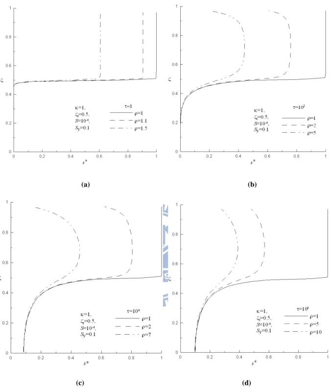
Fig 2. The dimensionless drawdown distributions at τ = (a) 1 , (b) 102 , (c) 104 , and (d) 106 .

...42

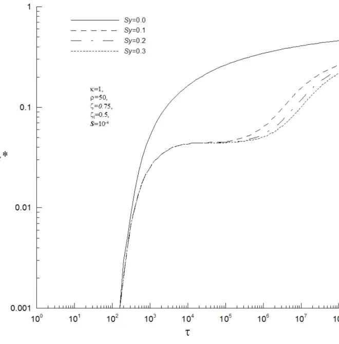
Fig 3. The effect of specific yield on the dimensionless drawdown during CHT. ...43

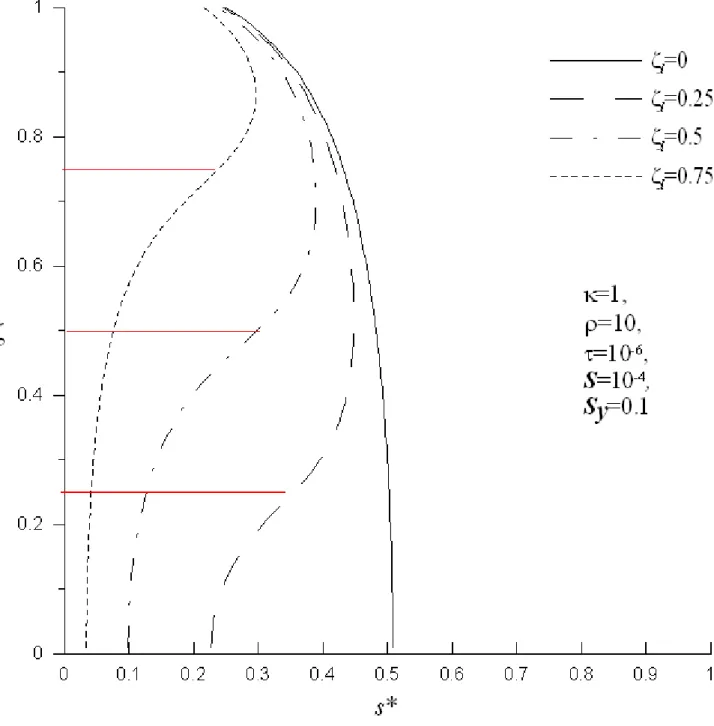
Fig 4. The dimensionless drawdown distributions at the well screen extended from ζ = to ζl

β

ζ = in region 2. ...44

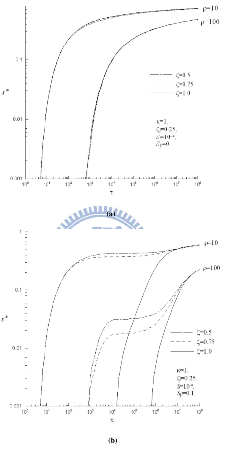
Fig 5. Relationship for dimensionless drawdown versus dimensionless time with ζ =50, 75,

and 100 at ρ =10 or 100 for S = (a) 0 and (b) 0.1... 45 y

Fig 6. Spatial flow pattern in an unconfined aquifer with a partially penetrating well for κ =1,

100 = β , 25ζl = , 4 10− =

S at τ = 104 when S = (a) 0 and (b) 0.1. ... 46 y

Fig 7. The effect of conductivity ratio (κ) of region 2 on the dimensionless drawdown during

CHT. ...47

Fig 8. Drawdown distribution for a well with three different well radii (r = 1, 0.1 and 0.01 m) w

with _{σ =10}3_{, ζ =0.75, 5=0.}

l

ζ and κ =1. ...48

Fig 9. Effect of α on drawdown in a 100 m thick aquifer when _{σ =10}3_{, 1κ = at ζ =0}

NOTATION

′ m A₁ A1m(p)I0( p+ω1m) ′ n A₂ A2n(p)K0( p+ω2n)

b Initial saturated thickness

0 h Initial head h Hydraulic head ) ( 0 ⋅

I modified Bessel functions of the first kinds of order zero

) (

1 ⋅

I modified Bessel functions of the first kinds of order one

m

i₀ I₀( p+ω_1m)/( p+ω_1m ⋅I₁( p+ω_1m))

) (

0 ⋅

K modified Bessel functions of the second kinds of order zero

) (

1 ⋅

K modified Bessel functions of the second kinds of order one

Kr Radial hydraulic conductivity

Kz Vertical hydraulic conductivity

n

k₀ ( p+ω_2n ⋅K₁( p+ω_2n))/K₀( p+ω_2n)

r Radial distance from the centerline of the well

rw Well radius

* 1

s s /1 sw, dimensionless drawdown in region 1

* 2

s s /2 sw, dimensionless drawdown in region 2 ) , , ( ~* 1 P

s ρ ζ dimensionless drawdown in Laplace domain for region 1

(

P

)

s , ,

~*

2 ρ ζ dimensionless drawdown in Laplace domain for region 2

Ss Specific storage

w

s Constant drawdown in the well

Sy Specific yield

t Time from the start of test

z Vertical distance from the bottom of the aquifer

zl Lower z coordinate of well screen

α _{α α ρ}2 w = w α 2 w w κρ α = β b /rw ζ z /b

l ζ zl/ b η _{saturated thickness} ρ ρ=r /r_w w ρ ρw =rw/b σ σ =Sy/Ssb τ Krt/Ssrw2, dimensionless time m 1 ω separation constant n 1 ω separation constant 1 Ω ω1m/αw 2 Ω ω2n/αw

CHAPTER 1 INTRODUCTION

1.1 Background

Groundwater is water stored in aquifers. A unit of rock or an unconsolidated deposit is

called an aquifer when it can yield a usable quantity of water. There are two common types

of aquifers: confined and unconfined. Confined aquifer includes upper and lower confining

beds which are of low permeability. Unconfined aquifers are sometimes also called water

table aquifers, because their upper boundary is a water table.

There are two main hydraulic parameters play a crucial role for the aquifer system in

response to the test: transmissvity and storativity. Transmissivity describes the ease with

which water can move though an aquifer and is a product of hydraulic conductivity and

aquifer thickness. The behavior of hydraulic conductivity is similar to transmissvity.

Hydraulic conductivity has the same unit as velocity. Storativity is defined as the

dimensionless volume of water that an aquifer releases.

Two types of tests, named constant-head test (CHT) and constant-flux test (CFT), are

usually performed to characterize an aquifer for estimating the hydraulic parameters. The

CHT is usually employed for low-transmissivity aquifers, i.e., for aquifers with clay and/or

silt formation. The drawdown/buildup should be kept at a constant value during the test

which are mainly composed of sand and/or gravel materials. The well discharge rate should

be kept at a constant value during the pumping period.

1.2 Literature Review

For aquifers with low-transmissivity, CHT is more suitable to apply than CFT. The

wellbore storage at the pumping well has large effect on the early time drawdown behavior at

pumping and observation wells in CFT (Renard, 2005). If a CHT is established in a short

period of time, the effect of wellbore storage is negligible under the situations that the aquifer

has low transmissivity and the well radius is small (Chen and Chang, 2003).

In the past, many studies had been devoted to the solutions for CHT. Kirkham

(1959) derived a steady-state solution for groundwater distribution in a bounded confined

aquifer pumped by a partially penetrating well under CHT. They simplified the complexity

of the geometry by dividing the model into two different regions. Javandel and Zaghi (1975)

considered the groundwater in a confined aquifer pumped by a fully penetrating well that is

radially extended at the bottom of the aquifer. The procedure used in their study is similar to

that in Kirkham (1959) and the steady-state groundwater solution was obtained using

separation of variables. Jones et al. (1992) and Jones (1993) discussed the practicality of

CHTs on wells completed in low-conductivity glacial till deposits. Mishra and Guyonnet

drawdown is limited by well construction and aquifer characteristics. They developed a

method for analyzing observation well response under a CHT. There have been numerous

studies in the literature using CHT [e.g., Wilkinson, 1968; Uraiet and Raghaven, 1980; Hiller

and Levy, 1994; Chen and Chang, 2003; Singh, 2007].

Considering a CHT performed in a partially penetrating well, Yang and Yeh (2005)

developed a time-domain solution to describe the drawdown in a confined aquifer with finite

thickness skin. The boundary conditions along the partially penetrating well are represented

by a constant-head (first kind) boundary for the screen while a no-flow (second kind)

boundary for the casing. They transformed the first kind boundary along the screen into a

second kind boundary with an unknown flux which is time-dependent and therefore the

boundary along the partially penetrating well became uniform. The solution was then solved

by the Laplace and finite Fourier cosine transforms. Chang and Yeh (2009) used the

methods of dual series equations and perturbation method to solve the mixed boundary

problem for the CHT at a partially penetrating well. Chang and Yeh (2010) developed a new

model describing a CHT performed in flowing partially penetrating well for arbitrary location

of the well screen in a finite thick aquifer in depth. However, the studies mentioned above

are only applicable for confined aquifers.

For unconfined aquifers, Chen and Chang (2003) developed a well hydraulic theory

Chang et al. (2010) extended the work of Yang and Yeh (2005) to develop a mathematical

model for an unconfined aquifer system while treating the skin as a finite thickness zone and

derived the associated solution for CHT at a partially penetrating well. For other

environmental applications, light nonaqueous phase liquids (LNAPLs) are usually recovered

by wells held at constant drawdown (Abdul, 1992; Murdoch and Franco, 1994) and a

constant-head pumping is employed to control off-site migration of contaminated

groundwater (Hiller and Levy, 1994). At LNAPL contaminant sites the pollutant forms a

pool of LNAPL in the subsurface on the top of water table. It is therefore to install a well

with the screen goes from the top of the aquifer in unconfined aquifers.

For the research of CFT in unconfined aquifers, Neuman (1972) presented a new

analytical solution for characterizing flow to a fully penetrating well in an unconfined aquifer.

He assumed the drainage above the water table occurs instantaneously. Take into account

the effect of finite diameter pumping well, Moench (1997) developed a solution in

Laplace-domain for the flow to a partially penetrating well in unconfined aquifers. Contrary

to Neuman’s assumption, he used the free-surface boundary in Boulton (1954) under the

assumption that the drainage of pores occurs as an exponential function of time in response to

a step change in hydraulic head in the aquifer. Tartakovsky and Neuman (2007) presented

an analytical solution for drawdown in an unconfined aquifer due to pumping at a constant

by accounting for unsaturated flow above the water table and derived the solution from a

linearized Richards’ equation in which unsaturated hydraulic conductivity and water content

are expressed as exponential functions of incremental capillary pressure head relative to its air

entry value. Malama et al. (2007) utilized Laplace and Hankel transforms to obtain a

semi-analytical solution for the problem of flow with leakage in an unconfined aquifer

bounded below by an aquitard of finite or semi-infinite vertical extent. Malama et al. (2008)

further extended their previous work to a system consisting of unconfined and confined

aquifers, separated by an aquitard. The unconfined aquifer is pumped at a constant rate from

a partially penetrating well. Pasadi et al. (2008) considered the effect of wellbore storage

and finite-thickness skin and presented a Laplace-domain solution for CFT conducted in an

unconfined aquifer with a partially penetrating well.

More recently, Malama et al. (2009a) developed a semi-analytic solution for a

three-layered system, consisting of an aquifer and two confining units, due to constant rate

pumping of the aquifer at a fully penetrating well. Their solution was successfully tested on

the streaming potential data presented by Rizzo et al. (2004). Malama et al. (2009b) also

developed a semi-analytic solution for a fully penetrating well in an unconfined aquifer under

constant-rate pumping. Their solution was applied to estimate aquifer parameters using data

1.3 Objectives

Motivated by the literatures above, the purpose of this paper is to develop a mathematical

model for describing the drawdown distribution in an unconfined aquifer when performing

the constant-head test in a partially penetrating well. Without assuming constant-head

boundary along the screen as an unknown flux boundary, the system is separated into two

different regions and the solution of the model is directly obtained using method of separation

of variables and Laplace transform. This new solution can be used to determine the aquifer

parameters or to investigate the effects of vertical-flow caused by the partially penetration

CHAPTER 2 MATHEMATICAL DERIVATIONS

This chapter is divided into three parts. First, we develop a mathematical model for

describing the drawdown distribution due to the pumping from a partially penetrating well in

unconfined aquifers under constant-head test. The solution of the model is then derived by

Laplace transforms. Final, the Laplace-domain solution can be shown to reduce to the

solution in the case with a fully penetrating well.

2.1 Mathematical Model of Constant-Head pumping Test

The conceptual model for constant-head pumping in an unconfined aquifer system with a

partially penetrating well is illustrated in Figure 1. The well screen starts from z = zl with a

finite well radius rw. The domain is divided into two different regions. Region 1 is defined

by 0≤r ≤rwand 0≤z≤zl while region 2 is bounded within rw≤ r <∞ and 0≤ z≤η

where η is the saturated thickness.

2.1.1 Governing Equations

The aquifer is assumed to be homogeneous, infinite extent in the radial direction and the

seepage face in region 2 is neglected. The governing equations in terms of drawdown in the

l w s z r r r z z t s S z s K r s r r s K ≤ ≤ ≤ ≤ ∂ ∂ = ∂ ∂ + ∂ ∂ + ∂ ∂ 0 , 0 , ) 1 ( 1 2 1 2 1 2 1 2 (1) and η ≤ ≤ ∞ < ≤ ∂ ∂ = ∂ ∂ + ∂ ∂ + ∂ ∂ z r r t s S z s K r s r r s Kr ) z s , w , 0 1 ( 2 2 2 2 2 2 2 2 (2)

The subscripts 1 and 2 denote the regions 1 and 2, respectively. The drawdown at a distance

r from the center of the well and a distance z from the bottom of the aquifer at time t is

denoted as s(r,z,t) which is equal to h₀ −h, where h is the initial head and ₀ h is the

hydraulic head. The aquifer has the horizontal hydraulic conductivity Kr, vertical hydraulic

conductivity Kz, and specific storage Ss. Assume the drawdown is small in comparison with

the saturated aquifer thickness η , the boundary at the free surface ( z=η ) can be

approximated as z=b , where b is the initial saturated thickness. Therefore, the

governing equation for region 2 can be further expressed as

b z r r t s S z s K r s r r s Kr z s w ≤ <∞ ≤ ≤ ∂ ∂ = ∂ ∂ + ∂ ∂ + ∂ ∂ 0 , , ) 1 ( 2 2 2 2 2 2 2 2 (3)

2.1.2 Initial and boundary conditions

The initial condition for saturated thickness η( tr, ) is equal to b, the drawdowns are

therefore assumed to be zero initially in regions 1 and 2, that is

0 ) 0 , , ( ) 0 , , ( ₂ 1 r z =s r z = s (4)

The no-flow boundary condition at the bottom of the aquifer for both regions is

0 ) , , ( ) , , ( 0 2 0 1 ₌ ∂ ∂ = ∂ ∂ = = z z z t z r s z t z r s (5)

The bottom of the well screen (z= ) is assumed to be sealed and the boundary condition for zl

s1 at this position is therefore a no-flow boundary. It is thus expressed as

w z z r r z t z r s l ≤ < = ∂ ∂ = 0 , 0 ) , , ( 1 ₍₆₎

The three-dimensional equation describing the flow at free surface for the unconfined aquifer

can be written as (Batu, 1998, p.107)

b z at t h S z h K z h K y h K x h K_{x y z z y} = ∂ ∂ = ∂ ∂ − ⎟ ⎠ ⎞ ⎜ ⎝ ⎛ ∂ ∂ + ⎟⎟ ⎠ ⎞ ⎜⎜ ⎝ ⎛ ∂ ∂ + ⎟ ⎠ ⎞ ⎜ ⎝ ⎛ ∂ ∂ 2 2 2 (7)

where Sy is the specific yield.

Considering the drainage process is transient and the drawdown everywhere of the system is

small in comparison to initial saturated thickness b. Using the linearized form that

neglecting the second-order terms of the hydraulic gradient in Eq. (7) of the kinematic

boundary condition at the water table (Neuman, 1972), the condition for the top boundary of

the region 2 is ∞ < ≤ ∂ ∂ − = ∂ ∂ = = r r t t z r s S z t z r s K w b z y b z z , ) , , ( ) , , ( ₂ 2 ₍₈₎

In addition, the boundary at r = 0 due to symmetry along the center of the well is written as:

l r z z r t z r s _{= < <} ∂ ∂ = 0 , 0 ) , , ( 0 1 ₍₉₎

When r approaches infinity, the influence radius does not significantly affect the drawdown

(Batu, 1998). The remote boundary is therefore taken at ∞ instead of the influence radius.

0 ) , , ( 2 ∞ tz = s (10)

The boundary condition specified along the well is

0 , , ) , , ( 2 r z t =s z <z<b t> s w w l (11)

where s is a constant drawdown in the well at any time. w

At the interface between regions 1 and 2, the continuities of the drawdown and flow rate

must be satisfied: 0 , 0 , ) , , ( ) , , ( ₂ 1 r z t =s r z t <z<z t> s w w l (12) and 0 , 0 , ) , , ( ) , , ( ₂ 1 _{< < >} ∂ ∂ = ∂ ∂ = = t z z r t z r s r t z r s l r r r r _{w w} (13) 2.2 Laplace-domain solution

In order to express the solutions in dimensionless form, following dimensionless

variables are defined: s s1/sw

* 1 = , s s2/sw * 2 = , σ =Sy/Ssb , κ =K /z Kr , ρ =r /rw , b r_w w = / ρ , 2 w w κρ α = , _{α α ρ}2 w = , 2 / s w rt S r K = τ , ζ =z /b, and ζ_l =z_l /b where s ₁* and * 2

s stand for the dimensionless drawdowns for regions 1 and 2, respectively, σ is the

ratio between specific yield S and the storativity y Ssb, κ represents the dimensionless

conductivity ratio, ρ denotes the dimensionless radial distance, ρw is the dimensionless

aquifer to the bottom of the screen, respectively.

Taking the Laplace transform to the dimensionless governing equations of Eqs. (A1) and

(A2) subject to the dimensionless boundary conditions of Eqs. (A4) – (A11), the

Laplace-domain solutions for the dimensionless drawdowns in regions 1 and 2 are

respectively ) cos( ) ( ) ( ) ( ) , , ~ 1 1 0 1 0 0 1 * ( 1 ω ζ ρ ω ζ ρ _m m m m m p I p I p A p s Ω + ⋅ + ′ =

∑

∞ = (14) and ) cos( ) ( ) ( ) ( ) , , ( ~ 2 2 0 2 0 0 2 * 2 _ω ζ ρ ω ζ ρ _n n n n n p K p K p A p s Ω + ⋅ + ′ =

∑

∞ = (15)

Applying the continuity conditions to Eq. (14) and Eq. (15), the coefficient A1m′ and

′

n

A₂

are respectively obtained as

⎥ ⎦ ⎤ ⎢ ⎣ ⎡ Ω − Ω Ω − Ω + Ω + Ω Ω + Ω ′ ⋅ ⎥ ⎦ ⎤ ⎢ ⎣ ⎡ Ω + Ω Ω − = ′

_∑

∞ = m n l n m n m l n m n n n m m m om m p i A p k A 2 1 2 1 2 1 2 1 0 0 2 1 1 1 1 ] ) sin[( ] ) sin[( ) ( 2 ) 2 sin( 2 ) ( ζ ζ (16) and ⎥ ⎦ ⎤ ⎢ ⎣ ⎡ Ω − Ω Ω − Ω + Ω + Ω Ω + Ω ′ ⋅ ⎥ ⎦ ⎤ ⎢ ⎣ ⎡ Ω + Ω Ω = ′

_∑

∞ = m n l n m n m l n m m m n n n n p A p A 2 1 2 1 2 1 2 1 0 1 2 2 2 2 ] ) sin[( ] ) sin[( ) ( 2 ) 2 sin( 2 ) ( ζ ζ ⎥ ⎦ ⎤ ⎢ ⎣ ⎡ Ω + Ω Ω − Ω + n n l n n p 2 2 2 2 2 ) 2 sin( ) sin( ) sin( 4 ζ ₍₁₇₎

where p is the Laplace variable and the symbols A1m′,

′ n A₂ , Ω , _1m Ω ,_2n I₀(⋅), I₁(⋅), )K₀(⋅ , ) ( 1 ⋅

K , and k0 are defined in Notation. The detailed derivations of Eqs. (14) and (15) are

2.3 Fully penetrating wells in unconfined and confined aquifers

Letting 0ζl = in Eqs. (16) and (17), the drawdown solution of Eq. (14) in region 1 is

equal to zero and the Laplace-domain solution in Eq. (15) for dimensionless drawdown in

region 2 with fully penetrating wells in unconfined aquifers is exactly the same as the solution

given in Chen and Chang (2003, Eq. (7)) when the skin factor S equals to zero after some k

algebraic manipulations. The detailed derivation for reducing the present solution to the

case of a fully penetrating well in unconfined aquifers is given in Appendix B. Furthermore,

by setting ζl =0 and σ =0, the Laplace-domain solution of Eq. (15) in region 2 can be reduced to the solution in Hantush (1964) for drawdown with a fully penetrating well in

confined aquifers. The detailed simplification of present solution to the situation of fully

CHAPTER 3 NUMERICAL EVALUATION

The numerical inversion given by Stehfest (1970) is adopted for calculating the

time-domain drawdown solutions in Eqs. (14) and (15) for regions 1 and 2, respectively.

Since there might be a problem of slow convergence when evaluating the infinite sums in Eqs.

(14) and (15), the Shanks method is applied to accelerate convergence for these infinite sums.

3.1 Shanks Method

The Shanks method, also called the ε–algorithm, is a non-linear sequence-to-sequence transformation. Shanks (1955) proved that this transformation is effective when applied to

accelerate the convergence of some slowly convergent sequences.

The partial sums, S_n, of an infinite series may be defined as

∑

= = n k k n a S 0

(18)

where a is the kth term of the series. Based on the sequence of partial sums, the Shanks k

transform may be expressed as (Wynn, 1956)

,... 2 , 1 , ) ( ) ( 1 ) ( ) ( 1 1 1 1 = + ₋ = + + − + i S e S e S e S e n i n i n i n i (19) where e₀(S_n)=S_n and e₁(Sn)=

[

e₀(Sn+₁)−e₀(Sn)

]

−1.

It is necessary to set a certain convergence criterion when applying the Shanks transform

ERR S

e S

e_2i+2( _n−1)− _2i( _n) ≤ (20)

The sequence of partial sums is terminated when this criterion is met and the infinite series

converges to the calculated e_2i+2(S_n−1).

This method has been successfully applied to compute the solutions arisen in the

groundwater area (see, e.g., Yang and Yeh, 2002; Peng et al., 2002).

3.2 Numerical Inversion

The Laplace transform method is used to solve differential equations along with their

corresponding initial and boundary conditions. In many engineering problems, the

Laplace-domain solutions for mathematical models are tractable, yet the corresponding

solutions in the time domain may not be possibly or easily solved. Under such

circumstances, the methods of numerical Laplace inversion such as Stehfest algorithm

(Stehfest, 1970) or the Crump algorithm (Crump, 1976) may be used.

The Laplace transform of a real-valued function f(t), t≥0, is define as

dt t f e p F =

∫

∞ −pt 0 ( ) ) ( (21)

And the inverse of F( p) is given by

dp p F e i t f

∫

+∞ pt ∞ − = ξ ξ π ( ) 2 1 ) ( (22)

where ξ is in the region of any singularities of F( p).

expression. If F( p) is the Laplace transform, then the inverse f(t) can be approximately computed by

∑

= ⎥⎦ ⎤ ⎢⎣ ⎡ ⋅ ⎥⎦ ⎤ ⎢⎣ ⎡ ≈ N n n t n F V t t f 1 ) 2 ln( ) 2 ln( ) ( (23)

where the quantity nln(2)/t substitutes the Laplace parameter p.

The coefficients V_n are given by

∑

+ = + − − − − − = min( , /2) 2 / ) 1 ( 2 / ) 2 / ( )! 2 ( )! ( )! 1 ( ! )! 2 / ( )! 2 ( ) 1 ( nN n k N N n n n k k n k k k N k k V (24)

where N is an even number, k is the value of Floor((n+1)/2) _{where the function Floor}(⋅₎

maps a real number to the largest previous integer.

To use the Stehfest method, it is necessary to choose N, the number of terms to sum.

Theoretically, the larger the value of N, the more accurate the numerical solution. In fact, N

is limited by truncation errors. Thus, the use of large N values causes subtraction of one

large number from another, with a resulting loss of accuracy. Cheng and Siduruk (1994)

suggest the range 6≤ N≤20. This study uses N =8 in computing the solutions, which can

obtain accurate results. Note that the use of fewer or more terms of N may create inaccurate

CHAPTER 4 RESULTS AND DISCUSSION

4.1 Effective distance for the observation well with different specific time

Figure 2a demonstrates the dimensionless drawdown distributions for the dimensionless

distance ρ = 1, 1.1 and 1.5 at the dimensionless time τ = 1, while Figure 2b for ρ = 1, 2,

and 5 at τ = 102 , Figure 2c for ρ = 1, 2 and 7 at τ =104, and Figure 2d for ρ = 1, 5

and 7 at τ =106. The aquifer parameters used in these figures are as follows: β =100,

1 =

κ , _{= b=10}−4

S

S s , Sy =0.1 and ζl =0.5. These figures show that the dimensionless

drawdown at ρ = 1 match the boundary condition of the wellbore at different time periods.

The dimensionless drawdown decreases with increasing ρ at τ = 1, 102, 104 and 106. In

addition, it is apparent that vertical flows occur at the water table due to the free surface

boundary as shown in Figures 2b – 2d.

4.2 Influence of specific yield

Figure 3 is plotted to examine the effect of specific yield S of region 2 on the y

dimensionless drawdown during CHT. This figure shows the response of dimensionless

drawdown in a 100 m thick aquifer at ρ = 50 κ =1, ₌₁₀−4

S , ζ =0.75 and ζ_l =0.5

for S ranging from 0 to 0.3. The dimensionless drawdown decreases with increasing y S . y

elastic behavior of the aquifer formation at early time, i.e., the first stage. During the second

stage at the moderate times, the gravity drainage almost stabilizes the water table. Finally,

the effect of vertical flow vanishes at late times and the flow acts like Theis behavior again.

Figure 3 shows that the larger Sy is, the longer delayed yield stage will be. The reason might

be that larger Sy supply more water from the drainage. If S = 0, the top boundary y

represented by Eq. (7) becomes the no-flow condition and the aquifer can therefore be

considered as confined condition.

4.3 Effect of screen length

Figure 4 illustrates the distributions of the dimensionless drawdown at the well screen

extends from ζ =ζl to ζ =β in region 2 when

6

10 =

τ . This figure shows the

dimensionless drawdown increases with the length of well screen. The lines illustrate the

positions of the well bottom for different length of well screen. In addition, it can be

observed from the figure that large slopes of the drawdown distribution curves occur near the

free surface boundary and the edge of the screen. Therefore, vertical groundwater flows are

obviously large at these two areas.

4.4 Effective distance for the observation well

observed location is plotted in Figure 5 for ρ = 10 and 100 with β =100, κ =1, S =10−4

and 25ζl =0. . The S is zero for confined aquifer and there is no vertical flow as shown y

in Figure 5(a). On the other hand, the vertical flow is apparent at moderate times for

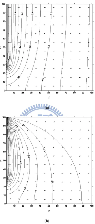
different radial distances as demonstrated in Figure 5(b) when S = 0.1. Figures 6(a) and y

6(b) illustrates the spatial flow pattern for S = 0 and 0.1 at y τ = 10

4 _{with the same}

parameter values as those to draw Figure 5. Apparently, the vertical flow occurs only near

the bottom edge of the well screen when the aquifer is confined. However, for unconfined

aquifers, the flow at free surface is almost vertical and obvious vertical flows occur near both

the top and bottom edges of the well. It demonstrates that the vertical flow in the unconfined

system is induced not only by the effect of partial penetration but also the effect of free

surface boundary.

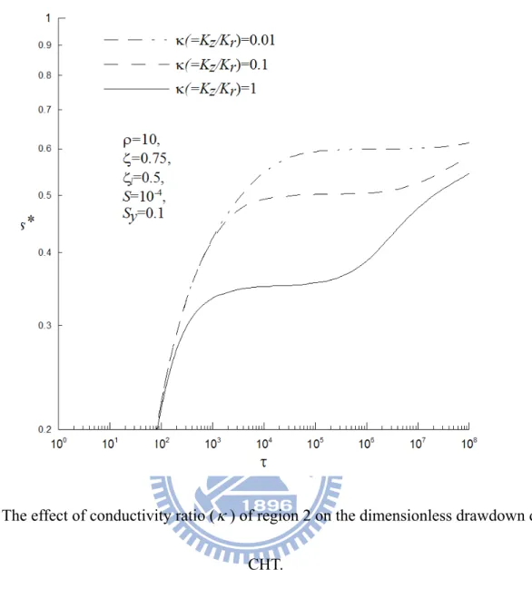
4.5 Effect of anisotropy

Figure 7 demonstrates the effect of the conductivity ratio κ (=Kz/Kr) on the

dimensionless drawdown during CHT. The vertical axis represents the dimensionless

drawdown and the horizontal axis represents the dimensionless time. The κ ranges from

2

10− to 1 with ₌₁₀−4

r

K m/min, β =100 , S =10−4, 1S_y =0. , and ζl =0.5. The

dimensionless drawdown decreases with increasing κ indicating that the vertical flow from

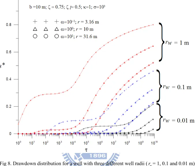
4.6 Influence of the well radius

Figure 8 illustrates the effect of the well radius on drawdown distribution in a 10 m thick

aquifer. The considered well radii are 1, 0.1 and 0.01 m with _{σ =10}3_{, ζ =0.75, 5=0.}

l ζ

and 1κ = . Drawdown is calculated at the distances of 3.16, 10, or 31.6 m from the

pumping well for α 10= -1_{, 1, and 10}1_{, respectively. The drawdown decreases with} increasing distance from pumping well for different r as demonstrated in Figures 2a-d. w

The drawdown increases with r for different value of w α , indicating that the well radius has

significant effect on the drawdown distribution.

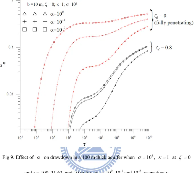
4.7 Effect of partially penetration

The effect of α on drawdown in the aquifer at ζ =0 when the well is fully (ζl =0) and

partially penetrating (ζl =0.8 ), is plotted in Figure 9 for

3

10 =

σ and κ =1. The

drawdown difference between the cases of full penetration and partial penetration decreases

with increasing α . It is reasonable that _α1/2 _{is directly proportional to the radial distance}

from the pumping well when the aquifer is isotropic and the partial penetration effect vanishes

when the radial distance goes large. Since α1/2 / κ

b

r = , it is proved that the radial

distance influenced by the partial penetration in unconfined aquifer under CHT is proportional

CHAPTER 5 CONCLUSIONS

A semi-analytical solution of the drawdown distribution is developed for CHT performed

in an unconfined aquifer with a partially penetrating well. The Laplace transforms and the

method of separation of variables are employed to derive the transient drawdown in the

Laplace domain for CHT. The Stehfest method is used to invert the solutions in

time-domain and the Shanks method is applied to accelerate convergence in evaluating the

infinite summations in the solution.

Large slopes of the drawdown distribution curves can be observed near the free surface

boundary and the edge of the screen, which indicates that the vertical groundwater flows

occur at these two areas. The dimensionless drawdown decreases with increasing S but y

increases with the length of well screen. For different r , the drawdown decreases with the w

increase of radial distance from pumping well and it might produce large error in drawdown if

assuming the radius of pumping well is infinitesimal.

The present solution can be used for describing the transient drawdown distribution or

investigating the effects of specific yield and conductivity ratio on the drawdown distribution

in unconfined aquifers. In addition, the present solution can reduce to the solution for a fully

penetrating well in either confined or unconfined aquifers under CHT.

APPENDIX A

The dimensionless governing equations of Eqs. (1) and (3) can be expressed as l w s s s s _{ρ ζ ζ} τ ζ α ρ ρ ρ ∂ ≤ ≤ ≤ ≤ ∂ = ∂ ∂ + ∂ ∂ + ∂ ∂ 0 , 1 0 , 1 * 1 2 * 1 2 * 1 2 * 1 2 (A1) and 1 0 , 1 , 1 * 2 2 * 2 2 * 2 2 * 2 2 ≤ ≤ ∞ < ≤ ∂ ∂ = ∂ ∂ + ∂ ∂ + ∂ ∂ _{ρ ζ} τ ζ α ρ ρ ρ s s s s w (A2) The dimensionless initial conditions for regions 1 and 2 are

0 ) 0 , , ( ) 0 , , ( * 2 * 1 ρ ζ =s ρ ζ = s (A3)

and the boundary conditions at the bottom and top of the aquifer for regions 1 and 2 in terms

of dimensionless form can be written as

0 ) , , ( ) , , ( 0 * 2 0 * 1 ₌ ∂ ∂ = ∂ ∂ = = ζ ζ ζ τ ζ ρ ζ τ ζ ρ s s (A4) 1 0 , 0 ) , , ( * 1 _{= ≤ ≤} ∂ ∂ = ρ ζ τ ζ ρ ζ ζ l s (A5) and ∞ < ≤ ∂ ∂ − = ∂ ∂ = = ρ τ τ ζ ρ α σ ζ τ ζ ρ ζ ζ 1 , ) , , ( ) , , ( 1 * 2 1 * 2 s s w (A6)

The dimensionless boundary conditions at ρ = 0 and infinity are respectively written as

l s _{ζ ζ} ρ τ ζ < < = ∂ ∂ 0 , 0 ) , , 0 ( * 1 _(A7) 0 ) , , ( * 2 ∞ ζ τ = s (A8)

The dimensionless boundary condition along the screen is expressed as

0 , 1 , 1 ) , , 1 ( * 2 ζ τ = ζl <ζ < τ > s (A9)

0 , 0 ), , , 1 ( ) , , 1 ( * 2 * 1 ζ τ =s ζ τ <ζ <ζl τ > s (A10) and 0 , 0 , ) , , ( ) , , ( 1 1 * 2 * 1 _{< < >} ∂ ∂ = ∂ ∂ = = τ ζ ζ ρ τ ζ ρ ρ τ ζ ρ ρ ρ l s s (A11)

The Laplace transform is defined as:

∫

∞ − = → = 0 * * 1 * 1 ( , , ) [ ( , , ); ] ( , , ) ~ _{ρ ζ ρ ζ τ τ ρ ζ τ} τ _τ d e s p s L p s _p p (A12)

where )~s₁*(ρ,ζ,p is the dimensionless drawdown in Laplace domain. The solution for the

dimensionless drawdown solutions can be obtained by taking Laplace transforms of

governing equations Eqs. (A1) to (A2) using the initial condition (A3) and the results are

* 1 2 * 1 2 * 1 2 * 1 2 ~ ~ ~ 1 ~ s p s s s w = ∂ ∂ + ∂ ∂ + ∂ ∂ ζ α ρ ρ ρ , 0≤ρ ≤1, 0≤ζ ≤ζl (A13) and * 2 2 * 2 2 * 2 2 * 2 2 ~ ~ ~ 1 ~ s p s s s w = ∂ ∂ + ∂ ∂ + ∂ ∂ ζ α ρ ρ ρ , 1≤ρ <∞, 0≤ζ ≤1 (A14) The transformed boundary conditions at the bottom and top of the aquifer for regions 1 and 2

can be written as 0 ) , , ( ~ ) , , ( ~ 0 * 2 0 * 1 ₌ ∂ ∂ = ∂ ∂ = = ζ ζ ζ ζ ρ ζ ζ ρ p s p s (A15) 1 0 , 0 ) , , ( ~* 1 _{= < <} ∂ ∂ = ρ ζ ζ ρ ζ ζ l p s (A16) and ) , 1 , ( ~ ) , , ( ~ * 2 1 * 2 p _{p s p} s w = ⋅ ⋅ − = ∂ ∂ = ζ ρ α σ ζ ζ ρ ζ (A17)

In the same fashion, the transformed boundary conditions at ρ= 0 and ∞ are l p s _{ζ ζ} ρ ζ < < = ∂ ∂ 0 , 0 ) , , 0 ( ~* 1 _(A18) and 0 ) , , ( ~* 2 ∞ p = s ζ (A19)

After taking the Laplace transform, the boundary condition along the well screen is

0 , 1 , 1 ) , , 1 ( ~* 2 ζ = ζl <ζ < τ > p p s (A20)

and continuity conditions become

l p s p s (1,ζ, )=~ (1,ζ, ), 0<ζ <ζ ~ * 2 * 1 (A21) and l p s p s _{ζ ζ} ρ ζ ρ ρ ζ ρ ρ ρ < < ∂ ∂ = ∂ ∂ = = 0 , ) , , ( ~ ) , , ( ~ 1 1 * 2 * 1 _(A22) Assume that * 1 ~

s and ~s₂* are the product of two distinct functions, i.e.,

) , ( ) , ( ) , , ( ~ 1 1 * 1 p F p G p s ρ ζ = ρ ζ and s~₂*(ρ,ζ,p)=F₂(ρ,p)G₂(ζ,p) , respectively.

Equations (A13) and (A14) can be, respectively, transformed as

1 1 21 2 1 1 1 21 2 1 1 G pF G F F G F G _w = ∂ ∂ + ∂ ∂ + ∂ ∂ ζ α ρ ρ ρ (A23) and 2 2 22 2 2 2 2 22 2 2 1 G pF G F F G F G _w = ∂ ∂ + ∂ ∂ + ∂ ∂ ζ α ρ ρ ρ (A24) Dividing throughout Equations (A23) and (A24) by F₁G₁ and F₂G₂, respectively, Equations

0 1 1 21 2 = + ∂ ∂ G G w m α ω ζ (A25)

[

]

0 1 1 1 1 21 2 = + − ∂ ∂ + ∂ ∂ F p F F m ω ρ ρ ρ (A26) and 0 2 2 22 2 = + ∂ ∂ G G w n α ω ζ (A27)

[

]

0 1 2 2 2 22 2 = + − ∂ ∂ + ∂ ∂ F p F F n ω ρ ρ ρ (A28) where ω1m and ω2n are separation constants.

The solutions of (A25) and (A27) subject to the boundary in (A15) are respectively

) cos( ) ( ) , ( _{1 1} 1 ζ p am p mζ G = Ω (A29) and ) cos( ) ( ) , ( _{2 2} 2 ζ p a n p nζ G = Ω (A30)

where Ω =1m ω1m/αw and Ω =2n ω2n/αw , )a1m(p and a2n(p) are constants with

respect to p . In addition, substituting (A29) into (A16) yields the following equation

0 )

sin(Ω₁mζl = (A31)

The eigenvalues Ω in Equation (A29) can then determined by solving Equation (A31) and 1m

the result is , 1 l m m ζ π = Ω m = 0, 1, 2, … (A32)

Similarly, substituting (A30) into (A17) gives the following equation

) cos( ) sin( _{2 2} 2 n w n n Ω = p Ω Ω α σ , n= 0, 1, 2,… (A33)

The general solutions of (A26) and (A28) are respectively ) ( ) ( ) ( ) ( ) , ( _{1 0 1 1 0 1} 1 ρ p cm p I p ωmρ dm p K p ωmρ F = + + + (A34) and ) ( ) ( ) ( ) ( ) , ( _{2 0 2 2 0 2} 2 ρ p c n p I p ω nρ d n p K p ω nρ F = + + + (A35)

where )c₁m(p , )d1m(p , )c2n(p and d2n(p) are constants.

Then, substituting (A34) into (A18) and (A35) into (A19), respectively, yields

) 0 ( ) ( ) 0 ( ) ( ) , ( 1 1 1 1 1 0 K p d I p c p F m m − = ∂ ∂ = ρ ρ ρ (A36) and ) ( ) ( ) ( ) ( ) , ( _{2 0 2 0} 2 ∞ p =c p I ∞ +d p K ∞ F n n (A37)

where )c₁m(p and d2n(p) are constants. Note that d1m(p) and c2n(p) equal zero

because K₁(0) and I₀(∞) are, respectively, equal to infinity. The solutions of (A26) and (A28) are respectively

) ( ) ( ) , ( _{1 0 1} 1 ρ p cm p I p ωmρ F = + (A38) and ) ( ) ( ) , ( _{2 0 2} 2 ρ p d n p K p ω nρ F = + (A39)

The product of (A29) and (A38) gives the general solution of Equation (A23) as

) cos( ) ( ) ( ) , , ( ~ 1 1 0 1 1 * _{ρ ζ ω ρ ζ} m m m m p A p I p s = + Ω m = 0, 1, 2, … (A40)

) cos( ) ( ) ( ) , , ( ~ 2 2 0 2 2 * _{ρ ζ ω ρ ζ} n n n n p A p K p s = + Ω n= 0, 1, 2,… (A41)

where )A₂n(p is the product of a2n(p) and d2n(p). Accordingly, the linear combination of

all the m’s solutions yields the complete solution for ~*( , , )

1 p s ρ ζ

∑

∞ = Ω + = 0 1 1 0 1 * 1 ( , , ) ( ) ( )cos( ) ~ m m m m p I p A p s ρ ζ ω ρ ζ (A42)

Similarly, the complete solution for ~*( , , )

2 p s ρ ζ can be obtained as

∑

∞ = Ω + = 0 2 2 0 2 * 2 ( , , ) ( ) ( )cos( ) ~ n n n n p K p A p s ρ ζ ω ρ ζ (A43)

The coefficients A₁m(p) and A2n(p) are unknowns at this stage and can be solved from the

following equation obtained by substituting (A42) and (A43) into (A21) and (A20),

respectively, as 1 , 1 ) cos( ) ( ) ( 0 2 2 0 2 + Ω = < <

∑

∞ = ζ ζ ζ ω l n n n n p p K p A (A44) and

∑

∑

∞ = ∞ = < < Ω + = Ω + 0 2 2 0 2 0 1 1 0 1 ( ) ( )cos( ) ( ) ( )cos( ), 0 n l n n n m m m m p I p A p K p A ω ζ ω ζ ζ ζ (A45)

Equations (A40) and (A41) are organized and expressed as

∑

∑

∞ = ∞ = < < Ω + = Ω + 0 1 1 0 1 0 2 2 0 2 ( ) ( )cos( ) ( ) ( )cos( ), 0 m l m m m n n n n p K p A p I p A ω ζ ω ζ ζ ζ 1 , 1 _{< <} = ζl ζ p (A46) In order to obtain concise solutions, we further define A₂n (p)=A₂n(p)K₀( p+ω₂n)

′ _and ) ( ) ( ) ( _{1 0 1} 1m p Am p I p m

A ′ = +ω and (A42) can be rewritten as

1 0 ), ( ) cos( ) ( ' 0 2 2 Ω = < <

∑

∞ = ζ ζ ζ f p A n n n (A47) where

∑

∞ = < < Ω ′ = 0 1 1 ( )cos( ), 0 ) ( m l m m p A f ζ ζ ζ ζ 1 , 1 _{< <} = ζl ζ p (A48) The term on the left-hand side (LHS) of Eq. (A47) is a half-range Fourier cosine series of

the function on the right-hand side (RHS) of Eq. (A47) for the region 0<ζ <1. The

coefficient A_2n′(p) can then be obtained from the properties of Fourier series as

∫

∫

Ω Ω = ′ 1 0 2 2 1 0 2 2 ) ( cos ) ( ) cos( ) ( ζ ζ ζ ζ ζ d d f p A n n n (A49)

Carrying out the integration in (A49) and simplifying the result yields the coefficient A₂n'(p)

as expressed in Eq. (17).

Similarly, substituting (A42) and (A43) into (A22), one can obtain

∑

∑

∞ = ∞ = Ω + + + ′ − = Ω ′ 0 _{0 2} 2 2 1 2 2 0 1 1 ) cos( ) ( ) ( ) ( ) cos( ) ( n n n n n n m m m p K p K p p A p A ζ ω ω ω ζ , 0<ζ <ζ_l (A50)

From (A50), the coefficient A_1m′(p) can be determined as Equation (15).

Accordingly, based on the coefficients A₁m'(p) and A2n'(p), the complete solution for

* 1

~

APPENDIX B

Simplification of Eqs. (15) and (16) to the case of fully penetrating well in unconfined

Letting 0ζl = in Eqs. (16) and (17), the drawdown solution of Eq. (14) in region 1 is equal

to zero and the Laplace-domain solution in Eq. (15) for dimensionless drawdown in region 2

pumping from a fully penetrating well in unconfined aquifers can be expressed as

) cos( ) ( ) ( 2 ) 2 sin( ) sin( 4 ) , , ( ~ 2 2 0 2 0 2 2 2 0 * 2 _ω ζ ρ ω ζ ρ _n n n n n n n K p p K p p s Ω + ⋅ + ⎥ ⎦ ⎤ ⎢ ⎣ ⎡ Ω + Ω Ω =

∑

∞ = (B1)

Considering the skin effect in pumping system, Chen and Chang (2003) developed a

Laplace-domain solution for describing the flow in an unconfined aquifer with pumping from

a fully penetrating well under constant-head test. The solution is expressed as

⎭ ⎬ ⎫ ⎩ ⎨ ⎧ + ⋅ =

∑

∞ = − ) cos( ) cos( ) ( ) ( ) ( 2 ) , , ( 1 0 1 0 1 n n n n n k n n n D K S K K p L h ε λ ζ ε χ χ χ ρ χ τ ζ ρ (B2) β σ ε εtan( )= p (B3) ) / ( / 1 2 p p β ε_n β σ σ λ = + + (B4) where ( / )( 2/ 2) b r K Kz r w = β , ρ =r /rw , σ =Sy/S , 2 n n p βε χ = + , ζ =z /b , ) /( ) ( 2 S r Tt _w =

τ , ε_n is nth positive root of Eq. (B3), S is skin factor, p is Laplace _k

transform parameter and −1{}

L is the Laplace inversion operator.

If skin effect is negligible (Sk =0), Eq. (B2) can be rearranged as

⎭ ⎬ ⎫ ⎩ ⎨ ⎧ ⋅ =

∑

∞ = − ) cos( ) cos( ) ( ) ( 2 ) , , ( 1 0 0 1 n n n n n n D K K p L h ε λ ζ ε χ ρ χ τ ζ ρ (B5)

Since Eqs. (B1) and (B5) are both used for calculating the dimensionless drawdown in

identical to Eq. (B5).

Some definitions of variable in Eq. (B5) are different from that in Eq. (B1) and the

relations are αw =β, Ω2n =εn and p+ω2n =χn. Eq. (B5) can be thus rearranged as

⎪⎭ ⎪ ⎬ ⎫ ⎪⎩ ⎪ ⎨ ⎧ Ω Ω + ⋅ + =

∑

∞ = − ) cos( ) cos( ) ( ) ( 2 ) , , ( 2 2 1 _{0 2} 2 0 1 n n n n _n n D p K p K p L h λ ζ ω ρ ω τ ζ ρ (B6)

Substituting (B3) into Eq. (4), one can obtain

) tan( ) tan( 1 2 2 2 2 n n n n n _Ω Ω + Ω Ω + = λ (B7)

In addition, substituting (B6) into the term on the left-hand side (LHS) of Eq. (B5) results

in ) cos( ) tan( ) tan( 1 1 ) cos( 1 2 2 2 2 2 2 n n n n n n n _Ω ⎥ ⎦ ⎤ ⎢ ⎣ ⎡ Ω Ω + Ω Ω + = Ω λ (B8)

Using the tangent relation (i.e.,tan(ϑ)=sin(ϑ)/cos(ϑ)), the denominator on the right-hand

side (RHS) of Eq. (B8) can be expressed as

) sin( ) ( cos ) sin( ) cos( 1 ) cos( ) tan( ) tan( 1 1 2 2 2 2 2 2 2 2 2 2 2 2 n n n n n n n n n n n Ω Ω Ω + Ω Ω + Ω = Ω ⎥ ⎦ ⎤ ⎢ ⎣ ⎡ Ω Ω + Ω Ω + (B9)

The RHS in Eq. (B8) can be further written as

⎥ ⎦ ⎤ ⎢ ⎣ ⎡ Ω Ω + Ω Ω + Ω = Ω Ω Ω + Ω Ω + Ω ) sin( ) ( cos ) sin( ) cos( 1 ) sin( ) ( cos ) sin( ) cos( 1 2 2 2 2 2 2 2 2 2 2 2 2 2 n n n n n n n n n n n (B10)

Eq. (B10) can be simplified using the triangle relationship (i.e., sin2(_ϑ)₊cos2(_ϑ)₌1_{) as}

) sin( ) cos( 1 ) sin( ) ( cos ) sin( ) cos( 1 2 2 2 2 2 2 2 2 2 n n n n n n n n Ω Ω + Ω = ⎥ ⎦ ⎤ ⎢ ⎣ ⎡ Ω Ω + Ω Ω + Ω (B11)

n n n n n n 2 2 2 2 2 2 sin(2 ) 2 ) sin( 2 ) sin( ) cos( 1 Ω + Ω Ω = Ω Ω + Ω (B12)

From Eq. (B7) to (B11), the following relation is established

n n n n n 2 2 2 2 ) 2 sin( ) sin( 2 ) cos( 1 Ω + Ω Ω = ε λ (B13) Furthermore, base on Ω2n =εn and Eqs. (B6)-(B13), one can easily prove that Eq. (B1)

APPENDIX C

The Laplace-domain solution of Eq. (15) in region 2 for describing the flow due to pumping

from a fully penetrating well in confined aquifers can be expressed as

) cos( ) ( ) ( 2 ) 2 sin( ) sin( 4 ) , , ( ~ 2 2 0 2 0 2 2 2 0 * 2 _ω ζ ρ ω ζ ρ _n n n n n n n K p p K p p s Ω + ⋅ + ⎥ ⎦ ⎤ ⎢ ⎣ ⎡ Ω + Ω Ω =

∑

∞ = (C1)

Substituting σ =0 (i.e., Sy =0 for confined aquifers) into Eq. (A33), one can obtain ... , 2 , 1 , 0 2 = = Ω n nπ n (C2)

Substituting Eq. (C2) into Eq. (C1) and using L'Hospital's rule, Eq. (C1) is simplified as

) ( ) ( 1 ) , , ( ~ 0 0 * 2 p K p K p p s ρ ζ = ⋅ρ (C3)

The non-dimensional form of Eq. (C3) is

) ( ) ( ' 1 ) , , ( ~ 2 0 2 0 2 p K r S K r r p K r S K p s p s r w s w r w s w ′ ⋅ ′ = ζ ρ _(C4) where p′=(S_sr_w2/K_r)p.

Eq. (C4) is further simplified as

) ( ) ( ' 1 ) , , ( ~ 0 0 2 w r s r s w r p K S K r p K S K p s p s ′ ′ = ζ ρ (C5)

Assuming the aquifer is confined, homogeneous and isotropic, the solution in Eq. (C5) is

identical to the Laplace-domain solution in Hantush (1964) written as

)

(

)

(

)

,

(

0 0 w w

r

pK

r

K

s

p

r

s

⋅

⋅

⋅

=

λ

λ

(C6) where λ= (p⋅S_s)/K .

REFERENCES

Abdul, A. S. “A new pumping strategy for petroleum product recovery from contaminated

hydrogeologic systems: Laboratory and field evaluations” Ground Water Monit. Rem. 12,

pp.105-114, 1992.

Batu, V. “Aquifer hydraulics: a comprehensive guide to hydrogeologic data analysis” John

Wiley & Sons Inc., New York, 1998.

Boulton, N. S. “Unsteady radial flow to a pumped well allowing for delayed yield from

storage” Intern. Assoc. Sci. Hydrol.,Rome. Pubi., 37, pp. 472-477, 1954.

Chen, C. S., and Chang, C. C. “Well hydraulics theory and data analysis of the constant head

test in an unconfined aquifer with the skin effect” Water Resour. Res.,39(5), pp.

1121-1135, 2003.

Cheng, A. H.-D., and Siduruk, P. “Approximate Inversion of the Laplace Transform” The

Mathematic Journal, 4 (2), pp.76-82, 1994.

Crump, K.S., “Numerical inversion of Laplace trans- forms using a Fourier

series approximation” J. Assoc. Comput. Mach.,23(1), pp. 89-96, 1976.

Chang, Y. C., and Yeh, H. D. “New solutions to the constant-head test performed at a

partially penetrating well” J. Hydrology, 369, pp. 90-97, 2009.

pp. 640-651, 2010.

Chang, Y. C., Yeh, H. D. and Chen, G. Y. “Transient solution for radial two-zone flow in

unconfined aquifers under constant-head test” Hydrological Processes, 24, pp.

1496-1503, 2010.

Hantush, M.S. “Hydraulics of wells” in Advances in Hydroscience, vol. 1, V.T. Chow, eds.,

Academic. San Diego. Calf., pp. 281-432, 1964.

Hiller, C. K., and Levy, B. S. “Estimation of aquifer diffusivity from analysis of constant-head

pumping test data” Ground Water, 32(1), pp. 47–52. 1994.

Javandel, I., Zaghi, N. “Analysis of flow to an extended fully penetrating well” Water Resour.

Res., 11(1), pp. 1059-164, 1975.

Jones, L., Lemar T., and Tsai, C. T. “Results of two pumping tests in Wisconsin age

weathered till in Iowa” Ground Water, 30(4), pp. 529-538, 1992.

Jones, L. “A comparison of pumping and slug tests for estimating the hydraulic conductivity

of unweathered Wisconsin age till in Iowa” Ground Water, 31(6), pp. 896-904, 1993.

Kirkham, D. “Exact theory of flow into a partially penetrating well” J. Geophys. Res., 64(9),

pp. 1317-1327, 1959.

Malama, B., Kuhlman, K.L., Barrash, W. “Semi-analytical solutions for flow in leaky

unconfined aquifer-aquitard systems” J. Hydrology, 346(1-2), pp. 59-68, 2007.

unconfined aquifer toward a partially penetrating pumping well” J. Hydrology, 356(1-2),

pp. 234-244, 2008.

Malama, B., Kuhlman, K. L., Revil A. “A semi-analytical solution for transient streaming

potentials associated with confined aquifer pumping tests” Geophysical Journal

International, 176(3), pp. 1007-1016, 2009.

Malama, B., Kuhlman, K. L., Revil, A. “Theory of transient streaming potentials associated

with axial-symmetric flow in unconfined aquifers” Geophysical Journal International,

179(2), pp.990-1003, 2009.

Mishra, S., and Guyonnet, D. “Analysis of observation-well response during constant-head

testing” Ground Water, 30(4), pp. 523–528, 1992.

Moench, A. F. “Flow to a well of finite diameter in a homogeneous, anisotropic water table

aquifer” Water Resour. Res.. 33(6), pp. 1397-1407, 1997.

Murdoch, L. D., and Franco, J. “The analysis of constant drawdown wells using instantaneous

source functions” Water Resour. Res., 30(1), pp. 117-127, 1994.

Neuman, S. P. “Theory of flow in unconfined aquifers considering delayed response of the

water table” Water Resour. Res., 8(4), pp. 1031-1045, 1972.

Neuman, S. P. “Effects of partial penetration on flow in unconfined aquifers considering

flow to a partially penetrating well in a phreatic aquifer” Adv. Water Resour., 31, pp.

383-398, 2008.

Peng, H. Y., Yeh, H. D. and Yang, S. Y. “Improved numerical evaluation of the radial

groundwater flow equation” Adv. Water Resour., 25(6), pp. 663-675, 2002.

Renard, P. “Approximate discharge for constant head test with recharging boundary” Ground

Water,. 43, pp. 439-442, 2005.

Rizzo, E., Suski, B., Revil, A., Straface, S., and Troisi, S. “Self-potential signals associated

with pumping tests experiments” Journal of Geophysical Research-Solid Earth,

109(B10203), 2004.

Shanks, D. “Non-linear transformations of divergent and slowly convergent sequence” J.

Math. Phys., 34, pp. 1-42, 1955.

Singh SK. “Simple approximation of well function for constant drawdown variable discharge

artesian wells” J. Irrigation and Drainage Engineering 133(3), pp. 282–285, 2007.

Stehfest, H. “Numerical inversion of Laplace transforms” Comm. ACM 13, pp. 47-49, 1970.

Theis, C.V. “The relation between the lowering of the piezometric surface and the rate and

duration of discharge of a well using groundwater storage”, Am. Geophys. Union Trans.,

16, pp. 519-524, 1935.

Tartakovsky, G. D., and Neuman, S. P. “Three-dimensional saturated-unsaturated flow with

Water Resour. Res., 43, W01410, doi:10.1029/2006WR005153, 2007.

Uraiet, A. A., and Raghavan, R. “Unsteady flow to a well producing at a constant pressure” J.

Pet. Technol., 32(10), pp. 1803-1812, 1980.

Yang, S. Y., and Yeh, H. D. “Solution for flow rates across the wellbore in a two-zone

confined aquifer” J. Hydraul. Eng., ASCE, 128(2), pp. 175-183, 2002.

Yang, S. Y., and Yeh, H. D. “Laplace-domain solutions for radial two-zone flow equations

under the conditions of constant-head and partially penetrating well” J. Hydraul. Eng.,

ASCE, 131(3), pp. 209-216, 2005.

Wilkinson, W. B. “Constant head in situ permeability tests in clay strata” Geotechnique, 18,

pp. 172-194, 1968.

Wynn, P. “On a device for computing the em(Sn) transformation” Math. Tables Aids Compyt.,

(a) (b)

(c) (d)

Fig 2. The dimensionless drawdown distributions at τ = (a) 1 , (b) 102 , (c) 104 , and (d)

Fig 4. The dimensionless drawdown distributions at the well screen extended from ζ = to ζl

β

(a)

(b)

Fig 5. Relationship for dimensionless drawdown versus dimensionless time with ζ =50, 75,

(a)

(b)

Fig 6. Spatial flow pattern in an unconfined aquifer with a partially penetrating well for κ =1,

100 = β , 25ζl = , 4 10− =

Fig 7. The effect of conductivity ratio (κ) of region 2 on the dimensionless drawdown during

Fig 8. Drawdown distribution for a well with three different well radii (r = 1, 0.1 and 0.01 m) w

with _{σ =10}3_{, ζ =0.75, 5=0.}

l

Fig 9. Effect of α on drawdown in a 100 m thick aquifer when _{σ =10}3_{, 1κ = at ζ =0}