國 立 交 通 大 學
經營管理研究所
碩 士 論 文
波動成分情緒指標與雜訊交易者風險
Volatility Components Sentiment Indices and
Noise Trader Risk
研 究 生:郭念青
指導教授:周雨田 教授
波動成分情緒指標與雜訊交易者風險
Volatility Components Sentiment Indices and Noise Trader
Risk
研 究 生︰郭念青 Student︰Nien-Ching Kuo 指導教授︰周雨田 博士 Advisor︰Dr. Ray Yeu-Tien Chou
國立交通大學
經營管理研究所
碩士論文
A Thesis
Submitted to Institute of Business and Management College of Management
National Chiao Tung University in Partial Fulfillment of the Requirements
for the Degree of
Master of Business Administration
June 2008
Taipei, Taiwan, Republic of China 中華民國 九十七 年 六 月
波動成分情緒指標與雜訊交易者風險
研究生:郭念青 指導教授:周雨田博士
國立交通大學經營管理研究所碩士班
摘 要
我們使用 GJR-GARCH 和七種情緒指標來檢驗 De Long 等(1990a)所提出雜訊交易者
風險在條件波動和超額報酬上的影響。我們發現情緒是一個解釋股票超額報酬和條件波
動很顯著的因子。情緒的變化量對於條件波動和超額報酬有很顯著的影響。PCO、AAII、
II 和 IPON 可以用來預測未來的報酬,而 ARMS、PCO、PCV、AAII 和 IPON 可以預測
報酬波動。看漲的情緒會使得條件波動向下修正,而看跌的情緒則會使波動向上爬升。
此外,我們使用 Component GARCH 檢測雜訊交易者風險在長期和短期的情形。我們發
現情緒在短期波動的影響比長期波動來的大且顯著。
Volatility components sentiment indices and noise trader risk
Student: Nien-Ching Kuo Advisor: Dr. Ray Yeu-Tien Chou
Institute of Business and Management National Chiao Tung University
ABSTRACT
Using seven sentiment indices, we employ a GJR-GARCH specification to test the impact of
noise trader risk on both the formation of conditional volatility and expected return as
suggested by De Long et al. (1990a). Our main findings suggest that sentiment is a significant
factor in explaining equity excess returns and conditional volatility. We find that the
magnitude of shifts in sentiment has a significant impact on the formation of conditional
volatility of returns and expected returns. PCO, AAII, II, and IPON can be used to forecast the
future returns and ARMS, PCO, PCV, AAII, and IPON are good proxy to forecast the
volatility of returns. Bullish (bearish) shifts in sentiment lead to downward (upward) revisions
in the volatility of returns. In addition, we try to use the component GARCH to divide the
noise trader risk into two components which are the transitory component and the permanent
component. We find that effect of sentiment in the transitory component is larger and more
significant than in the permanent component.
誌 謝
本論文可以完成,首先感謝我的指導教授周雨田博士,老師鼓勵同學尋找自己喜歡 的題目,在老師細心的教導下,使我得以一窺財務計量領域的深奧,不時的討論並指點 我正確的方向,使我在這兩年獲益良多。老師對學問的嚴謹更是我輩學習的典範。也要 感謝口試委員丁承教授、周冠男教授和涂登才教授仔細的閱讀我的論文,提出非常多寶 貴的意見,讓我了解更多論文的技巧,也讓這篇論文增色不少。 在 尋 找 論 文 資 料 的 過 程 發 生 很 多 困 難,感 謝 王 耀 輝 老 師 的 幫 忙,指 點 資 料 來 源。當 然 也 要 感 謝 母 親 出 錢 購 買 論 文 資 料。劉 炳 麟 學 長 也 常 常 參 與 我 們 的 討 論 , 給 我 很 多 實 用 的 建 議 。 當 然 同 門 的 夥 伴 們 也 不 可 少 , 感 謝 致 宏 、 維 苡 、 文 元 在 資 料 蒐 集 上 的 幫 忙 和 平 時 的 共 患 難 互 相 加 油 打 氣 , 也 感 謝 志 豪 、 安 婷 、 志 勤 、 美 娟 和 士 漢 學 長 平 時 的 照 顧 。 感 謝 瓊 文 對 於 我 論 文 格 式 上 的 幫 忙 , 與 聽 我 吐 苦 水 。 當 然 還 有 不 管 是 高 中 、 大 學 、 或 是 研 究 所 的 好 朋 友 們 , 你 們 的 鼓 勵 是 我 最 大 的 動 力 。 兩年裡的日子,研究室裡共同的生活點滴,學術上的討論、言不及義的閒扯、趕報 告拼考試的革命情感,常常搞到三更半夜才回家(也不知道在幹嘛),真的讓人覺得很溫 馨,感謝眾位學長姐、同學、學弟妹,你們的陪伴讓兩年的研究生活變得絢麗多彩。最 後,感謝我的家人對我的包容與支持,在我求學生涯無後顧之憂,能夠專心的求學。謹 以此文獻給我摯愛的雙親。Table of contents
摘 要 ... i ABSTRACT ... ii 誌 謝 ...iii Table of contents ... iv List of Tables ... v List of Figures ... vi 1. Introduction ... 1 2. Literature Review ... 5 3 Data ... 93.1. Direct sentiment measures... 9
3.2. Indirect sentiment measures ... 10
3.2.1. Market performance ... 10
3.2.2. Derivatives variables ... 11
3.2.3. Other sentiment proxies... 12
3.3. Sample period and stock return proxies ... 12
4. Empirical design ... 14
4.1. Hypotheses ... 14
4.2. The generalized autoregressive conditional heteroscedasticity model... 15
4.2.1. The GJR-GARCH model ... 16
4.2.2. The component GARCH ... 18
5. Results... 20
5.1. Summary statistics... 20
5.2. Estimated GJR-GARCH results ... 23
5.3. Estimated Component GARCH results ... 29
6. Conclusion ... 31
References ... 36
List of Tables
Table 1 Correlation matrix for the weekly American Association of Individual Investors
sentiment index (bullish percentage) and Investors’ Intelligence sentiment index (bullish percentage)………...…..39
Table 2 Summary statistics of return, excess return, and sentiment index, for daily data,
8/22/1996-12/31/2007……….…40
Table 3 Summary statistics of return, excess return, and sentiment index, for weekly data,
7/24/1987-12/31/2007……….41
Table 4 Summary statistics of return, excess return, and sentiment index, for monthly data,
2/01/1971-12/31/2006……….………42
Table 5 Estimation of the GJR-GARCH base model without sentiment index for daily,
weekly, and monthly excess return………...43
Table 6 Estimation of the GJR-GARCH model with sentiment index for daily excess
returns……….44
Table 7 Estimation of the GJR-GARCH model with sentiment index for weekly excess
returns……….45
Table 8 Estimation of the GJR-GARCH model with sentiment index for monthly excess
returns……….46
Table 9 Estimation of the Components GARCH model with sentiment index for daily
excess returns…...………...47
Table 10 Estimation of the Components GARCH model with sentiment index for weekly
excess returns………..………48
Table 11 Estimation of the Components GARCH model with sentiment index for monthly
List of Figures
Figure 1 Direct sentiment measures……….50
Figure 2 Market performance measures……….………51
Figure 3 Derivatives variable measures……….…...……...52
Figure 4 Other sentiment proxies……….………53
Figure 5 Daily stock indices……….…………54
Figure 6 Weekly stock indices……….………….56
Figure 7 Monthly stock indices……….………...58
Figure 8 Average three-month T-Bill yield………..60
1. Introduction
For decades, the success and popularity of the efficient market hypothesis (EMH) lies in its
ability to explain the lack of predictability in liquid asset returns, meanwhile traditional
“search for value” is clashed by many finance practitioners. More recent analysis has
discussed how such traders acting sentiment might induce systematic risk and affect asset
prices in equilibrium. For example, as the noise trader models of De Long, Shleifer, Summers,
and Waldmann (1990a; 1990b) suggest that if informed arbitrageurs know that prices may
diverge further away from fundamentals before they converge closer, they may take smaller
positions when betting against mispricing. If these uninformed noise traders base their trading
decisions on sentiment, sentiment may have predictive power for asset price behavior. The
noise trader model of De Long, Shleifer, Summers, and Waldmann (1990a) has motivated
empirical attempts to substantiate the proposition that noise trader risks influence price
formation.
Most papers test whether sentiment can predict returns or volatility. They attempt to
explain this correlative relationship through the role of noise traders whose changes in
sentiment can influence subsequent returns and volatility. If it is true, we can use sentiment as
an indicator to forecast not only the returns but volatility as well. Many papers in the past
have used sentiment to forecast return or volatility, but rarely both at the same time.
The model of De Long, Shleifer, Summers, and Waldmann (1990a) predicts that the
direction and magnitude if changes in noise trader sentiment are relevant in asset pricing, the
subsequent empirical testing focused on the impact of sentiment either on the mean or
variance in asset returns alone, such testing are mispecified and at best can only be considered
as incomplete. The “price-pressure” and “hold-more” effects capture the impact of noise
“Friedman” and “create-space” effects reflect the impact of noise trading on excess returns
associated with the influence of the magnitude of sentiment changes on the future volatility of
returns.
The “hold-more” effect implies that noise traders’ increased holdings of risky assets when
their sentiment becomes more bullish raises market risk and thereby increases expected
returns; and vice versa, when they are bearish. However, noise traders overreact to good and
bad news. Asset prices are either too high or too low depending on where noise traders are on
average optimistic or pessimistic. Such overreaction lowers expected returns. This
“price-pressure” effects and market returns will correlate with changes in investor sentiment
and the direction of the correlation depends on which effect dominates.
In addition, the magnitude of the changes in perceptions about the asset’s risk by noise
traders associated with their shifts in sentiment also impact expected returns. Noise traders
usually have poor market timing because of their tendency to trade together with other noise
traders. Their capital losses are larger due to poor market timing and the magnitude of losses
regards the magnitude of the change in their misperceptions. The Friedman effect implies that
this changes result in higher market risk and lower expected returns. There is an adverse
impact that the Friedman effect has on expected returns depending on the “space” the noise
trading creates. A rise in noise traders’ misperceptions increases price uncertainty and crowds
out risk-averse informed investors. Therefore, the greater is the proportion of noise trading,
the higher will be expected returns.
Lee, Jiang, and Indro (2002) employ a generalized autoregressive conditional
heteroscedasticity (GARCH) in-mean model (Engle, 1982; Bollerslev, 1986; Engle, Lilien,
and Robins, 1987) to show that both the conditional volatility and excess returns are affected
by investor sentiment. In this paper, we also use a GJR-GARCH in-mean (Glosten,
model which includes contemporaneous shifts in investor sentiment within the mean equation,
while our model includes lagged shifts in investor sentiment in the mean equation.
We examine the relationship between volatility of market excess returns, excess returns,
and investor sentiment for three different market indices, the DOW Jones Industrial Average
(DJIA), the Standard and Poor’s 500 (S&P500) and the NASDAQ. In this paper, we use a lot
of sentiment indices to proxy the noise traders’ sentiment. For the daily data, we use the OEX
put-call trading volume ratio (PCV), the OEX put-call open interest ratio (PCO), and the
ARMS index for NYSE as the sentiment indices. For weekly data, we use the bullish
percentage of sentiment indices of Investors’ Intelligence (II) and the American Association
of Individual Investors (AAII). And for monthly data, we use the initial public offering first
day returns (IPORET) and the number of offerings (IPON).
Our main findings suggest that sentiment is a significant factor in explaining equity excess
returns and conditional volatility of the excess return. In addition, we find that the magnitude
of shifts in sentiment has a significant impact on the formation of conditional volatility of
excess returns and excess returns. Bullish (bearish) shifts in sentiment lead to downward
(upward) revisions in the volatility of returns.
Furthermore, we find that PCO, AAII, II, and IPON can be used to forecast the future
returns and ARMS, PCO, PCV, AAII, and IPON are good proxy to forecast the volatility of
returns. Some of the indices are useful in forecasting the one of the large and small
capitalization stocks.
Since we find the sentiment of noise trader has an impact on the conditional volatility of
the excess return. And few researches discuss that noise trader risk whether is only a
transitory phenomenon. We try to use the component GARCH (Engle and Lee, 1999) to
permanent component. We find that effect of sentiment in the transitory component is larger
and more significant than in the permanent component. That is to say noise trader risk should
be a transitory phenomenon in the conditional volatility, and the stock market will recover in
the future (long-term).
The remainder of the paper proceeds as follows. Section 2 of the paper discusses the noise
trader risk and the relationship among the sentiment, return, and volatility and introduces the
literatures of GARCH models. Section 3 of the paper presents the data source. Section 4
presents the empirical model. Section 5 discusses the empirical results. The last section
2. Literature Review
Over the past years, there has been ample research on the noise trader risk and the relationship
between stock returns and the noise traders’ sentiment. In this section we provide a review of
literature related to our perspective and motivation for further empirical investigation.
Economists have been debating the effect, if any, of uninformed investors—so-called
noise traders—have on the price of finance for decades. Early papers (Friedman, 1953; Fama,
1965) argue noise traders are unimportant in the financial asset price formation process
because trades of the rational arbitrageurs drive prices close to their fundamental values.
However, some evidences of the market anomalies challenge this efficient markets theory.
Black (1986) considers the noise of a large number of small events is often a causal factor
that is much more powerful than a small number of large events can be. Noise not only causes
markets to be inefficient, but also prevents us from taking advantage of inefficiencies within
the markets.
De Long, Shleifer, Summers, and Waldmann (1990a) suggest, if some investors trade on a
“noisy” signal that is unrelated to fundamental values, then asset prices will deviate from their
intrinsic value. Noise traders can introduce a systematic risk that is priced. In their model,
changing investor sentiment can create deviations in price from fundamental value that are
unpredictable. In the short run, arbitrageurs betting against mispricing run the risk, and
investor sentiment becomes more extreme and prices move even further away from
fundamental values. The potential loss and the arbitrageurs’ risk aversion reduce the positions
which they are willing to take. In the long run, the prices will revert to their fundamental
values. This process may not be very smooth, and may take a long time. Finally, arbitrage
cannot completely eliminate mispricing and investor sentiment ultimately affects security
Lee, Shleifer, and Thaler (1991) suggest closed-end fund discounts are a measure of the
sentiment of individual investors. This sentiment is widespread to affect the small stocks
prices in the same way that it influences the closed-end funds. Smaller stocks must also be
underpriced relative to their fundamentals, since the same investor sentiment affects small
stocks and so makes them riskier. That the small firms appear to earn excess returns is
well-known as the small firm effect.
A number of researchers, such as Black (1986), De Long, Shleifer, Summers, and
Waldmann (1990a; 1990b), and Barberis, Shleifer, and Vishny (1998) have more formally
modeled the role of investor sentiment. But their models are difficult to test directly, because
they usually involve sources of noise which are difficult to measure.
Many papers’ findings show sentiment as having a predictive capability for returns. Neal
and Wheatley (1998) find the discounts on closed-end funds and the redemptions of mutual
funds predict equity returns.
Fisher and Statman (2000) studied three groups of investors, Wall Street strategists, writer
of investment newsletters, and individual investors, which denote large, medium, and small
investors respectively. They found the sentiment of small and large investors are reliable
contrary indicators for future S&P 500 returns.
Simon and Wiggins (2001) find sentiment indicators such as the VIX, the put-call ratio,
and the ARMS had significant predictive power for subsequent S&P futures over the sample
periods January 1989 through June 1999.
Lee, Jiang, and Indro (2002) estimate a GARCH-in-mean model which includes
contemporaneous shifts in investor sentiment in the mean equation and lagged shifts in
sentiment in the conditional volatility equation. They use the sentiment survey indicator
the conditional volatilities of the DJIA, S&P 500, and NASDAQ indices, which are estimated
from the GJR-GARCH model. They find sentiment can affect returns through volatility.
Many papers also investigated the relationship between sentiment and volatility. Brown
(1999) examines whether investors’ sentiments relate to the volatility of closed-end fund
returns. He uses both direct investor survey (the American Association of Individual Investors
Sentiment Survey) and closed-end fund discounts as measures of sentiment and finds
individual investor sentiment is related to increased volatility in closed-end fund discounts.
He also finds that deviations from the average level of sentiment are associated with increases
in fund volatility only during trading hours. Lee, Jiang, and Indro (2002) find that bullish
(bearish) changes in sentiment result in downward (upward) adjustments in volatility. Wang,
Keswani, and Taylor (2006) find ARMS has predictive power for future realized volatility but
that this is limited when returns are included.
However, many researchers find that sentiment indicators might be caused by returns or
volatility. Fisher and Statman (2000) found high S&P 500 returns during one month can make
individual investors and newsletter writers bullish on their sentiments.
Brown and Cliff (2004) use a large number of sentiment indicators to investigate investor
sentiment and its relationship to near-term stock market returns. They find that past market
returns are also an important determinant of sentiment and sentiment has little predictive
power for future stock returns. And Wang, Keswani, and Taylor (2006) also find most
sentiment measures are caused by returns and volatility.
In summary, the literature tells us that sentiment may be useful for forecasting return and
volatility. It also tells us that this relationship may be influenced by the behavior of returns.
Engle (1982) proposed the Autoregressive Conditional Heteroskedasticity (ARCH) model
model which would be possibly the most important innovation in modeling markets volatility
changes adopts the effect of past residuals and helps explain the volatility clustering
phenomenon. In traditional econometrics models, the one period forecast variance is assumed
to be constant. But the ARCH model assumes that variance of residuals to be time varying
and conditional on past sample. And Bollerslev (1986) proposed the Generalized
Autoregressive Conditional Heteroskedasticity (GARCH) model which brings the previous
volatility term into the ARCH model. The GARCH model is widely applied in research of
financial and economic time series. Engle’s (1982) ARCH model extended to allow the
conditional variance to be a determinant of the mean and is called ARCH-M.
Some latest researches are interested in the asymmetry effect of the volatility. Nelson
(1991) gave different weights to different sign of residuals. Glosten, Jagannathan and Runkle
(1993) used a dummy variable to catch the additional impact of the negative return.
Engle and Lee (1999) propose the component GARCH model. In their model, the
conditional variance of stock returns has been decomposed in a statistical unobserved
component model to describe the long-run (trend) and the short-run (transitory) movement of
stock market volatility.
The GARCH model can let us consider excess return and conditional volatility of excess
return contemporaneously, therefore we use a GJR-GARCH model to model the noise trader
risk. In addition, we estimate a component GARCH to find whether effect of sentiment in the
3 Data
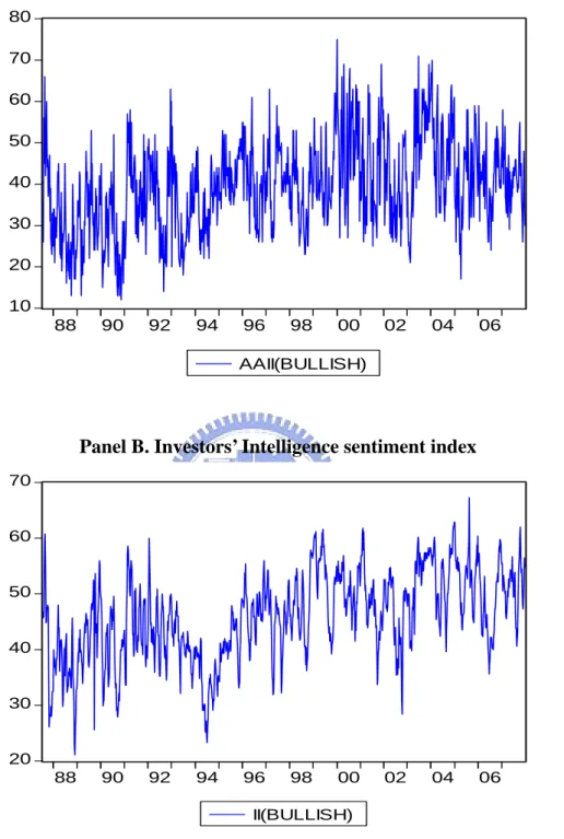
3.1. Direct sentiment measures
There are two indices that directly measure the sentiment of market participants. The first is a
survey conducted by the American Association of Individual Investors (AAII). AAII has
conducted a sentiment survey by polling a random sample of its members each week,
beginning in July 1987. The association asks each participant whether they are bearish, bullish,
or neutral about the stock market in 6 months. Only subscribers to AAII can vote. Since this
sentiment survey is targeted towards individuals, this can be interpreted as an individual
sentiment measure. We use the bullish percentage as a measure of investor sentiment in this
paper.
The second survey is conducted by Investors Intelligence (II). Since 1964, Investors
Intelligence compiles its sentiment data weekly by categorizing approximately 150 market
newsletters. Newsletters are read and marked as bullish, bearish, or neutral starting on Friday
each week. The results are reported on the following Wednesday. We interpret the bullish
percentage compiled by Investors Intelligence as a proxy for institutional sentiment, because a
lot of the writers of those newsletters are past or current market professionals.
Fisher and Statman (2000) use II and AAII index as medium and small investors’
sentiment respectively. They found the relationship between II and AAII sentiment index is
strong and the AAII bullish percentage index is reliable contrary indicators for future S&P
500 returns.
< Figure 1 is inserted about here >
< Table 1 is inserted about here >
their correlation coefficient is 0.513088. AAII and II have strong correlation. But we can see
that AAII fluctuates stronger than II, because AAII represent the small investors’ sentiment
and small investors are influenced by information of market easier than other investors.
3.2. Indirect sentiment measures
Brown et al. (2004) find that many commonly used indirect measures of sentiment are related
to direct surveys of investor sentiment. They examine many financial indicators, which they
categorize into a number of main groups. We use the three categories here, and we choose
some of these indicators as our indirect sentiment measures. In addition, we also add some
market measures in this paper.
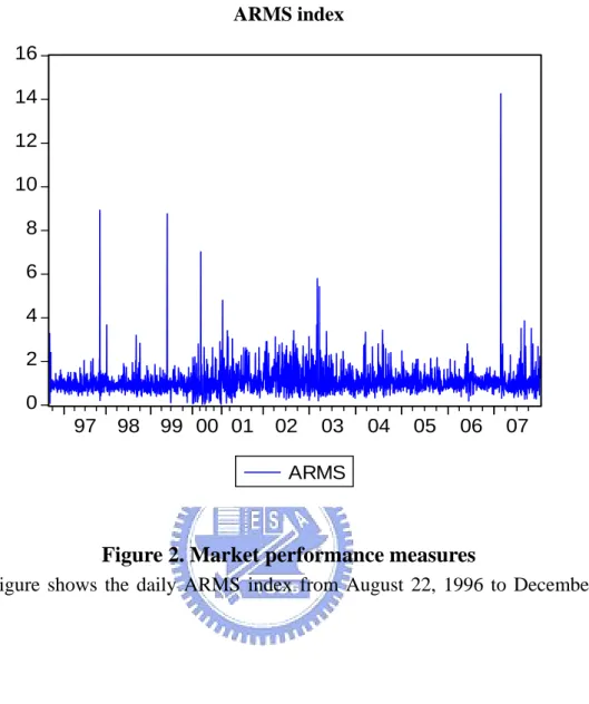
3.2.1. Market performance
The ARMS (or TRIN) index is developed by Richard Arms in 1967 and first introduced by
Barron’s in the same year. One of the first to adopt this indicator in his market analysis was
Richard Russell, the last living Dow Theorist and writer of the Dow Theory Letters. The
ARMS Index is a market breadth and strength indicator, which attempts to analyze the
relationship between the number of advancing and declining issues and the advancing and
declining volume.
The ARMS index is the ratio of the number of advances to declines standardized by their
respective volumes. It is calculated as:
# / /#
# / /#
t t t t
t
t t t t
Adv AdvVol DecVol Dec ARMS
Dec DecVol AdvVol Adv
where #Advt, #Dect,AdvVolt, andDecVolt, respectively, denote the number of advancing issues, the number of declining issues, the trading volume of advancing issues, and the trading
volume of declining issues. An ARMS Index reading of one implies that the market is in
balance, while a reading above one implies more volume is moving into declining stocks
(bearish) and vice versa. When the market is more bearish, the trading volume of declining
issues will rise and the ARMS Index will greater. When the market is more bullish, the
trading volume of advancing issues will rise and the ARMS Index will go down. The ARMS
Index can also be used as an oversold/overbought indicator when smoothed by a simple
moving average – such as using a 10-day or a 21-day moving average. Wang et al. (2006) find
that ARMS has predictive power for future realized volatility. Our ARMS daily data is
obtained form Bloomberg.
< Figure 2 is inserted about here >
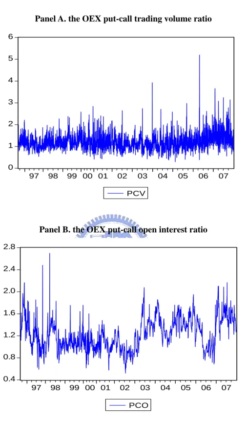
3.2.2. Derivatives variables
The put-call trading volume ratio (PCV) and the put-call open interest ratio (PCO) are also the
measures of market participants’ sentiment. The PCV equals the trading volume of put options
divided by the trading volume of call options. The market participants buy put to hedge their
spot positions, when their sentiment is bearish. The PCV then goes up, because the trading
volume of put options increases in relation to the trading volume of call options, and vice
versa.
We also can calculate the ratio by using the open interest of options instead of trading
volume. The PCO is a good measure of sentiment, because it can reflect the sentiment at the
end of the day or the week. Option open interest is used to proxy for heterogeneous beliefs as
sentiments (e.g. Dennis and Mayhew, 2002). We use the OEX put-call trading volume ratio
and the OEX put-call open interest ration here. The daily data is obtained from Bloomberg.
< Figure 3 is inserted about here >
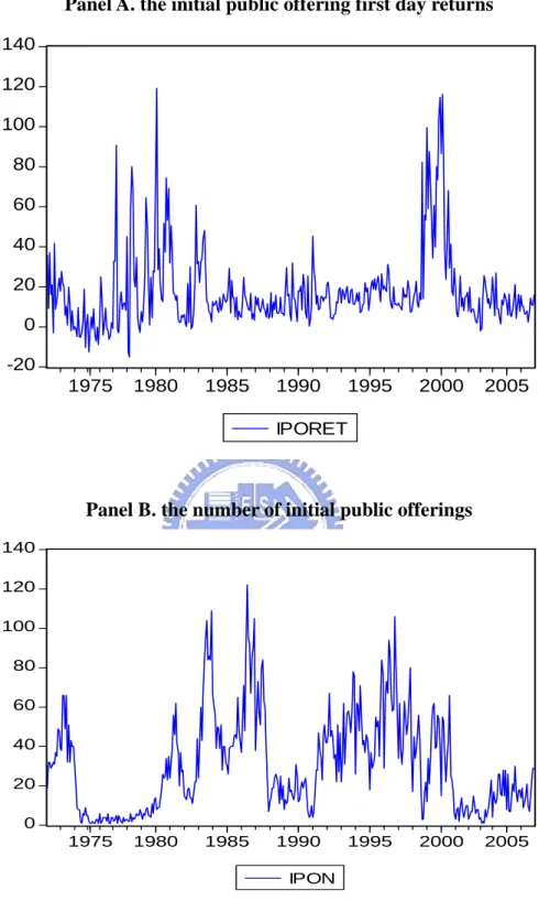
3.2.3. Other sentiment proxies
Many other variables don’t fall neatly within one of the aforementioned categories. IPO
activity is often considered a measure of sentiment because of the information asymmetries
between managers and investors. We include monthly data on initial public offering first day
returns (IPORET) and the number of offerings (IPON) in this paper. The number of initial
public offering and the first day return of initial public offering are both a bullish market
indicator. These IPO monthly data are reported by Ritter (http://bear.cba.ufl.edu/ritter).
< Figure 4 is inserted about here >
3.3. Sample period and stock return proxies
Our daily, weekly, and monthly samples cover the period from August 22, 1996 to December
31, 2007, July 24, 1987 to December 28, 2007, and February 01, 1971 to December 31, 2006,
respectively. Three different market indices which are the DJIA, S&P500, and NASDAQ are
used to characterize the overall performance of the market. The DJIA is a price-weighted
average of 30 large “blue-chip” stocks. Although the limitations in the composition and
construction of the index are well known, yet, it is the most widely followed and reported
stock index. The S&P500 and NASDAQ are both value-weighted indices that reflect the
return of large and small capitalization stocks respectively. The data of DJIA, S&P500, and
NASDAQ are obtained from yahoo finance.
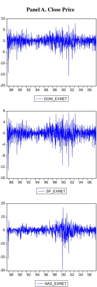
< Figure 6 is inserted about here >
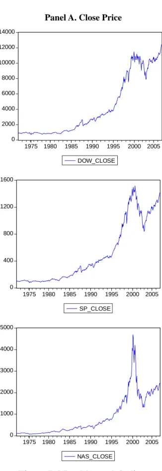
< Figure 7 is inserted about here >
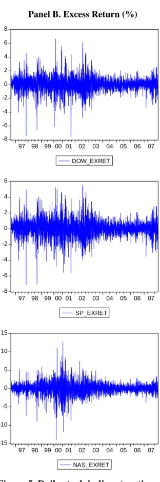
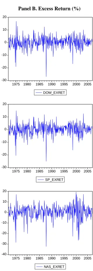
As reported in Panel B of Figure 5, the volatility of excess return of NASDAQ is greater
than DJIA and S&P500, because NASDAQ index is composed of many small high tech
companies where many of their investors are small investor and they tend to be easily
influenced by noise information.
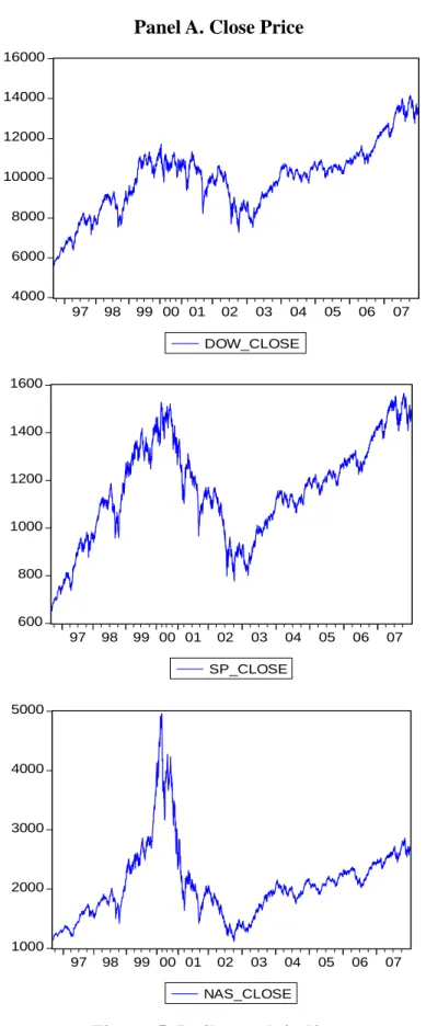
Panel A of Figure 5 shows the daily close prices of DJIA, S&P500, and NASDAQ from
August 22, 1996 to December 31, 2007. As reported in Panel A of Figure 5, we find the close
prices are unusual from March 29, 2000 to April 27, 2000, especially in NASDAQ. During
this period, the close price of NASDAQ drops off substantially from 4958.56 to 3774.03. The
excess returns of stock index are an abnormal negative. It appears commonly in all three
indices and obviously in NASDAQ index. This phenomenon is commonly known as the
bursting of the dot-com bubble.
The average three-month T-Bill yield is used as a proxy for the risk-free rate of interest in
computing the excess returns for each stock index. The daily and weekly three-month T-Bill
yield is obtained from Bloomberg and the monthly three- month T-Bill yield is obtained from
Taiwan Economic Journal (TEJ).
4. Empirical design
4.1. Hypotheses
In De Long et al.’s (DSSW (1990a) hereafter) model, if informed investors have shorter
horizons than noise traders and are concerned with resale prices, arbitrage is limited. Noise
traders’ optimism or pessimism results in transitory divergences between price and
fundamental value. Moreover, the extent sentiment induced takes place contemporaneously
across many assets in the markets, and the additional variability in returns is a systematic risk.
In DSSW, there are four effects of sentiment on returns and volatility shown in Figure 1. We
test two hypotheses that used by Lee et al. (2002). The two hypotheses result from the
interaction of the four effects.
< Figure 9 is inserted about here >
HYPOTHESIS 1 (Direct sentiment effect): The “hold-more” effect dominates the
“price-pressure” effect. When noise traders’ sentiment becomes more bullish, the excess
returns will be higher. If their sentiment becomes more bearish, the excess returns will be
lower.
In DSSW, investor sentiment can influence mean returns directly through two effects,
they are “price-pressure” and “hold-more” effects. The trading of noise traders creates “price
pressure” which results in a purchase (sale) price higher than fundamental value and lowers
expected returns, when the average sentiment of noise traders is bullish (bearish). This is the
“price-pressure” effect.
On the other hand, when noise traders’ sentiment become more bullish (bearish), they will
increase (decrease) demand for the risky assets. This results in a higher (lower) expected
(does not dominate) the “price-pressure” effect, the mean return is higher (lower) while noise
traders’ sentiment becomes more bullish. But when the sentiment of noise traders becomes
more bearish, the net result on mean return is always negative because both effects are
intensifying. Lee, Jiang, and Indro (2002) use the sentiment index which is AAII to examine
these effects, and they find the “hold-more” effect dominates the “price-pressure”.
HYPOTHESIS 2 (Indirect sentiment effect): The “Friedman” effect dominates the
“create-space” effect. A rise in noise traders’ misperceptions about the asset’s risk incurs
lower expected returns.
In DSSW, prices are also affected by changing in the noise traders’ misperceptions about
the asset’s risk. There are two different ways. One of these is the “Friedman” effect. When
many other noise traders are buying (selling), noise traders will buy (sell) most of the risky
asset. Then they will likely suffer a capital loss because of their poor market timing. The more
variable noise traders' misperceptions are, the more damage their poor market timing does to
their returns. The changes in the noise traders’ misperceptions about the risk of the asset incur
lower expected returns.
Another way is the create-space effect. A rise in noise traders’ misperceptions about the
asset’s risk increases price uncertainty and reduces sophisticated investors’ desire to hold
risky assets. Because noise traders’ momentum crowds out risk-averse sophisticated investors,
noise traders benefit more from their trading. Overall, when the “create-space” effect is more
(less) important than the “Friedman” effect, the mean returns are higher (lower).
4.2. The generalized autoregressive conditional heteroscedasticity model
The interaction of four effects results in the impact of noise trading on the risky assets’ price.
noise traders’ sentiment, so they influence mean returns directly. The “Friedman” and
“create-space” effects influence mean returns indirectly through changes in noise traders’
misperceptions of the asset’s risk. Therefore the two effects are related to the magnitude of
the movements in noise traders’ sentiment.
4.2.1. The GJR-GARCH model
Here we use a GARCH-in-mean model which Lee et al. (2002) propose, which includes
lagged shifts in investors’ sentiment in the conditional volatility (variance) equation. It is
different from Lee et al.’s model which includes contemporaneous shifts in investor sentiment
in the mean equation, and it includes lagged shifts in investor sentiment in the mean equation.
0 1 2 3 4 5 1
it ft it t t t it
R −R =α α+ h +α Jan +α Oct +α Dot+ ∆α S− + (1) ε
where R is the return on a market index, it R is the risk-free rate, ft Jan is a dummy t
variable for January effect, Oct is a dummy variable for October effect, t Dot is a dummy variable for dot-com bubble of period, and ∆St−1 is a measure of noise trader risk associated with the shifts in sentiment.1 ∆St−1= ∆SIt−1≡(SIt−1−SIt−2) /SIt−2. Moreover, in equation (1),
~ (0, ) it N hit ε and 2 2 2 0 1 1 2 1 1 3 1 4 5 1 1 2 6 1 1 ( ) ( ) (1 ) it it it t it ft t t t t h I h R S D S D β β ε β ε β β β β − − − − − − − − = + + + + + ∆ + ∆ − (2) where (i)It−1= if1 εit−1< and0 It−1 = if0 εit−1≥ ; and (ii)0 Dt−1 = if0 ∆St−1≤ and 0 Dt−1= if 1
1 0
t
S−
∆ > .
Bollerslev, Chou, and Kroner (1992) suggest that GARCH (1,1) is a parsimonious yet
1
appropriate specification is most applications, therefore we specify only one lag in our
GJR-GARCH model in this paper. Because equity market volatility is found to be higher in
high inflation periods, we include the risk-free interest rate in the variance equation. The
dummy variables, January and October, specify the well-documented seasonal effect in equity
excess returns. Glosten, Jagannathan, and Runkle (1993) specify the dummy variables of the
two seasonal effects and the risk-free interest rate in their GARCH-M model. In addition, we
find the shock of dot-com bubble on stock market caused the close prices to be unusual from
March 29, 2000 to April 27, 2000, especially in NASDAQ. During this period close price of
NASDAQ drop off substantially from 4958.56 to 3774.03 and the excess returns of stock
index are abnormally negative. Then we use a dummy variable to capture the abnormal return
in the period.
We recognize through the dummy variable It−1 that investors in forming their expectations of conditional volatility may perceive positive and negative shocks differently in
Equation (2). In particular, we expect β2 to be positive, because a negative shock is more
likely to cause a larger upward revision of volatility than a positive shock of same magnitude.
This is the leverage effect that is different for negative than for positive shocks. A surprisingly
bad stock market performance causes the debt ratio of the firm to be higher, and investors
perceive the company to be more risky and later revise their expectation of conditional
volatility upward, vice versa. A good stock market performance induces the debt ratio of the
firm to be lower, and investors perceive the company to be less risky and subsequently revise
their expectation of conditional volatility downward.
Many scholars find this asymmetric effect for volatility by empirical researches. For
example, Nelson (1991) finds that news arriving in the market tends to affect volatility in an
asymmetric way, depending on the nature of the news. Glosten, Jagannathan, and Runkle
than for good news.
Moreover, we recognize in Equation (2) through the dummy variables Dt−1 and
1
(1−Dt−) that the magnitude as well as direction of shifts in investor sentiment can have an asymmetric impact on conditional volatility. Individual investors may react differently to the
magnitudes of the shifts in bullish and bearish sentiment in forming expectations of
conditional volatility.
Lee, Jiang, and Indro (2002) find that shifts in sentiment of investor are negatively
correlated with the market volatility. Volatility increases when investors become more bearish
and volatility decreases when they become more bullish,
The coefficients (α5) reflects the net impact of hold-more and price-pressure effects on excess returns in the mean equation. The coefficients (β β5, 6) in the variance equation capture the effect of the magnitude of shifts in sentiment on volatility formation. The net
impact of the Friedman and the create-space effects on excess returns is reflected through the
sign and the significance of the coefficient(α1).
4.2.2. The component GARCH
Engle and Lee (1999) propose the component GARCH model, can separate the conditional
volatility as the permanent and transitory volatility components, and reflect the long-term and
short-term effect. Engle and Lee (1999) also consider the leverage effect and propose the
component GARCH including threshold term. To capture the components of volatility of
noise trader, we estimate a components GARCH model including threshold term.
0+ 1
it ft it
where R is the return on a market index, it R is the risk-free rate, and ft Dot is a dummy variable for dot-com bubble of period.2 Moreover, in equation (3), εit ~ N(0,hit) and
2 2 5 6 1 1 1 7 1 1 8 1 1 2 9 1 1 [ ( ) ] ( ) ( ) ( ) (1 ) it t it t t it t t t t t h q q I h q S D S D β β ε β β β − − − − − − − − − = + + − + − + ∆ + ∆ − (4) 2 2 0 1 1 0 2 1 1 3 1 1 2 4 1 1 ( ) ( ) ( ) ( ) (1 ) t t it it t t t t q q h S D S D β β β β ε β β − − − − − − − = + − + − + ∆ + ∆ − (5)
where (i)It−1= if1 εit−1< and0 It−1 = if0 εit−1≥ ; and (ii)0 Dt−1 = if0 ∆St−1≤ and 0 Dt−1= if 1
1 0
t
S−
∆ > . ∆St−1 is a measure of noise trader risk associated with the shifts in sentiment.
1 1 ( 1 2) / 2
t t t t t
S− SI− SI− SI− SI−
∆ = ∆ ≡ − .
We recognize in Equation (4) and (5) through the dummy variables Dt−1 and (1−Dt−1) that the magnitude as well as direction of shifts in investor sentiment can have an asymmetric
impact on conditional volatility. Individual investors may react differently to the magnitudes
of the shifts in bullish and bearish sentiment in forming expectations of conditional volatility.
The coefficients (β3) and (β4) reflects the long-run effect of noise traders’ sentiment in the variance equation. The coefficients (β8) and (β9) in the variance equation capture the short-run effect of the magnitude of shifts in sentiment on volatility formation. If noise trader
risk affects the volatility is a transitory phenomenon, it will be reflected on the coefficients
(β β8, 9), and we expect the absolute value of the coefficients (β β8, 9) to be greater than (β β3, 4) and the transitory component of sentiment effect is more significant than the permanent component.
2
Because the dummy variables of season effect in the mean equation are not significant and our main purpose is to examine the sentiment effect in the volatility, we only put the dummy of Dot-Com Burble in the mean equation. Although we do not put them in the mean equation, our result does not change.
5. Results
5.1. Summary statistics
< Table 2 is inserted about here >
As reported in Panel A of Table 2, the overall daily returns over the entire sample period are
0.0326% for the DJIA (8.215% annually), 0.0304% (7.661% annually) for the S&P500, and
0.0327% (8.240% annually) for the NASDAQ. The standard deviations of the weekly data are
1.1364 for DJIA, 1.1675 for S&P500, 1.7988 for NASDAQ, and NASDAQ has the largest
standard deviation. The maximum daily return of NASDAQ is 12.6454%, and the minimum
return is -13.9222%. NASDAQ has the largest maximum daily return and lowest minimum
daily return, because NASDAQ index is composed of many small companies.
The excess returns of the three stock indices showed in Panel B are 0.0225% for DJIA,
0.0203% for S&P500, and 0.0226% for NASDAQ and all of excess returns are greater than
zero. It means that there is a positive excess return in the overall stock market in the period
from August 22, 1996 to December 31, 2007. NASDAQ has the highest mean excess return in
the period.
As shown in Panel C, the daily average sentiment indices are 1.0878 for the ARMS,
1.2281 for the put-call open interest ratio, and 1.2106 for the put-call trading volumes ratio,
respectively. The standard deviation of the ARMS, the put-call open interest ratio, and the
put-call trading volume ratio are 0.6166, 0.2796, and 0.3825, respectively. That the means of
the three daily sentiment indices are greater than one means the investors’ sentiments in the
period are more bearish.
ARMS, PCO, and PCV of 0.2456, 0.0038, and 0.0670 respectively, are relatively small. The
means of the three average percentage changes also greater than zero also shows the
investors’ sentiments are bearish in the period.
< Table 3 is inserted about here >
For the weekly data, as reported in Panel A of Table 3, the overall weekly returns over the
entire sample period are 0.1580% for the DJIA (8.216% annually), 0.1469% (7.639%
annually) for the S&P500, and 0.1718% (8.834% annually) for the NASDAQ. The standard
deviations of the daily data are 2.1987 for the DJIA, 2.1355 for the S&P500, 3.1345 for the
NASDAQ. We also see that the NASDAQ has the largest standard deviation and Maximum
weekly return (17.3770%) and the lowest minimum weekly return (-29.1753%).
All of excess returns of stock indices are also greater than zero, so there is positive excess
return in the period from July 22, 1987 to December 31, 2007. The same with the daily data,
NASDAQ has the largest mean excess return in the period of our weekly data.
As shown in Panel C, the AAII has a mean of 39.3827% and a standard deviation of
11.0046, respectively. And the II has a mean of 45.8603% and a standard deviation of 7.8361.
Between the two direct sentiment indices, AAII has the larger standard deviation. Fisher and
Statman (2000) consider AAII represents the small investors’ sentiment and II represents the
medium investors’ sentiment. In average, the medium investors are more bullish than the
small investors. Maybe the small investors are more bullish than medium investors when the
market is bullish and more bearish when the market is bullish, because AAII has the higher
the maximum proportion of bullish and the lower the minimum proportion of bearish.
Panel D shows that over the entire sample period, the average percentage change in AAII
and II of 0.0267 and 0.0029 respectively, are relatively small and the mean of the investor
also larger standard deviation.
< Table 4 is inserted about here >
The period of our monthly data is from February 1, 1971 to December 31, 2006. As
reported in Panel A of Table 4, the overall monthly returns over the entire sample period are
0.6484% for DJIA (7.781% annually), 0.6565% (7.878% annually) for S&P500, and 0.7753%
(9.304% annually) for NASDAQ. The standard deviations of the monthly data are 4.4606 for
DJIA, 4.3905 for S&P500, 6.4486 for NASDAQ, and NASDAQ has the largest standard
deviation. The maximum monthly return of NASDAQ is 19.8653%, and the minimum return
is -31.7919%. NASDAQ has the largest maximum monthly return and lowest minimum
monthly return too. In Panel B, all of excess returns of the three stock indices are also greater
than zero in the period from February 1, 1971 to December 31. 2006 and NASDAQ has the
largest excess return among them.
As shown in Panel C, the monthly average sentiment indices are 17.8290% for the initial
public offering first day return (IPORET) and 30.4171 for the number of offering (IPON). The
number of initial public offering and the first day return of initial public offering are both a
bullish market indicator. More the number of IPO and the first day return of IPO, the market
are more bullish. The standard deviation of the initial public offering first day return and the
number of offering are 17.8290 and 30.4171, respectively. The means of the three daily
sentiment indices are greater than one implies the investors’ sentiments in the period are more
bearish.
In Panel D, the changes in the two sentiment index are greater than zero implies that the
mean of the investor sentiment in the overall market are bullish in the period from February 1,
1971 to December 31. 2006. The means of the changes in the number of IPO and the return of
5.2. Estimated GJR-GARCH results
For each of the three stock indices, we estimate a base model that excludes sentiment as an
explanatory variable in the mean and conditional volatility equations. We estimate
GJR-GARCH in the period from August 22, 1996 to December 31, 2007, July 22, 1987 to
December 31, 2007, and February 1, 1971 to December 31, 2006 for daily, weekly, and
monthly data, respectively. The period of our daily data is approximately ten years and the
period of our weekly data which is approximately twenty years is relatively longer. The
period of our monthly data which is the longest across the three periods is approximately
thirty-five years. The estimated coefficients of the base models for the three stock indices for
daily, weekly, and monthly data are reported in Table 5.
< Table 5 is inserted about here >
First, in the base model, the time-invariant portion of excess returns is not significant; and
the time-varying portion of excess returns in the base model is not significant with conditional
volatility too. The results are not consistent with previous findings of a negative price for
time-varying risk (Glosten, Jagannathan, and Runkle, 1993; De Santis and Gerard, 1997; Lee,
Jiang, and Indro, 2002).
Second, across the three stock indices, not all of the estimated GARCH coefficients in the
base models are significant. We confirm that surprises have an asymmetric effect on
conditional volatility and this result is consistent with our forecast, because most of
coefficients of the asymmetric effect which is β2 are significant and positive except the model of monthly NASDAQ return. Negative shocks cause higher upward revisions in
volatility.
In addition, as Glosten, Jagannathan, and Runkle (1993) find, volatility is generally
coefficients for the risk-free rate are positive and significant for both the DJIA and S&P500.
This result is the same with Lee, Jiang, and Indro (2002). Despite the coefficients for the
risk-free rate of the daily and weekly NASDAQ are not significant and significantly negative,
respectively, it is significant and positive for the monthly NASDAQ.
In our base models, the seasonal effects which are January and October effect are not
significant that only the dummy variables of October effect of monthly DJIA and S&P500 are
significance at 10% level and negative. The season effect is very weak in our data period. The
coefficients of the dummy variables for dot-com bubble in the mean equation are negative and
are significant in the daily models of S&P500 and NASDAQ and weekly models of DJIA and
NASDAQ, especially in NASDAQ (significant at 1% level). But all of dummy variables for
dot-com bubble in the monthly base models are not significant. The impact from the crash of
dot-com bubble to NASDAQ is the largest and the most obvious, because NASDAQ index is
composed of many small high tech companies where many of their investors are small
investor.
To the base model in Table 5, we then add measures of noise trader risk associated with
shifts in sentiment in the mean and volatility equations. The percentage changes in sentiment
for daily, weekly, and, monthly data are utilized in Table 6, 7, and 8, respectively. The major
findings are summarized below.
< Table 6 is inserted about here >
< Table 7 is inserted about here >
< Table 8 is inserted about here >
As shown in Table 6, the time-invariant portion of excess returns and the coefficient of
GARCH in mean equation are not significant. January and October effect is the same as in its
negative only in NASDAQ. The dot-com bubble variable is not significant, except S&P500 of
PCO.
The three sentiment indices which are ARMS, the OEX put-call open interest ratio (PCO),
and the OEX put-call trading volume ratio (PCV) in our daily data are bearish indicators. In
daily model, only the coefficient of lagged shifts in PCO in mean equation for excess returns
of all stock indices are very significant (significance at 1% level) and negative, but PCV and
ARMS are not. We find that PCO can be used to forecast the excess return of a particular
stock index. When the markets are more bearish, PCO goes up. This will affect stock market
in that the excess return of stock market will go down in the future.
In the variance equation of the daily model, after adding the shifts of sentiment, the
phenomenon that volatility is greater when inflation rates are projected to be higher in the
future is no longer clear. In addition, it is the same with base model that surprises have an
asymmetric effect on conditional volatility. This is the leverage effect that is different for
negative than for positive shocks and the magnitude of the change in market volatility is
greater for bad news than for good news.
For the models of ARMS, we find bullish shifts in sentiment in the current period result in
statistically significant downward revisions in the volatility of future returns, and the
coefficient of bearish shifts in ARMS in variance equation are very small. For PCO and PCV,
bearish shifts in sentiment in the current period lead to upward revisions in volatility of future
returns. Bullish shifts in PCO and PCV in the current period also lead to upward revisions, but
it is less significance (only NASDAQ p-value is less than 5%). We find the three daily
sentiment indices are good indicators to forecast the volatility of excess return of stock index.
As reported in Table 7, we use two direct sentiment indices AAII and II as the bullish
variable of dot-com bubble for each indices and sentiment are significant and great negative
other than DJIA for AAII.
First for AAII, in mean equation, the time-invariant portion and the time-invariant portion
of excess returns of DJIA and NASDAQ are not significant. But the time-invariant portion of
excess return of S&P500 is significant and negative (-0.908) and its coefficient of GARCH in
mean equation is significant and positive (0.159). We find AAII in the current period can be
used to forecast the excess return of S&P500 in the future, because the coefficient of the shift
of AAII is significant at 5% level and positive (0.771). When AAII rises, it will affect stock
market in that the excess return of stock market will go up in the future. In variance equation,
we don’t find the surprises having an asymmetric effect on conditional volatility and it is
surprising that the coefficients of the risk-free rate are negative. We find that bullish shifts in
AAII sentiment index in the current period result in statistically significant downward
revisions in the volatility of future returns of DJIA and S&P500, and the coefficient of bearish
shifts in AAII in the variance equation are not significant.
Second in the models of II, in the mean equation, each time-invariant portions and
coefficient of GARCH-in-mean are not significant. In the mean equation for DJIA and
S&P500, a shift in sentiment has a significant positive impact on excess return and the
coefficients of DJIA and S&P500 are -1.576 and -1.559, respectively. It means the II is a
good contrary indicator for the excess returns of DJIA and S&P500, especially for S&P500.
In the variance equation, there is the leverage effect that is different for negative than for
positive shocks, but II in the current period can’t affect the volatility in the future.
As shown in Table 8, we use IPON and IPORET as bullish sentiment index in our
monthly data. In Table 8, we don’t find IPORET in the current period can affect the excess
return in the future and each of coefficients of October effect is significant. Although IPORET
coefficient is very small. So we can say with confidence that IPORET has poor forecasting
power.
In addition, we find that when IPON rises, the excess returns of S&P500 and NASDAQ
will go up in the future. However, IPON also has forecast power for the volatility of
NASDAQ, bullish shifts in sentiment in the current period result in statistically significant
downward revisions in the volatility of future returns.
Overall, we find that investor sentiment is an important factor in explaining equity excess
returns and changes in conditional volatility. PCO can be used to forecast the excess returns
of all stock indices. As PCO goes up, the excess returns will go down. AAII can be used to
forecast the return S&P500 and II can be used to DJIA and S&P500. There is positive
correlation between excess returns and shifts of AAII, but there is negative correlation
between excess returns and II. When the bullish percentage of II rises up, the excess return
will go down. We confirm II is a contrary indicator for excess returns of large capitalization
stocks, because II represents the newsletters’ sentiment and they are medium investors. Their
opinion will affect other investor especially with the small investors and AAII represents the
small investors’ sentiment. Although there is great positive correlation (0.513) between AAII
and II in Table 1, their results are very different. We consider that AAII might be close to
noise traders’ sentiment. We also find that there is a positive relationship between change in
IPON in the current period and excess return of S&P500 or NASDAQ.
Our results show that shifts in sentiment have an asymmetric impact on conditional
volatility. As the magnitude of shifts in bullish sentiment increases, there is a downward
(upward) revision in the volatility of future returns. First, PCO and PCV can be used to
estimate the effect of change of bearish sentiment to excess return of volatility, and ARMS
can be used to estimate the effect of change of bullish sentiment. Second, when change of
return of DJIA and S&P500 which are large stock will go down in the future. But the effect of
the change of bearish sentiment within AAII is not as clear. IPON also has the same effect,
but there is some difference in that it is for volatility of NASDAQ.
However, only AAII used as a sentiment indicator to estimate the excess return of
S&P500 fits in with our empirical hypothesis which is the noise trader model of De Long et al
(1990a), so we use this result to explain the economical reasoning. In the mean equation, a
shift in sentiment has a statistically significant positive impact in excess return. The
hold-more effect tends to dominate the price-pressure effect and leads to an increase in excess
returns when noise traders are more bullish in their sentiments. In particular, when sentiment
becomes more bullish, optimism induces noise traders to hold more of the risky assets than
fundamentals would indicate, this secures the compensation for bearing the increase in risk
associated with sentiment. Nevertheless, the higher risk premium due to increased demand is
partially offset by the unfavorable price at which noise traders transact.
If sentiment becomes more bearish, there is a reduction in excess returns. Noise traders
choose to hold less of the risky assets when they are more pessimistic, and consequently, are
unable to capture the risk premium related to sentiment. Moreover, there is a negative price
impact caused by sentiment-induced sale of securities.
In the volatility equation, we also find that bullish shifts in sentiment in the current period
result in significant downward revisions in the volatility of future excess returns. And bearish
shifts in sentiment in the current period lead to upward revisions in volatility of future excess
returns. As the magnitude of shifts in bullish (bearish) sentiment increases, there is a
downward (upward) revision in the volatility of future excess returns resulting in lower
(higher) future excess returns.
where they end up buying high and selling low. The Friedman effect implies that asset prices
tend to be negatively affected when noise traders’ misperceptions are more severe. But the
extent that asset prices are adversely influenced by the Friedman effect depends on the space
which noise trading creates. The lower excess return associated with volatility revisions due
to bullish sentiment shifts indicates that the positive effect on price of the space created by
sentiment-induced noise trading is not large enough to offset the negative effect on price of
poor market timing. In contrast, there is a higher excess return associated with volatility
revisions due to bearish sentiment shifts. In this case, the positive effect on price associated
with noise trader created space is sufficient to offset the negative effect on price associated
with poorly timed sales of securities triggered by bearish shifts in sentiment.
5.3. Estimated Component GARCH results
Here we find some sentiment indices can affect the volatility of excess return of stock index,
so we try to use the component GARCH to find whether the noise trader risk is only a
transitory phenomenon. The estimated component GARCH results for daily, weekly, and,
monthly data are utilized in Table 9, 10, and 11, respectively. The major findings are
summarized below.
< Table 9 is inserted about here >
As reported in Table 9, the coefficients of dummy variable of dot-com bubble are
significant for NASDAQ in the daily data, and most of the time-invariant portion of excess
returns is positive and significant. First, in the transitory component, all the coefficients of
threshold term (β6) are positive and most of them are significant, hence the leverage effect still exist. We also find that the magnitude of the percentage change in sentiment has a
shifts in sentiment in the current period result in statistically significant downward revisions
in the volatility of future returns, but bearish are not obvious except S&P500 for PCO (1.102)
and PCV (8.541) and NASDAQ for PCV (-0.011). Although -0.011 is positive and significant,
the value is very small.
Second, we also find some results in the permanent component. For ARMS, we also find
the same result that Bullish shifts in sentiment in the current period result in statistically
significant downward revisions in the volatility of future returns and the shifting of bearish is
not statistically significant.
In addition, we find that the absolute value of the coefficient of sentiment shift in the
transitory component is greater than in the permanent, but it seems not very clear for
NASDAQ.
< Table 10 is inserted about here >
For weekly data, shown in Table 10, the coefficient of the magnitude of the change in the
AAII sentiment is not significant. But it is not the same with II sentiment. The coefficients of
(β6) are 88.170, 95.093, and 130.1932 for DJIA, S&P500, and NASDAQ, respectively which are positive and statistically significant. For NASDAQ, both that bullish shifts in sentiment in
the current period result in statistically significant downward revisions in the volatility of
future returns and bearish shifts in sentiment in the current period result in significant upward
revisions in the volatility of future returns. Especially, we find that the short-run effect of
noise traders’ sentiment is greater than the long-run effect.
< Table 11 is inserted about here >
But in our monthly data, the coefficient of the magnitude of the change in sentiment does
not have a significant impact on the conditional volatility, no matter in the permanent or
6. Conclusion
The model of De Long, Shleifer, Summers, and Waldmann (1990a) predicts that the direction
and magnitude of changes in noise trader sentiment are relevant in asset pricing. It is
mispecified and at best incomplete because the empirical tests focused on the impact of
sentiment either on the mean or variance in asset excess returns alone.Lee, Jiang, and Indro
(2002) use a GARCH framework to jointly test the four behavioral effects delineated in the
noise trader model of De Long, Shleifer, Summers, and Waldmann (1990a). Their
specification allows us to explicitly test the impact of noise trader risk on both the formation
of conditional volatility and expected return as suggested by De Long, Shleifer, Summers, and
Waldmann (1990a). They only use a direct measure of investor sentiment compiled by
Investors’ Intelligence to proxy noise trader risk. We also use a GJR-GARCH framework to
test the four effects in the noise trader model, but we use more sentiment indices to proxy this
kind of risk and include lagged shifts in investor sentiment in the mean equation. There are
seven sentiment indices which are use in this paper. For example there are ARMS, OEX
put-call trading volume ratio (PCV), OEX put-call open interest ratio (PCO), AAII, II, the
number of initial public offering (IPON), and the initial public offering first day returns
(IPORET). We try to find whether the sentiment can affect the excess return and volatility.
First, we find that PCO can be used to forecast the excess return of stock index. When the
market are more bearish that PCO goes up, it will affect stock market that the excess return of
stock market will go down in the future. AAII and IPON have the same effect on S&P500 and
NASDAQ, respectively. However, II is a good contrary indicator for excess returns of DJIA
and S&P500.
Second, we find that the three daily sentiment indices (ARMS, PCO, and PCV) are good
good indicators to forecast the volatility of excess return of large and small capitalization
stock, respectively. We find that shifts in sentiment are negatively correlated with the market
volatility; that is, as volatility increases (decreases) investors become more bearish (bullish).
The significance of sentiment on conditional volatility implies that conventional measures of
temporal variation in risk omit an important factor.Moreover, Lee, Shleifer, and Thaler (1991)
find that closed-end fund discounts which proxy for investor sentiments have the highest
correlation with the smallest stocks. But we examine among the three indices, sentiment does
not have the most profound impact on NASDAQ. This is not consistent with the finding of
Lee, Shleifer, and Thaler (1991) and Lee Jiang, and Indro (2002). Sentiment and noise trading
not only affect the volatility of the small capitalization stocks, but also large capitalization
stocks. In this paper, we use NASDAQ index as the proxy of small capitalization stocks. But
NASDAQ index is composed of many small high technology company, we can not exclude
the conclusion that traders’ sentiments affect the stocks of high technology industry, not small
capitalization stock.
In addition, although only one of our models which use AAII as sentiment on excess
return of S&P500 fits for the four effects of De Long et al. (1990a) and the inclusion of
sentiment changes the negative relation between the equity excess return and conditional
volatility documented in prior studies (Nelson, 1991; Glosten et al., 1993; Lee et al., 2002),
we find that lower excess returns are associated with a decrease in conditional volatility
resulting from larger bullish shifts in sentiment. These results are consistent with the market
reaction to noise trading as suggested by Friedman and create-space effects of De Long et al.
(1990a). In this model, there is a positive relation between shifts in sentiment (AAII) and
excess returns (S&P500) which indicate that the increase in risk premium associated with the
hold-more effect is relatively more important than the negative impact of the price-pressure