有效能源的拓樸控制於行動無線隨意網路之研究

國

立

交

通

大

學

電機學院與資訊學院 資訊學程

碩

士

論

文

有效能源的拓樸控制於行動無線隨意網路之研究

Energy-efficient topology control for mobile wireless ad hoc networks

研 究 生：黃莉婷

指導教授：簡榮宏 教授

有效能源的拓樸控制於行動無線隨意網路之研究

Energy-efficient topology control for mobile wireless ad hoc networks

研 究 生：黃莉婷 Student：Li-Ting Huang

指導教授：簡榮宏 Advisor：Rong-Hong Jan

國 立 交 通 大 學

電機學院與資訊學院 資訊學程

碩 士 論 文

Submitted to Degree Program of Electrical Engineering and Computer Science College of Electrical Engineering and Computer Science

National Chiao Tung University in Partial Fulfillment of the Requirements

for the Degree of Master of Science

in

Computer Science January 2006

Hsinchu, Taiwan, Republic of China

有效能源的拓樸控制於行動無線隨意網路之研究

學生：黃莉婷

指導教授：簡榮宏

國立交通大學電機學院與資訊學院 資訊學程﹙研究所﹚碩士班

摘

要

對於無線隨意網路中的移動裝置而言, 節約電源是延展裝置壽命

的關鍵因素, 無線隨意網路中主要的傳輸工作是尋找路由以及傳遞資

料, 我們探討網路拓樸型態對於傳輸工作的影響。本篇論文針對不同種

類的傳輸需求, 探討如何選擇當時最省電的拓樸型態, 藉由動態改變

網路拓樸, 使得整體的電力應用達到最大效益。就省電的拓樸型態而言,

r-鄰區圖形( r-Neighborhood Graph, 簡稱

)是目前能動態控制網路

拓樸的方法

, 在本篇論文中, 我們分析

結構的特性

, 並且探討

DSDV 路由協定結合

控制拓樸型態, 對於電源消耗所帶來的助益。

Energy-efficient topology control for mobile

wireless ad hoc networks

Student：Li-Ting Huang

Advisors：Dr. Rong-Hong Jen

Degree Program of Electrical Engineering Computer Science

National Chiao Tung University

ABSTRACT

The power saving problem is a key issue in mobile ad hoc networks.

Topology control is a common method for power saving. This thesis

focuses on how to select a topology for the ad hoc network in which nodes

consume the least power in data transmission. The r-Neighborhood Graph,

denoted as

, is structure has special properties for topology control. In

this thesis, the properties of

structure are analyzed and then the

combination of the destination-sequenced distance-vector

routing protocol

and

in controlling topology, which brings the benefit in power

誌

謝

我要感謝我的指導老師簡榮宏教授, 這兩年來不斷給我研究上的指

導, 即使超過時間也仍然給我幫助, 除了課業上的指導, 也不忘關心

我和我的家人, 讓我在忙碌和壓力之外, 還感受到一些溫馨的鼓勵。

再來要感謝博士班學長鄭安凱, 學長一直指點我研究的方法, 在我做

實驗感到茫然時, 能即時點醒我正確的方向。另外要感謝我的人生伴

侶鍾久林, 謝謝他的包容以及在生活上他帶給我的一切支援。還有許

多關心我幫助我的家人好友們, 我也一併致上衷心的感謝。

目

錄

中文提要

...

i

英文提要

...

ii

誌謝

... iii

目錄

... iv

圖目錄

...

v

Chapter 1

Introduction ...

1

Chapter 2

Background and Motivation ...

4

Chapter 3

Fundamental of NGr ...

9

Chapter 3.1 Basic theory ...

9

Chapter 3.2 Measuring formulae ...

9

Chapter 3.3 The r-Neighborhood Graph ... 10

Chapter 3.4 GG, RNG and their relationships respect to

11

Chapter 3.5 Construction algorithm ... 13

Chapter 3.6 Sparseness of

... 13

Chapter 4

Topology Control in Wireless Ad Hoc Networks . 15

Chapter 4.1 Route selection ... 15

Chapter 4.2 Static wireless ad hoc network ... 15

Chapter 4.3 Power-cost of routing ... 16

Chapter 4.4 Turning the parameter r ... 17

Chapter 4.5 Mobile wireless ad hoc network ... 18

Chapter 5

Beaconing Mechanism ... 20

Chapter 5.1 Mechanism ... 20

Chapter 5.2 Frame format ... 21

Chapter 6

Simulations and Analysis ... 23

Chapter 6.1 Simulation environment and parameters ... 23

Chapter 6.2 Methodology ... 25

Chapter 6.3 Overview of the components ... 28

Chapter 6.4 Simulation results ... 29

Chapter 7

Conclusion ... 43

List of figures

Fig 3-1 The r-neighborhood region of node u and v ……….. 10

Fig 3-2a The GG circle of u and v ………... 11

Fig 3-2b The RNG lune of u and v ……….. 11

Fig 3-3 The upper boundary of power stretch factor for

when

n=100 and α= 2 ………..

12

Fig 3-4 The upper boundary of maximum node degree for

... 13

Fig 3-5a The sparseness of

with r = 0.0 ………... 14

Fig 3-5b The sparseness of

with r = 0.5 ………... 14

Fig 3-5c The sparseness of

with r = 1.0 ………... 14

Fig 4-1 The overhead of DSDV partial rerouting in a mobile

network ………..

19

Fig 4-2 The ratio of control packets in a mobile network ………….. 19

Fig 6-1 Two-ray ground reflection model ……….. 25

Fig 6-2 Average of transmission radius of nodes on UDG and

. 30

Fig 6-3 Average of transmission power for broadcast-based traffic .. 31

Fig 6-4 Average of hop count of 10 connections on 100 nodes …… 32

Fig 6-5 Average of end-to-end delay of 10 connections on 100

nodes ……….

33

Fig 6-6a Average of degree of 100 nodes tuned by

……… 34

Fig 6-6b The maximum node degree in theory and in the experiment. 35

Fig 6-7 Average of transmission radius of 100 nodes ……….. 35

Fig 6-8 Average of broadcast power of 100 nodes ……… 36

Fig 6-9 Transmission power of all (including successful and

unsuccessful) packets ………

38

Fig 6-11 Average of transmission power for successful packets ……. 39

Fig 6-12 The best r for each level of mobility as total nodes is 50 …. 40

Fig 6-13 The best r for each level of mobility as total nodes is 100 … 41

Fig 6-14 The best r for each level of mobility as total nodes is 200 … 41

Fig 6-15 The comparison of consumed power on

, GG and

RNG for 50 nodes ……….

42

Fig 6-16 The comparison of consumed power of

, GG and

RNG for 100 nodes ………...

42

Fig 6-17 The comparison of consumed power of

, GG and

1. Introduction

A wireless ad hoc network is a group of wireless communication devices which set up a possibly temporary network for the communication needs. Hosts on such network are able to move arbitrarily due to the lacking of restrictions imposed by wires. The topology defined by such a network can be very arbitrary, as there are no constraints on where hosts can be located with respect to each other. All hosts are mobile and are connected dynamically in an arbitrary appearance. In wireless ad hoc networks, all communications are carried out through wireless links in a distributed fashion without the aid of centralized administration. Hence a wireless ad hoc network can be quickly constructed without additional equipments. It is very suitable for emergency services, sensor dust, dada acquisition in inhospitable terrain, and conferencing in which mobile users gather outside their normal office environments, etc.

Due to the wireless capacity and limited transmission range of each device, a long-distance communication must go through multi hops in wireless ad hoc networks. However, since there is no fixed infrastructure resident, each host has to act as a router and packer forwarder. Routing protocol is performed on every host and consumes the resources at each host. The feasibility of transmission at nodes is heavily depends upon the routing protocol. A good routing protocol should minimize the computing load and the traffic overhead in wireless ad hoc networks.

The problem of routing is essentially finding the shortest-path (basing on various metric). A number of routing protocols derived from link-state or distance-vector routing algorithm. In link-state approach, each node gathers information about the state of links that have been established between the other nodes. In distance-vector approach, each node collects routing information and maintains a routing table containing the cost

and the next hop to a destination. Such protocols are classified as proactive or reactive depending on when and how the routes are discovered. Proactive protocols also called table driven protocols because nodes keep track of routes for all destinations in ad hoc networks, they store route information even before it is needed. Take some well-known protocols for examples, DSDV [1], WRP [2], FSR [3] and CGSR [4] belong to proactive protocols. Reactive protocols also called on-demand protocols, in which routing information is acquired only when it is actually needed. For examples, AODV [5], DSR [6], TORA [7] and ABR [8] belong to reactive protocols.

There are many varieties derived from the well-known protocols base on every of scenario. For most protocols, the algorithm itself can be applied for arbitrary topology. By simplifying a network topology might enhance the efficiency or reduce cost on that algorithm. We concern with the usefulness in saving energy for each node. A set of nodes and their connecting relationships in network can be seen as a graph. One pair of node has an edge if they can directly communicate to each other. To reduce the power-cost of performing routing protocol, a subgraph is needed; and to guarantee the delivery on the converting graph, a connected graph is needed. We introduce the sparse planar graph. The sparse planar containing a spanning tree satisfies these requirements. Topology control is done by routing procedure. Routing procedure extracts a graph from the network as a topology and then applies routing along the edges on the graph, thus transmission path is formed under such topology. In which topologies decide the cost of all transmissions need, and controlling the topology is important in routing stage. Existing localizable structures counting for planar are GG [9], RNG [10], Del [11] and

NG_r [12], etc. Each structure keeps special feature for certain purposes. Among them,

NG_r is the only one by which routing procedure can dynamically convert network’s topology so far. In this thesis, we illustrate the basic property of NG_r and discuss how

to tune the topology to adapt to different transmission circumstances. Our experiment and analysis verify the theory and provide suggestions benefiting with energy-efficient for mobility scenario.

The rest of this thesis is organized as follows. Chapter 2 discusses the background and motivations. Chapter 3 illustrates the fundamental of NG_r. Chapter 4 discusses the topology control in mobile ad hoc networks and chapter 5 demonstrates a beaconing mechanism in Mac layer. A series of simulations and analysis are shown in chapter 6. And in chapter 7, we give the conclusion at the end.

2. Background and Motivation

Number of qualitative characters of routing scheme is introduced in [13] and [14]. In this thesis we concern with power efficiency, scalability and distributed operation. We take account of routing procedure from these aspects of view and explain why NG_r

structure is suitable for controlling topology. They are described as below.

Power efficiency

In many kinds of ad hoc network, the mobile nodes operate on battery power. However, despite devices are getting more powerful in computing but battery technology have not yet reach advances. Device equipping with battery must not always keep full energy without recharge. Mobile nodes distributed in ad hoc networks might exhaust their energy due to their transmission activities. Nodes consume power when they transmit data to desire recipients, but in most situations, nodes contribute their energy and as intermediate nodes to forward data for other nodes. Moreover, numerous routing protocols discover routes by flooding. When flooding, nodes participating in the network must broadcast control messages as possible as they can. Broadcasting might consume lots of their energy. For a mobile node with limited energy, power-saving mechanisms must be applied to extend its battery life.

In a broadcast-based traffic network, lessening the number of broadcasting in network is feasible to save energy. It is rational that a node has not to forward messages to all of its neighbors as long as messages can be guaranteed delivering to their recipients. To reduce the number of relaying, a spare network is good for this. Network itself is not necessary spare, but can form a spare topology by meant of certain manners. Planar is an example of sparer topology than the original one by eliminating crossing links. All

planar structures we mentioned here, GG, RNG, Del and NG_r, are suitable for this demand. Routing scheme can thus reconstruct the topology as a subset of the original network and perform routing on that topology.

In a unicast-based traffic network, there are two aspects of improvement in energy conservation on each node. One is lessen the power on transmitting, and the other is finding optimal routes to minimize total of power consumed. The former can be easily realized in wireless device, and the later is carried out by letting power consumed of each transmission be metric on link and launching routing algorithm to find the most economical path. Routing algorithm running on a planar should be careful because not all of planar algorithms take account of both eliminating links and guaranteeing the optimum of routes. Del, GG and NG_r have the feature in keeping all necessary links to compose the path as efficient as the original topology, while others might not.

Although all planar structures we mentioned can satisfy at least one of these two situations for energy conservation, only one of them can satisfy both and dynamically control the topology to adapt to these two situations. That is NG_r. It is important to examine its effects on battery life and to find a suitable topology so that it does not compromise communication performance. By constructing and adjusting NG_r, routing protocol can take the best efficiency in power saving.

Scalability

Routing algorithms should perform well for mobile wireless ad hoc networks with arbitrary number of nodes. Sensor networks is one kind of mobile wireless ad hoc networks, there might have hundreds or thousands of nodes in them. It is not ensure that the size of a wireless network can grow, routing scheme has to establish contacts for all nodes, no matter what the number of node is. A scalable solution is one that performs

well in large networks.

Flooding-based route discovery is widely assumed in existing routing protocol of mobile wireless ad hoc networks. In such protocol, control messages might broadcast through the whole network until finding their targets. Network-wide flooding enables the discovery of optimal routes from sources to destinations. However, too many nodes participate in the network would result in much more control messages to be disseminated. The increased number of control messages places additional load on the available bandwidth, which is usually already a constraining factor for communication between wireless nodes. Transmission of control messages may cause undesirable load on each node as well as on the available network bandwidth. Heavy transmission in a large scale network would seriously hurt the limited resources on that network. Node mobility introduces other kind of scalability problem in wireless ad hoc networks. Since the routes change as mobile nodes move, control messages have to be sent around the network to represent current connectivity information. The task of reestablish of routes is due to the lost links or the newly discovered links. These control messages are likely to be broadcasted more often if the level of node mobility is higher.

The two key factors relating to scalability are the size of network and the mobility of nodes. Number of nodes take a directly effect on flooding. We can’t reduce the number of nodes participating in the network but the number of control messages. There are ways to suppress redundant messages relay, for instances, restricting the control messages to transfer within limit opportunity (limit region, limit period, etc.), or directly restricting the number a control message can broadcast.

Routing on a simplifying topology takes an advance on restraining the redundancy of control messages. The overhead of flooding is depended on the degree of node, and the degree usually increases as the size of a network grows. If node degree of network is

bounded by a topology, routing burden will be greatly reduced. RNG and NG_r can bound the maximum node degree of a network under some conditions. Topology control algorithm itself must be localized to adapt to large scale and high mobility environments. An algorithm is localized if it makes its decision using only the information of node within constant hops, and the additional cost of detecting global network is not required. Number of node varies at any time, and topology controlling should be adapted to the various circumstances. NG_r can archive this goal. In the following section, we will see that in some cases the maximum degree can be bounded in a constant by NG_r no matter how large the network is. By limiting the degree, routing protocol can perform well in a large scale network. However, keeping a topology with less links may sacrifice some potential routes consuming less energy in a denser topology. Therefore, a tradeoff is between the less node degree and more link selections, and adjusting NG_r is exactly for this goal.

Distributed operation

Number of topology constructing dependent on geographic information, it is not hard for nodes to acquire geographic information by modem techniques. The distance between neighboring nodes can be estimated on the basis of incoming signal strengths or time delays in direct communications. Nodes sense the signal strength from their surroundings to aware neighbors. Relative coordinates of neighboring nodes can be obtained by exchanging such information between nodes. Alternatively, the location of nodes may be available by communicating with GPS (Global Positioning system), if nodes are equipped with a small low power GPS receiver. Nodes without GPS receiver can also obtain their positions by location algorithm. To use such algorithm, there must be some known position nodes resident in the network, coordinating with ranging

technology, relative or absolute position can be computed for unknown position nodes. There are centralized system and distributed system for positioning. The centralized system has a server to process location queries, while distributed system in which nodes calculate positions by themselves. Centralized system is less feasible because additional traffic is inevitable during the querying time. A localizable topology construction algorithm, such as NG_r, is naturally suitable for distributed system.

Position based scheme becomes practical because of the advance of hardware and location algorithm. Nodes have geographical information about other nodes can help making decision on transmitting, either as on topology constructing. Topology control algorithm usually collects all geographical information from nodes to maintain a global view of network. In constructing NG_r, only local view of nodes is required. If one network desires to form into NG_r, every node just needs to care about their one-hop neighbors. Hence no centralized server is required and no additional traffic is wasted, routing procedure spends control messages only for its routing activities.

3. Fundamental of NG_r

3.1 Basic theory

On a two-dimension plane_{R with a set V of n wireless nodes, a widely accepted} 2 basic graph-theoretical model for network is the unit disk graph (UDG). In such graph, any two nodes u and v are joined by an edge if and only if the Euclidean distance between their coordinates, denoted as||uv , is at most R, where R is the transmission || radius, which is equal among all nodes in the network. The least power required to transmit immediately between u and v is modeled as||uv||α

, where α is typically taken on a value between 2 and 4, depending on the attenuation strength of the communication environment [15].

3.2 Measuring formulae

To measure the power efficiency of a topology, a well-formed measure, named Power stretch factor [16] is introduced below.

Let π( , )u v =v v v v_{0 1}... _{h−1 h} be a unicast path connecting nodes u and v, where v₀ = u

and v_h = . The total transmission power consumed by path ( , )v π u v is defined as

1 1 ( ( , )) h || _{i i}|| i p π u v v v₋ = =

∑

π be the least-energy path connecting nodes u and v in graph G(V).

Given a subgraph G’(V) of G(V), the power stretch factor of G’(V) with respect to G(V) is defined as * '( ) ' _, * ( ) ( ( , )) ( ( )) max ( ( , )) G V G _{u v V} G V p u v G V p u v π π ∈ = ρ

G(V) is defined as

max( ( )) max_{u V} G V( )( )

d G V d u

∈

= , where d_{G V( )}( )u is the degree of node u in graph G(V).

3.3 The r-Neighborhood Graph

The r-Neighborhood Graph [12], denoted asNG (V)_r , with parameter r, 0 ≤ r ≤ 1, is proposed by Jeng and Jan. NG (V)_r is a geometric structure on two-dimension plane, which can always result in connected planar topology with symmetric edges. We introduce the structure as below.

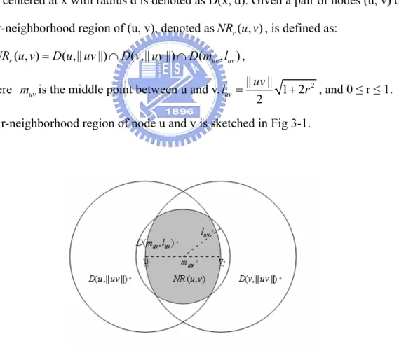
The r-neighborhood region is defined at the first. Let x be a point on_{R , the open} 2 disk centered at x with radius d is denoted as D(x, d). Given a pair of nodes (u, v) on_{R ,} 2 the r-neighborhood region of (u, v), denoted asNR u v_r( , ), is defined as:

( , ) ( ,|| ||) ( ,|| ||) ( , )

r uv uv

NR u v =D u uv ∩D v uv ∩D m l ,

Where m is the middle point between u and v,_uv || || _{1 2} 2 2

uv

uv

l = + r , and 0 ≤ r ≤ 1.

The r-neighborhood region of node u and v is sketched in Fig 3-1.

Fig 3-1: The r-neighborhood region of node u and v.

on_{R , the r-neighborhood graph of V, denoted as}2 _{NG (V)}

r , has an edge uv if and only if ||uv|| ≤ R and NR u v_r( , ) contains no node w є V, where 0 ≤ r ≤ 1.

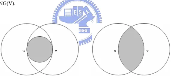
3.4 GG, RNG and their relationships respect toNG_r

The constrained Gabriel Graph [9], denoted as GG(V) and the constrained Relative Neighborhood Graph[10], denoted as RNG(V), are the two extreme cases of NG (V)_r . GG and RNG have similar algorithm forming planar graph but different qualified regions, the regions are sketched in Fig 3-2(a),(b), respectively. For any set V of nodes on _{R , there has the relationship} 2 _{RNG(V) NG (V) GG(V)}

r

⊆ ⊆ , for all 0 ≤ r ≤ 1.

NG (V)_r is equivalent to GG(V) with r = 0 and is equivalent to RNG(V) with r = 1, by increasing the parameter r, the scale of NG (V)r can be tuned from GG(V) toward RNG(V).

Fig 3-2a: The GG circle of u and v. Fig 3-2b: The RNG lune of u and v.

For a n nodes topology, GG(V) has the optimal power stretch factor 1, which is much better than the unbounded power stretch factor n-1 of RNG(V) . However, the maximum node degree of GG(V) could be as large as n-1, while the maximum node degree of RNG(V) is bounded to 6 if there is no node in V having two or more neighbors at exactly the same distance. Therefore, GG(V) and RNG(V) are mutually

complementary with respect to the power stretch factor and the maximum node degree. There are no prefect structure satisfying these two criterions, either of GG(V) and RNG(V) has advantage to supply the other one, NG (V)r is designed to fill this gap.

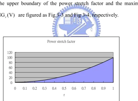
From the theorem, power stretch factor and the maximum node degree of NG_r can be partially bounded into constants. For the power stretch factor, if the underplayed UDG(V) was connected, NG (V)_r is partially bounded by the formula:

( ( )) 1 ( 2)

r

NG UDG V ≤ +r n− α

ρ , for all 0 ≤ r ≤ 1 and α ≥ 2. …Eq 3-1

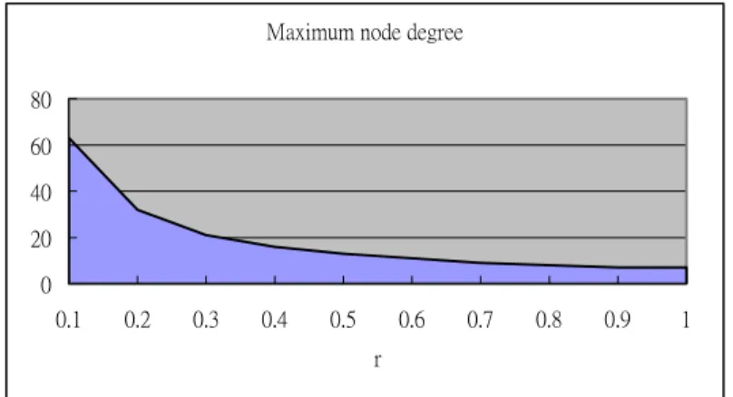
For the maximum node degree, NG (V)r is partially bounded by the formula:

_max( ( )) ₁ sin ( / 2) r d NG V r π −   ≤  

 , for all 0 ≤ r ≤ 1. …Eq 3-2

The upper boundary of the power stretch factor and the maximum node degree for

NG (V)r are figured as Fig 3-3 and Fig 3-4, respectively.

Power stretch factor

0 20 40 60 80 100 120 0 0.1 0.2 0.3 0.4 0.5 0.6 0.7 0.8 0.9 1 r

Maximum node degree 0 20 40 60 80 0.1 0.2 0.3 0.4 0.5 0.6 0.7 0.8 0.9 1 r

Fig 3-4: The upper boundary of maximum node degree forNG (V)r .

3.5 Construction algorithm

NG (V)_r can be locally constructed by nodes. Under some detecting scheme, all nodes know about their immediate neighbors, if u and v can reach one another, they must know the r-neighborhood region between them. Each node u starts the constructing from the full list of its neighbors N, and remove non-NG (V)r links as follows:

3.6 Sparseness of NG_r

Form the definition of NG (V)r in page 10, the parameter r decides how large the for all v є N do

for all w є N do

if w == v or w == u then continue

else if ||uw|| < ||uv|| and ||vw|| < ||uv|| and ||m w|| < uv luv eliminate edge (u, v)

break end if end for end for

r-neighborhood region constrains and how strict the edge uv exists. The eliminating of edges directly changes the degree of node u, by tuning the parameter r, nodes can change the sparseness of NG (V)r . Figs 3-5(a),(b),(c) demonstrate the sparseness of

NG (V)_r with r = 0.0, r = 0.5 and r = 1.0, respectively.

(a) r = 0.0 (b) r = 0.5 (c) r = 1.0 Fig 3-5: The sparseness of NG (V)r .

4. Topology Control in Wireless Ad Hoc Networks

4.1 Route selection

From the view of route selection, it is surely that UDG(V) has the best power efficiency because there are complete links providing the appraising on finding routes. Any of subgraph of UDG(V) might sacrifice some potential routes consuming less energy, hence the power efficiency of a subgraph must not better than UDG(V). The formula of power stretch factor present the maximum ratio of transmission power consumed of all paths between UDG(V) and its subgraph. For any subgraph, a smaller factor is preferred because its effect is near the original graph, factor 1 is the best result because it has the same effect as UDG(V). For the measuring formula toNG (V)r , the power stretch factor of NG (V)_r is constant when r is 0 or some sufficiently small value. The factor of NG (V) is 1, this implies that ₀ NG (V) has identical energy ₀ efficiency as UDG(V). In Fig 3-3, we saw that the upper boundary of power stretch factor forNG (V)r strictly increases as r increases. The factor of topology bounded by a lower value surely results better efficiency, and vice verse. Eq 3-2 explains that

0

NG (V) has the best power efficiency of all NG (V)r with r ranged from 0 to 1, and the efficiency is worse as r increase, finally, NG (V)₁ has the worst efficiency among all.

4.2 Static wireless ad hoc network

Routing protocols commonly have two opportunities to find routes, the first one is route discovery phase, in this phase a node devises a way to collect routing information; the second one is route repair phase, in this phase, broken routes cause a node to reestablish the contacts between pairs. Nodes with fixed positions form a static network.

In a static network, the performing of routing is only once and rerouting is rarely needed. Hence a static network should concern with the power-cost of transmitting data not the routing. Initial topology is rather important because it decides the power-cost of data transmission later consumed. Eq 3-2 shows that r = 0 leads to the minimal power consumed in NG (V)r among all r. Base on the principle of power stretch factor, a static network should control its topology to be NG (V)_r with the parameter r set to 0.

0

NG (V) must have all necessary links to compose the best routes consuming less power for all source-destination pairs. Routing algorithm can view the topology of network as NG (V) and perform routing on the topology, as long as run time of ₀ routing algorithm is long enough, nodes can eventually obtain the best routes for all pairs. After that, all data transmissions enjoy the result of routing. It is clearly that communication in the network is the most efficient under such routes if nodes keep their topology unchanged.

4.3 Power-cost of routing

Numerous distributed and localized routing protocols are based on flooding [17]. In wireless ad hoc networks, a node with a lower node degree can avoid excessive network flows pass through it. For a flooding-based routing algorithm, the cost of routing is heavily dependent on the node degree, which is the multiplication factor of control packets grown. Consider the maximum node degree in a topology, nodes in any set of

NG (V)r has much lesser node degree than UDG(V), even so, the level of node degree can further be tuned by parameter r in NG (V)_r . Recall the Fig 3-5, we have seen the sparseness of NG (V)r with different r, the sparseness is also restricted by Eq 3-3. The maximum node degree of NG (V) is not bounded because it could be as large as n-1. ₀ In Fig 3-4, we saw that the upper boundary of maximum node degree forNG (V)r

strictly decreases as r increases. The degree bounded by a lower value surely results lower degree, and vice verse. NG (V)_r with higher r has lower maximum node degree than NG (V)r with lower r, NG (V)1 unquestionably has the least node degree among all. Hence, a flooding-based routing protocol should control the topology of a network to be NG (V)r with the parameter r set to 1 in routing phase.

4.4 Tuning the parameter r

From the preceding logic, NG (V) is energy-efficient for data transmission and ₀ 1

NG (V) is energy-efficient for routing, but in realistic networks, there are not always data or control packets. Each of these two topologies could not absolutely be applied throughout the time. Especially in a mobile network, the node mobility results the change of topology and possibly induces rerouting. This would change the cost of paths and vary the total of power efficiency in networks. The best solution is adjusting the network topology to obtain the advantage of NG (V) or ₀ NG (V)₁ . According to the transmission requirements, a tradeoff is between the power stretch factor and the maximum node degree. Other scale between them is needed in some circumstances, and by tuning the parameter r a network can obtain desired property. The threshold of r is estimated by how much the type of traffic near to data-based or how much far from flooding-based. The level can be quantified as the ratio of data packets and control packets through the network. If the quantity is small, the network traffic will trend to data-based, and a smaller r is preferred; if the quantity is large, the network traffic will trend to flooding-based, and a larger r is preferred. Routing procedure can dynamically tune the r forming various topologies to adapt to different circumstances, depend on the type of traffic. If the parameter r is tuned correctly, the network will obtain better benefit in power efficiency.

4.5 Mobile wireless ad hoc network

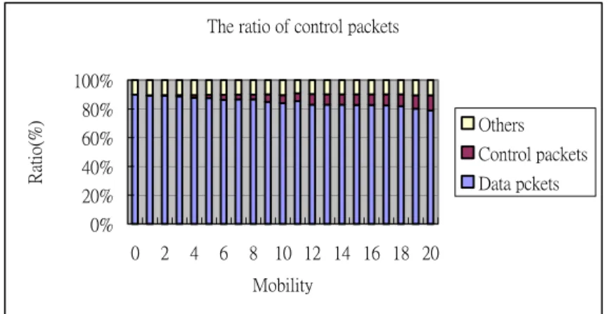
In wireless ad hoc networks, there are often mobile nodes roaming around the network. Node mobility usually disturbs the normal traffic and hurt the performance of data transmission. The maintenance of routes is complex and less efficient, and a mobile network has to spend more routing cost to keep the network works. Node mobility usually causes rerouting due to the two reasons: the first reason is changes of cost on path, and the second reason is broken of links. Repair of routes could be a partially routing. The expense of partially routing is not large as the global routing, but greatly takes effects on network. Level of node mobility, such as moving speed, pausing time, or number of moving node in network, examines the feasibility of routing algorithm. If node mobility is high, expense of rerouting will be much. The occurrence of rerouting depends on the level of mobility, and one rerouting might lead to much more control packets generated. We observe the overhead of the advertisement for routes’ changes on DSDV in a mobile network, as shown in Fig 4-1, the number of control packets multiply grows as the number of rerouting increase, which is a typical character of flooding. It is certainly that if there is no data transmission in network, NG (V)₁ will be preferred because its sparseness could minimize the overhead of flooding. If there is data transmission, one should consider other topology more suitable thanNG (V)₁ . In Fig 4-2, we observe the ratio of routing transmission in a mobile network, in which routing procedure view the topology as NG (V)r with r = 0.5, the figure shows that as the level of mobility gradually increase, loading of control packets in network increases, in other word, loading of data packets decreases. The appearance of control packets is relatively less but its affect is great because the broadcast power is much large than unicast power. The network with the lowest mobility should control its topology to be

0

NG (V) and the network with the highest mobility should control its topology to be 1

NG (V). The topology can be adjusted by r to be one between NG (V) and ₀ NG (V)₁ , we expect that the best r is located depends on node mobility, as the level of mobility is small, the value r should be small because the effect of power stretch factor is still workable; as the level of mobility is high, the value r should be high, but if node mobility reach one threshold, that is, the effect of flooding is great, the highest r will be always preferred. 0 20 40 60 80 100 120 140 160 1 2 3 4 5 6 7 8 9 10 11 12 13 Number of rerouting N umber o f br oadcas ting

Fig 4-1: The overhead of DSDV partial rerouting in a mobile network.

The ratio of control packets

0% 20% 40% 60% 80% 100% 0 2 4 6 8 10 12 14 16 18 20 Mobility Ra tio(%) Others Control packets Data pckets

5. Beaconing Mechanism

In this section we introduce a beaconing mechanism in Mac layer. The constructing of NG (V)_r requires nodes to know about their one-hop neighbors and the distances between them. We design a beaconing mechanism for nodes to aware their neighbors. Assume that each node knows about the position for itself, all nodes in network asynchronously inform their geographical data to others. If one node does not know about its position, it may provide the transmitting parameters to neighbors for the estimation of destinations. By creating a neighbor list and cooperating with Mac layer, routing procedure can locally construct NG (V)_r for network.

5.1 Mechanism

Each node creates a neighbor list which saving all of its one-hop neighbor and the distances between them. One node should deal with the node mobility in networks hence a higher frequency in informing is required. Every node periodically broadcasts its position data or transmitting information as a beacon without the need of acknowledge at a period of one second. On such frequency, nodes do not worry about the miss of the beaconing frame from others because the next beacon will be come soon. To avoid the synchronization of neighbors’ beacons, nodes have to jitter each beacon’s transmission by 50 % of the interval between beacons. Every node receiving the beacon from a neighbor checks its neighbor list and updates the destination data for the beacon owner. One neighbor is though as fail or gone out of range if a node continuously misses three beacons from that neighbor, and the old neighbor is deleted from its list. Physical layer should control its transmitting power as the normal power of antenna for broadcasting beacons, thus that mobile nodes do not lose any possibly neighbor. The

control of broadcasting power for beaconing frame is irrelevant respect to the network layer. The controlling of power in network layer is for saving energy while the controlling of power in Mac layer is for finding neighbors.

5.2 Frame format

To minimize the overhead of the beaconing in network, nodes broadcast their positions without the need of acknowledge. The fewest data a node should know are the existence of neighbors and their distances between the node and neighbors, hence a simply frame is required. The maximum size of payload in Mac frame body is 2304 bytes, and only 10 bytes are scoped for this beaconing. The size is so small that the beaconing frame does not need to be fragmented. For a broadcast objective, a broadcast address (0xffffffffffff) is recorded in the Address1 field, and the frame header labels the usage of beaconing. Position data or transmitting parameters in frame body is encapsulated as following format:

4 1 1 4

Node Identity Sequence

Number

Data Identity

Data

The first field records the source node’s identity (such as an IP), the second field records the sequence number for distinguishing different beacons, the third field is data identity and the forth field records the data related to the data identity. Three types of data are supported in data field. Each node can provide position or transmitting parameters for ranging the destination. The data field records position of the node if data identity is 0, the first two bytes is x coordination and the last two bytes is the y

coordination, each of them is formed in a floating number. The data field records transmitting power of the node if data identity is 1, receiving nodes compare the transmitting power and the sensed power to estimate the distance through a ranging algorithm. The data field records transmitting time of the node if data identity is 2, receiving nodes calculate the time delay and estimate the distance by dividing the speed of light if these two nodes are time synchronization.

If a node has known about its position, it could broadcast the position directly. If a node has not known about its position, it could send out the transmitting parameter on packets. Receiving nodes estimate the distance by range algorithm. One node has better to provide position information, if not, the second choose can be applied. This beaconing mechanism is an easy way to obtain the distances from neighbors, and the advertising information is sufficient for nodes to construct NG (V)_r .

6. Simulation and Analysis

Several of simulation based studies are introduced in [18] [19] [20]. In this chapter, we launch a serial of experiments. The goals are described as follow:

(1) To compare the efficiency of UDG(V) and NG (V)r ; (2) To discover new feature of NG (V)_r ;

(3) To verify the effect of power stretch factor and node degree; (4) To find the best r for mobile networks.

6.1 Simulation environment and parameters

Simulator

We evaluate energy consumption on NG (V)r by using a network simulator, ns2 package. It uses OTcl as a command to build up a network environment and work the traffic and movement pattern in the network. Ns2’s kernel provides complete protocol stack for wireless networks, we can modify some of then to realize our communication model.

Mac protocol

The IEEE 802.11 distributed coordination function (DCF) Mac protocol has been implemented in ns2 kernel. It use RTS/CTS/DATA/ACK pattern for all unicast packets and simply sends out DATA for all broadcast packets. The implementation uses both physical and virtual carrier sense. Several of important parameters must be tuned up here, in 802.11 Mac layer, RTSThreshold is set to 180 to avoid unnecessary control packets, (there are, RTS and CTS). ShortRetryLimit and LongRetryLimit are both

enlarged to extend the number to transmit packet. The former reduce packets’ collision, the latter enhance the delivery rate of packets.

Ratio propagation model

Through all of our simulations, Two-ray ground reflection model is chosen as radio propagation model. This model reflects the relation among signal power on transmitter, signal strength the receiver can sense and propagating distance between them. Detailed formula is described in the official document of ns2 [20], we figure the curve as Fig 6-1 by assuming that the received signal power is fixed on 1.559e-11 watt. To achieve enough power a receiver can sense, transmitting power must be large to overcome the weakness caused by distance. Fig 6-1 illustrate that transmitting signal power is direct proportion to distance, that is, the nodes are closer, required power is lesser. Normal transmission range in ns2 is 250.010651…., but distances between neighbor nodes on

NG_r are usually much less than this value, this shows that the nodes on NG_r are very suitable for applying power control.

Energy model

To measure consumed power in ns2, radio propagation model should combine with energy model. In OTcl script, each node is given with an initial value as level of energy at the beginning of simulation, say 0.1 joules, this value is known as InitialEnergy. It also has a given energy used for every packet it transmits or it receives, these are called TxPower and RxPower. Another value, IdlePower, represents the power consumed during idle time, we only interest in InitialEnergy and TxPower. InitialEnergy is constant on each node, and the energy carried by a node is continuously decreased according to its channel status (transmitting, receiving, or idling). Base on radio

propagation model, transmission power is function of transmission radius as mention in the preceding section, so TxPower should vary when packet being sent.

0 50 100 150 200 250 0 0.005 0.01 0.015 0.02 0.025 0.03 0.035 0.04 0.045 0.05 Distance(meter) T rans m itt ed s ignal pow er (w at t)

Two-ray ground reflection model

Fig 6-1: Two-ray ground reflection model.

6.2 Methodology

Geographical scheme

Our experiment supposes that all nodes have the ability to aware the positions of their neighbors. Geographical information is important because it is useful in locally constructing NG_r topology and controlling power on packet transmitting. Researches have proven that power control can improve the utilization of channel, and routing applying topology construction in our experiment can further show that energy is more efficiency on transmitting packets.

Power Control

Power control is designed by assuming that every node can choose a power level to transmit a packet. This innovation not only increases the utilization of channel but also reduces the energy required. Traditional method is sensing the power level received from a node and estimating a value as transmission power to transmit packet on that level next time. The shortest distance between nodes can be regarded as transmission radius. If the transmission distance is known by others, the transmission power will be easily estimated by radio propagation model. The estimated value should be enlarged to protect from errors caused by node’s movement or signal interference. This ensures the receiver to catch the packet. Power control can also be applied on broadcasting. If one node desire to broadcast packets to its neighbors, the distance of the farthest neighbor can be used for calculating the broadcast power.

Mobility model

To approach reality in life for ad hoc networks, nodes’ movement is poured into network. Surveys of mobility model are introduced in [21]. Among them, Random Walk Mobility Model is used to behave node mobility. It was developed to act like irregular movement and nodes’ movements are independent of each other. . In Random Walk mobility Model, each node starts its journey from a random location, and randomly chooses a direction and speed to travel, then moves toward that direction for a predefine time (or distance), once the destination is reached, another journey is restart instantly. These activities are repeated till the end of simulation time. A mobility model usually examines the efficiency of a routing protocol. It is difficult to discovery a good route to a moving node, or to repair a route from moving nodes. We produce nodes’ movement

here to observe the energy consumed in the duration of route’s unstable time.

NG_r

NG_r is a structure counting for planar. A planar is a graph that there are no links across to each other in such a graph. A sparse topology is formed by eliminating these crossed links. NG_r is common model of GG and RNG, the parameter r is able to be tuned form 0.0 to 1.0 such that the topology is translated from GG toward RNG. GG might be good on some situations but bad on other situations, either as RNG. By changing the parameter r can adjust the topology for network to obtain the property on GG or RNG, even on any scale between them. In our experiments, routing protocol is constructed on the top of NGrto evaluate the benefit in energy consumption. Packets are transmitted via the edges on NG_r, receiving nodes drop packets if they does not have the NGr edge to the sender. Especially in flooding step, a packet is transmitted in a ‘broadcast power’, irrelevant nodes might involve into this transmission. The principle ensures that packets are always transported on NGr edges in network.

DSDV

Typical routing algorithms are introduced in [22]. Our goal is discussing the effect on topology construction attached to routing scheme, DSDV [1] built in ns2 is suitable for this. DSDV is based on the idea of the classical Bellman-Ford routing algorithm with certain improvements. Every node maintains a routing table and periodically broadcasts the routing table to its immediate neighbors. A node also broadcasts its routing table if a significant change has occurred from the last update sent. On the receiving node, the up-to-date route information might correct its routing table and trigger another broadcast to its neighbors. All of activities go on till all routing tables are stable. DSDV

require every node to learn about every other node in the network, this kind of routing is based on full information. The optimal rout can be elected in such scheme if run time of DSDV is long enough. Our optimal route is the route elected from all possible routes that the smallest energy is spent for two nodes, so we predict energy consumption for each packet and use the value to instead of hop count as metric of DSDV.

CBR

One test scenario is traffic model. We use CBR (continuous bit-rate) to generate traffic on nodes. CBR is built in ns2 and laid on the application layer. It works with UDP agent and periodically transmits packets between nodes. CBR is started at a specific time, the source-destination pairs are spread randomly over the network, source node continuously issue packets in a bit-rate. By changing the number of traffic sources, we can get scenarios with different traffic load.

6.3 Overview of the components

To illustrate protocols used in our experiment more clearly, we make some comments for improvement from the view of network architecture. Our design is implemented on multiple layers, they are described as below:

Application layer CBR

Network layer DSDV on NGr

Mac layer 802.11Mac and Beaconing mechanism

6.4 Simulation results

Common parameters

There are common parameters in the following experiments. In our simulations, nodes are uniformly distributed in a 1000 m * 1000m field. Number of nodes is dependent on each experiment. Each node is given 100 joules as InitEnergy. If there is data to transmit, CBR sources would continuously issue data packets at a period of 1 second, each data packet carry with 1000 bytes as payload. Finally, all simulations are performed within 50 seconds.

Experiment 1: node density and energy consumption

The number of nodes is range from 25 to 250. Number of nodes can be regard as density and referred by the following formula:

Density n( ) n

wxh

= ,

where n is the number of nodes; w and h are width and height of the field respectively. We compute the average transmission radius for every pair of nodes and launch a simulation. Transmission radius is defined as the shortest distance between two nodes they have an adjacent edge on topology and can directly communicate to each other. This information is important to the following experiment. At this fist experiment, we concern with control packet, so no data is transmitted. 25 nodes are designed to periodically broadcast its routing table every 10 second. UDG and NG_r are applied in all densities, and the parameter r in NGr is fixed on 0.5. We settle the energy

consumption and average them for 25 nodes at the end of simulation time.

Average of transmission radius is shown in Fig 6-2. Transmission radius of nodes on

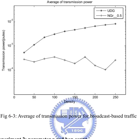
NGr is down as density increases but on UDG is almost at the same level for all densities. Fig 6-3 figures the average of transmission power for the 25 nodes. In Fig 6-3, transmission power on NGr is always lower than on UDG in all densities.

Nodes in dense networks have smaller transmission radius, this is because nodes in dense network are usually close to each other and transmission radius among them are relatively small. UDG has not the function to adjust topology so transmission radius keeps on a level. We observe Fig 6-3, the curve of UDG rises due to large consumed power and its following collisions. Collisions cause more cost of retransmission.

Comparing the energy consumption with NGr and UDG, energy consumption on

NG_r has fluctuation and is much smaller than on UDG. Power control is applied both on UDG and NGr, but we can see that the efficiency on NGr is more conspicuous than on UDG. 0 50 100 150 200 250 40 60 80 100 120 140 160 180 Density T ran sm is si on r adi us (m et er )

Average of transmission radius

UDG

NGr₀.5

Fig 6-2: Average of transmission radius of nodes on UDG and NGr. 0 50 100 150 200 250 10-4 10-3 10-2 Density T ran sm is si on po w er (jo ul es )

Average of transmission power

UDG NGr__0.5

Fig 6-3: Average of transmission power for broadcast-based traffic.

Experiment 2: parameter r and hop count

100 nodes are in the field and traffic is generated by 10 CBR connections. The parameter r of NG_r is ranged from 0.0 to 1.0. We calculate the average of hop count and end-to-end delay for the 10 CBR source-destination pairs.

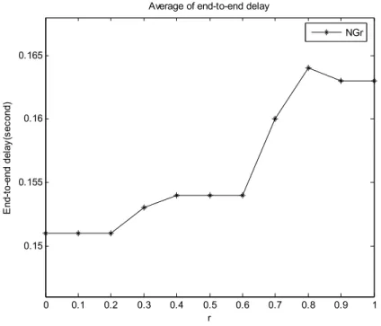
As shown in Fig 6-4, nodes on NG_r with lower r has shorter hop count, and higher r cause longer hop count. A path with longer hop count usually implies larger end-to-end delay of transmission nodes. We can see the result in Fig 6-5, end-to-end delay of transmission nodes increases as r increases.

It is not difficult to understand why higher r leads to longer hop count. We explain this from the two extreme cases of NGr: GG and RNG. By the definition, RNG is a

subgraph of GG. RNG drops some edges in GG to form an exacter planar. Due to the reason, routing protocol on NG_r might find longer hop to compose a path. Packet spends more steps to reach its destination usually hurts the latency on nodes. We conclude that if the latency is important to a network, the lower r should be chosen.

0 0.1 0.2 0.3 0.4 0.5 0.6 0.7 0.8 0.9 1 18 18.2 18.4 18.6 18.8 19 19.2 19.4 r H op c oun t

Average of hop count

NGr

0 0.1 0.2 0.3 0.4 0.5 0.6 0.7 0.8 0.9 1 0.15 0.155 0.16 0.165 r E nd- to-end de lay (s ec ond)

Average of end-to-end delay

NGr

Fig 6-5: Average of end-to-end delay of 10 connections on 100 nodes.

Experiment 3: parameter r and flooding

100 nodes are in the field, and traffic is generated by 10 CBR connections. The parameter r in NG_r is ranged from 0.0 to 1.0. For each r, we calculate the average of degree, transmission radius and broadcast power on nodes. Broadcast power is calculated by assuming that each broadcast carries with 1,000,000 bytes in a packet. Degree of a node is the number of NGr edge indicated to that node due to the bidirectional transmission of nodes. And broadcast power on node is defined as the energy consumed for transmitting packet to its farthest neighbor that has an NGr edge to that node.

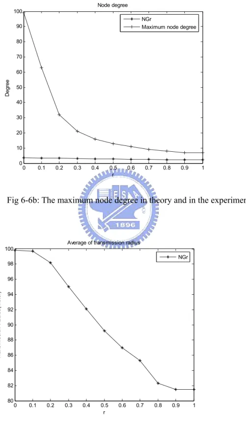
Fig 6-6(a),(b) reveals that the node degree can be adjust by parameter r in NGr. The degree decreases as r increases, this result confirms with the theory of maximum node degree in Eq 3-3. Nodes with lesser degree form a spare network, and spare network can

protect redundancy and congestion from storming traffic generated. Transmission radius can be adjusted by parameter r, too. As shown in Fig 6-7, transmission radius is shorten by the higher r, this implies that nodes can spend smaller power to communicate to each other. Another measurement in Fig 6-8 is the broadcast power. Broadcast is also down as r is up, the tendency is similar as Fig 6-7.

Many of routing protocol discover routes by flooding packets, but too much control packets would burden the whole network and interfere with normal data traffic. Routing on NG_r has the property of reducing unnecessary flooding by reason of node degree. Lesser degree causes fewer nodes to participate in the transference of control packets, this efficiently suppress redundant packet relayed. Besides, broadcast power is consumed on every time to broadcast packet, a smaller broadcast power signifies that the cost of energy would greatly reduce on flooding. By observing Fig 6-6 and Fig 6-8, we conclude that if a flooding based routing protocol runs in a network, NGr with higher r applied into the protocol brings the better efficiency in saving energy.

0 0.1 0.2 0.3 0.4 0.5 0.6 0.7 0.8 0.9 1 2.2 2.4 2.6 2.8 3 3.2 3.4 r D egr ee

Average of node degree

NGr

Fig 6-6a: Average of degree of 100 nodes tuned by NGr. 0 0.1 0.2 0.3 0.4 0.5 0.6 0.7 0.8 0.9 1 0 10 20 30 40 50 60 70 80 90 100 r De gr ee Node degree NGr

Maximum node degree

Fig 6-6b: The maximum node degree in theory and in the experiment.

0 0.1 0.2 0.3 0.4 0.5 0.6 0.7 0.8 0.9 1 80 82 84 86 88 90 92 94 96 98 100 r T ran sm is si on R adi us (m et er )

Average of transmission radius

NGr

Fig 6-7: Average of transmission radius of 100 nodes.

0 0.1 0.2 0.3 0.4 0.5 0.6 0.7 0.8 0.9 1 0.006 0.007 0.008 0.009 0.01 0.011 0.012 0.013 0.014 0.015 0.016 r T rans m is si on P ow er (jou le s)

Average of broadcast power

NGr

Fig 6-8: Average of broadcast power of 100 nodes.

Experiment 4: parameter r and data transmission

100 nodes are in the field and traffic is generated by 10 CBR connections. We measure the total of consumed energy and collision rate for each r, and observe the relationship between them.

As shown in Fig 6-9, it looks like the minimal power consumed is located on 0.5, and transmission power on range 0.0 to 0.3 is slightly larger than range 0.4 to 0.6, range after 0.6 is rapidly up until 1.0. We also observe the collision rate in Fig 6-10, the collision rate rise just at range 0.4 to 0.6.

At an ideal, collision-free network model, nodes on NGr with lowest r must have better path to delivery packets. By the theorem, selection of path decrease as r increases. The tendency act on transmission would result in the energy consumption increases as r

increases. Curve in Fig 6-9 is not smooth because of range 0.4 to 0.6. In practice, collisions normally occur in medium access schemes. Fig 6-10 shows that lots of collisions appear in the middle range, too much collisions cause dropping packets. The decrease of energy in reality is result from the fewer number of transmissions. We explain how the collision concentrates at the middle. From the theorem, lower r leads to more degrees on node (refer to Fig 6-6 in experiment 3), if degree of every node increases, their transmission path would close to each other. We expect that the probability of collision greatly enlarge at the lower r. On other hand, lower r also leads to smaller consumed power, and smaller power might influence lesser nodes in its transmission radius. So the probability of collision is canceled out by the smaller power, and the appearance of most collision shift to the middle of r range not at the low. We should consider about the delivery rate and normalize the energy consumption by calculating the average of transmission power of packet has successively delivered. This result is shown in Fig 6-11. We can see that consumed power certainly increases as r increases, and this curve verifies power stretch factor in Eq 3-1 and is more closely to theorem.

0 0.1 0.2 0.3 0.4 0.5 0.6 0.7 0.8 0.9 1 0.298 0.299 0.3 0.301 0.302 0.303 0.304 0.305 0.306 0.307 0.308 r T rans m is si on P ow er (jou le s) Transmission Power NGr

Fig 6-9: Transmission power of all (including successful and unsuccessful) packets.

0 0.1 0.2 0.3 0.4 0.5 0.6 0.7 0.8 0.9 1 2 2.2 2.4 2.6 2.8 3 3.2 3.4 3.6 3.8 4 r C ollis io n R at e( % ) Collision Rate NGr

0 0.1 0.2 0.3 0.4 0.5 0.6 0.7 0.8 0.9 1 9.2 9.25 9.3 9.35 9.4x 10 -4 r T ran sm is si on P ow er (joul es ) Transmission Power NGr

Fig 6-11: Average of transmission power for successful packets.

Experiment 5: energy consumption and node’s movement

50,100 and 200 nodes are respectively in the field. 10% of nodes create CBR connections and continuously issue data. DSDV routing protocol is modified to check neighbors’ link statuses every second. If any change is found, the up-to-date route is flooded in the network. There are x nodes move within the field in random walk model. The speed of movement is 2m/s. We estimate energy consumption and find out the best r for each x. The best r is defined as the value r* leads to the minimal energy consumption in NGr among the range 0.0 to 1.0.

Fig 6-12, Fig 6-13 and Fig 6-14 figure the curve for 50, 100 and 200 nodes respectively, r* starts at the below or middle position of r range if there is no any node moves, as the level of mobility increases, r* increases toward higher position of r range. Node movement would cause routes’ change, and lead to partial rerouting. DSDV

periodically check neighbors’ link status, two cases might happen, the first is that new neighbor move into its transmission radius, and the second is that an old neighbor moves out of its transmission radius. According to the DSDV protocol, route’s change would trigger a partial flooding, and receiving nodes stop their broadcasting if routing table is stable. Experiment 4 shows that in a data-based network, the parameter r is good on lower value; and the experiment 3 shows that in a flooding-based network, the parameter r is good on higher value. As the number of moving nodes increase, the ratio of control packets increases, the best r is therefore located at the higher position, so r* is up as mobility increases. The result for 50 nodes increases more quickly than the other two, the reason is that 50 nodes in the field is already sparse, the effect of power stretch factor is relatively small, hence a little flooding traffic cause r* to rise. The comparisons of consumed power on NG_r*, GG and RNG are shown in Fig 6-15, Fig 6-16 and Fig 6-17, respectively. Power efficiency of NGr_* is always equal or better than the other two. This result verifies our inference in character 4.

0 2 4 6 8 10 12 14 16 0 0.2 0.4 0.6 0.8 1

Number of moving node

r*

50 nodes

Fig 6-12: The best r for each level of mobility as total nodes is 50. 0 2 4 6 8 10 12 14 16 0 0.2 0.4 0.6 0.8 1

Number of moving node

r*

100 nodes

NGr

Fig 6-13: The best r for each level of mobility as total nodes is 100.

0 2 4 6 8 10 12 14 16 0 0.2 0.4 0.6 0.8 1

Number of moving node

r*

200 nodes

NGr

50 nodes 0 0.1 0.2 0.3 0.4 0.5 0 2 4 6 8 10 12 14

Number of moving node

C ons um ed powe r NGr* GG RNG

Fig 6-15: The comparison of consumed power on NG_r*, GG and RNG for 50 nodes.

100 nodes 0 0.1 0.2 0.3 0.4 0 2 4 6 8 10 12 14

Number of moving node

C ons um ed powe r NGr* GG RNG

Fig 6-16: The comparison of consumed power of NG_r*, GG and RNG for 100 nodes.

200 nodes 0 0.1 0.2 0.3 0.4 0 2 4 6 8 10 12 14

Number of moving node

C ons um ed powe r NGr* GG RNG

7. Conclusion

The energy-efficient topology control can enhance the efficiency or minimize the power-cost of communications. By adjusting a topology for a network, the network can achieve the desired property in power-saving. NGr structure counting for planar is applied for this objective. NG_r can be locally and adaptively constructed into sparse topology for a network, routing procedure works on such topology finding the optimal routes. By changing the parameter r of NG_r, the network can obtain the advantage of GG, RNG, or any scale topology between them. Our simulations verify the result from the theory, and discuss the difference between the reality and the theory. New feature is also found in these experiments. Finally, the best r which leads to the minimal consumed power is examined for node mobility. The variation of r explains the benefit of controlling NGr in which a mobile wireless ad hoc network can get the most efficiency in power saving.

References:

1. C.E. Perkins and P. Bhagwat, “Highly dynamic destination-sequenced distance-vector routing (DSDV) for mobile computers”, Proceedings of ACM

SIGCOMM’94, pp. 234-244, August 1994.

2. S. Murthy and J.J. Carcia-Luna-Aceves, “An efficient routing protocol for wireless networks”, ACM Mobile Networks and Applications Journal, Special issue on

Routing in Mobile Communication Networks, pp. 183-197, October 1996.

3. A. Iwata, C.-C. Chiang, G. Pei, M. Gerla, and T.-W. Chen, “Scalable routing strategies for ad hoc wireless networks”, IEEE Journal on Selected Areas in

Communications, Special Issue on Ad-Hoc Networks, pp. 1369-1379, August 1999.

4. C.-C. Chiang, “Routing in clustered multihop, mobile wireless networks with fading channel”, Proceedings of IEEE SICON’97, pp. 197-211, April 1997.

5. C. E. Perkins and E. M. Royer, “Ad hoc on-demand distance vector routing”,

Proceedings of the 2nd IEEE Workshop on Mobile Computing Systems and Applications, pp. 90-100, February 1999.

6. D. B. Johnson and D. A. Maltz, “The dynamic source routing protocol for mobile ad hoc networks”, IETF Draft, February 2002. Available on

http://www.ietf.org/internet-drafts/draft-ietf-manet-dsr-07.txt 7. V. Park and M. Corson “A highly adaptive distributed routing algorithm for mobile

wireless networks”, Proceedings of IEEE Conference on Computer Communications

INFOCOM’97, pp. 1405-1413, April 1997.

8. C.-K. Toh, “A novel distributed routing protocol to support ad hoc mobile computing”, Proceedings of IEEE 15th Annual International Phoenix Conference on

Computers and Communications, pp. 480-486, March 1996.

analysis”, Systematic Zoology, vol. 18, pp. 259-278, 1969.

10. G.T. Toussaint, “The relative neighborhood graph of a finite planar set”, Pattern

Recognition, vol. 12, no. 4, pp. 261-268, 1980.

11. DX.Y. Li, G. Galinescu, P.J. Wan, and Y.Wang, ”Localized delaunay triangulation with application in ad hoc wireless networks”, IEEE Transactions on Parallel and

Distributed Systems, vol. 14, no. 10, pp. 1035-1047, 2003.

12. A. A.-K. Jeng and R.-H. Jan, “An adjustable structure for topology control in wireless ad hoc network”, Proceedings of the 2005 International Conference on

Wireless Network Communication and Mobile Computing, June 2005.

13. S. Giordano, I. Stojmenovic and L. Blazevic, “Position based routing algorithms for ad hoc networks: A taxonomy”, July 2001. Available on

http://www.site.uottawa.ca/ivan/routing-survey.pdf.

14. I. Stojmenovic, “Position-based routing in ad hoc networks”, IEEE Communications

Magazine, vol. 40, no. 7, pp. 128-143, July 2002.

15. L. Feeney, “An energy-consumption model for performance analysis of routing protocols for mobile ad hoc networks”, ACM Journal of Mobile Networks and

Applications, vol.3, no. 6, pp. 239-249, 2001.

16. X.Y. Li, P.J. Wan, and Y. Wang, “Power efficient and sparse spanner for wireless ad hoc networks”, IEEE international Conference on Computer Communication sand Networks, pp. 564-567, 2001.

17. L.A. Latiff and N. Fisal, “Routing protocols in wireless mobile ad hoc network – a review”, Communications, vol. 2, pp. 600-604, 2003.

18. A. Boukerche, “A simulation based study of on-demand routing protocols for ad hoc wireless networks”, Simulation Symposium, 2001 Proceedings 34th Annual pp. 85-92, 2001.

19. C. B. Margi and K. Obraczka, “Instrumenting network simulators for evaluating energy consumption in power-aware ad-hoc network protocols”, Proceeding of the

IEEE/ACM MASCOTS 2004, pp. 337-346, October 2002.

20. K. Fall and K. Varadhan, “The ns manual (formerly ns notes and documentation)”. Available on http://www-mash.cs.berkeley.edu/ns/.

21. T. Camp, J. Boleng and V. Davies, “A survey of mobility models for ad hoc network research”, Wireless Communications & Mobile Computing (WCMC): Special Issue

on Mobile Ad Hoc Networking: Research, Trends and Applications, vol. 2, no. 5,

pp.483-502, 2002.

22. E. M. Royer and C.-K. Toh, “A review of current routing protocols for ad hoc mobile wireless networks”, IEEE Personal Communications, Vol. 6, No. 2, pp. 46-55, April 1999.