Joint Beamforming and Scheduling Design in
Hierarchical Cognitive Radio Networks
A THESIS Presented to
The Academic Faculty By
Yu-Jung Liu
In Partial Fulfillment
of the Requirements for the Degree of
Master in Communications Engineering
Institute of Communications Engineering College of Electrical and Computer Engineering
National Chiao-Tung University
June, 2011
Abstract
Cognitive radio (CR) has been recently regarded as an important technique to im-prove spectrum utilization. In the thesis, we present a joint design approach to integrate power allocation, antenna beamforming and user scheduling to maximize the system sum rate of multiple users in the hierarchical CR networks with multi-carrier transmissions. Concurrent transmissions between CR users and licensed users are considered to improve the spectrum efficiency. The challenge of hierarchical CR networks is to manage mutual interference between the CR and licensed systems. We first apply the semi-definite relaxation (SDR) technique to transfer the original mixed integer non-linear problem (MINLP) to a convex problem. Then, a sum rate optimization algorithm is proposed to determine the optimal power allocation, an-tenna beamforming and user scheduling under the limitation of the interference to the licensed networks. The simulation results show that the proposed algorithm can improve the sum rate at least 20% compared to an exhaustive search user scheduling plus zero-forcing beamforming, while overcoming the primary system with sacrifice of 10% sum rate below the maximum sum rate. The proposed methodology provides many important insights into the system design and deployment principles for future hierarchical CR networks.
Acknowledgments
I would like to thank my parents and my older brother. They always give me endless supports. I especially thank Professor Li-Chun Wang who gave me many valuable suggestions in my research during these two years. I would not finish this work without his guidance and comments.
In addition, I am deeply grateful to my laboratory mates, Meng-Lin, Chu-Jung, Ang-Hsun, Ssu-Han, Tsung-Ting, Kai-Ping, Wei-Ping, Chien-Cheng, and junior lab-oratory mates at Mobile Communications and Cloud Computing Lablab-oratory at the Institute of Communication Engineering in National Chiao-Tung University. They provide me much assistance and share much happiness with me.
iii
Contents
Abstract i Acknowledgements ii List of Tables v List of Figures vi 1 Introduction 11.1 Problem and Solution . . . 3
1.2 Thesis Outline . . . 3
2 Background 5 2.1 Overview on Hierarchical Cognitive Radio System . . . 5
2.2 Introduction to Convex Optimization . . . 8
2.3 Literature Survey . . . 9
3 System Model and Problem Formulation 12 3.1 Single Carrier Hierarchical Cognitive Radio System . . . 15
3.2 Multicarrier Hierarchical Cognitive Radio System . . . 17
3.3 Performance Metrics . . . 18
3.3.1 System Sum Rate . . . 18
3.3.2 Fairness Index . . . 18
4 Joint Power allocation, Beamforming and Scheduling Design in Hi-erarchical Cognitive Radio System with Multi-carrier Transmissions 22
4.1 Convexity of Optimization Problem . . . 22
4.2 Semi-Definite Relaxation Approach . . . 24
4.3 Iterative Sum-Rate Maximization Algorithm . . . 28
5 Numerical Results and Discussion 35 5.1 Single Carrier Case . . . 35
5.1.1 Simulation Assumptions . . . 35
5.1.2 Effects of Number of Transmit Antennas . . . 36
5.1.3 Effects of Maximal Allowable Interference to Macro Cell . . . 38
5.1.4 Effects of Number of Cognitive Radio Users . . . 39
5.2 Multicarrier Case . . . 39
5.2.1 Simulation Assumptions . . . 39
5.2.2 Fairness Compared with Single Carrier Transmissions . . . 41
6 Conclusions 44
Bibliography 45
v
List of Tables
2.1 Literature Survey . . . 11 5.1 Simulation Parameters for Single Carrier Transmissions . . . 37 5.2 Simulation Parameters for Multicarrier Transmissions . . . . 42
vi
List of Figures
2.1 Example of opportunistic communications. Void area represent the spectrum, i.e. the licensed users do not utilize. . . 7
3.1 Spectrum usage of hierarchical CR system with FDD primary system and TDD/FDD secondary system. . . 13 3.2 Spectrum usage of hierarchical CR system with TDD primary system
and FDD/TDD secondary system. . . 14 3.3 Hierarchical cognitive radio networks with a FDD primary system and
a TDD secondary system, where the downlink spectrum of the sec-ondary system utilizes the uplink spectrum of the primary system. . 15
4.1 Sum-rate versus Ω with three transmit antennas and two secondary users . . . 30 4.2 Sum-rate versus Ω with three transmit antennas and two secondary
users, and fixed Ω2. . . 31
4.3 Sum-rate versus Ω with three transmit antennas and two secondary users, and fixed Ω1. . . 32
4.4 Procedures for the sum rate optimization algorithm. . . 34
5.1 Distribution of primary and secondary systems. . . 36 5.2 Sum rate for various numbers of transmit antennas, where the number
5.3 Sum rate for various numbers of maximal allowable interference to primary BS, where the number of transmit antennas is three, and the number of the secondary users is 10. . . 40 5.4 Sum rate for various numbers of secondary users, where the number of
transmit antennas is three , and Imax = 10 dBm. . . 41
5.5 Distribution of primary and secondary systems. . . 43 5.6 Fairness index for different number of transmit antennas. . . 43
1
CHAPTER 1
Introduction
Recently, the amount of systems and services grow rapidly in wireless communi-cations. Most of frequency bands, which is suitable for wireless communications, is assigned by the Federal Communications Commission (FCC) in the Unite State. However, the measurement by FCC shows that the licensed band is not utilized most of time [1]. Thus, cognitive radio (CR) is proposed as an important technique to improve spectral efficiency of previous spectrum policy [2] [3], which allow the unli-censed users utilize the liunli-censed band smartly without degrading performance quality of licensed users significantly. According to different side information requirements, CR networks can be categorized into three paradigms [4]: underlay, overlay and inter-weave. The underlay paradigm allows cognitive users to transmit concurrently with licensed users under the limitation of interference to licensed users [5–9]. The overlay paradigm requires the large amount of side information such as codebook or messages of licensed users to relay the messages of the licensed users and serve unlicensed users, simultaneously. The interweave paradigm can be referred as opportunistic communi-cation. The CR users dynamic access the spectrum hole, which is the unused licensed band.
In this thesis, the hierarchical underlying CR networks are considered, where the unlicensed users reuse the same spectrum with licensed users, simultaneously. The major challenge in the hierarchical CR networks is to manage the interference
between licensed and unlicensed systems for the purpose of the sum rate maximiza-tion. Multiple-input and multiple-output (MIMO) is one of potential techniquess for capacity enhancement and interference mitigation. The optimal coding scheme for MIMO system is dirty paper coding (DPC) [10], which has been shown to achieve Shannon capacity in downlink channel. However, DPC has very high complexity and difficult to implement. The linear beamforming is more practical scheme for MIMO system. In general, beamforming is utilized for sum rate maximization [11] and transmit power minimization [12], while satisfying the quality of service (QoS) requirement. The work in [11] developed a joint design of beamforming and power control to increase the system sum rate in the single cell deployment. The objective of [12] was to minimize the transmit power under the QoS constraint for each user, which is based on the uplink and downlink duality.
Scheduling is another potential technique to improve capacity by employing multi-user diversity. The joint design of antenna beamforming and user scheduling has been studied in [6,8,13–15]. In [6], a joint beamforming and scheduling design was proposed in the single cell deployment, which is based on zero-forcing and orthogonal-ity between users. In [6, 8], a user selection algorithm was proposed to mitigation the cross-tier interference between primary and secondary system, but the interference power constrain to primary system may not be satisfied simultaneously. In addition, scheduling can maximize the number of served users [14, 15]. In [14], the joint de-sign of transmit power minimization and utilization maximization was formulated as a mixed integer non-linear problem (MINLP), and an approximation of was made by semi-definite relaxation (SDR). The work in [15] considered the same objective as [14] in underlay CR system, and branch and bound (BnB) was utilized to solve the MINLP.
1.1
Problem and Solution
In this thesis, we consider hierarchical CR networks in which a multiuser broadcast secondary system is underlaid in a licensed system. The joint power allocation, beam-forming weight and user scheduling design in the hierarchical CR networks is proposed to maximize the sum rate of the secondary system with the limitation of cross-tier interference and transmit power at secondary base station (BS) . In [7], a joint de-sign power allocation and beamforming has been studied in the same scenario for a fixed given users set. In this thesis, we relax the assumption to allow the number of secondary users being larger than transmit antennas, where the user scheduling must be required. The joint design of beamforming and scheduling is usually formulated as a MINLP such as [14, 15], which is very difficult to solve. The key contribution of this thesis is to transfer the original sum rate maximization problem, i.e. a MINLP, to a convex optimization problem by using SDR reformulation and introducing addi-tional constraint on the intra-user interference power. In addition, our algorithm can strictly constrain the interference to the primary system below the threshold. The simulation results show that the system sum rate can be improved significantly if user scheduling is adopted. Furthermore, we show that our scheme can exploit the soft capacity gain from dynamic interference constraints.
1.2
Thesis Outline
The rest of this thesis is organized as follows. Chapter 2 introduces the background of cognitive radio and convex optimization. Some related works are also described in Chapter 2. Chapter 3 shows the system and signal model in the hierarchical CR networks with single and multicarrier transmissions. In Chapter 4, semi-definite re-laxation approach and an iterative algorithm are proposed to determine the optimal
solution of the MINLP. Numerical results are shown in Chapter 5. Concluding re-marks are given in Chapter 6.
5
CHAPTER 2
Background
2.1
Overview on Hierarchical Cognitive Radio
Sys-tem
In wireless communications, all users coexisting in the same frequency band would interfere with each other. Thus, the right of use spectrum in the United State is assigned by Federal Communication Commission (FCC). Most of spectrum bands, suitable for wireless communication, have already been licensed by FCC. As the requirement of wireless communication has grown very fast in recent years, the useful spectrum becomes insufficient. However, the traffic loads of most licensed bands are not very high. Recent measurements by FCC have shown that the licensed bands are unused for almost 90% of time. FCC considers to adopt the new technique to dynamically accessing the licensed spectrum when there are no licensed users access. That is the licensed band can be shared with non-licensed users in certain conditions. Several techniques can share the licensed bands to non-licensed users, such as industrial, scientific and medical (ISM) band, sensor network and CR. In particular, CR was regarded as an important technique to improve the spectrum utilization. Indeed, there are still other ways for concurrent transmissions of licensed and unli-censed users without impacting the quality of liunli-censed users. Thus, cognitive radio network requires interference mitigation techniques, and some information of
coexist-ing users, such as spectrum activity, channel condition, codebooks or message. Based on the available side information, there are three CR network paradigms [4]: underlay, overlay and interweave. We briefly describe three paradigms as follows:
1. Underlay Paradigm: The underlay paradigm allows communication by CR, which assumes that the cognitive transmitter knows the channel to non-cognitive receiver. In this paradigm, cognitive users are usually called secondary users, and non-cognitive users is called primary users. The concurrent transmission between cognitive and non-cognitive users occurs only if the interference power resulted from cognitive transmitter is below certain threshold. The interference constraint can be satisfied by several ways, such as multiple antennas beamforming, spread spectrum and, ultra-wideband (UWB). The channel between cognitive and non-cognitive transmitters can be approximated via reciprocal if the non-cognitive trans-mitter can overhear the transmission from the non-cognitive receivers. Since the interference constraint is usually quite strict, the coverage of cognitive systems are usually small, and the transmit power of cognitive transmitter is small, too.
2. Overlay Paradigm: In the overlay paradigm, the codebooks or messages of non-cognitive system are known at non-cognitive transmitter. If the non-cognitive system fol-lows the uniform standard for communication such as Worldwide Interoperability for Microwave Access (WiMAX) and Long Term Evolution-Advanced (LTE-A), the codebook could be obtained. In addition, the messages of non-cognitive can decode at cognitive receiver by known codebook when the non-cognitive transmit-ter broadcast the messages. Then, cognitive transmittransmit-ter can obtain the messages by feedback from cognitive receiver. Side information of non-cognitive users can be used in different ways to cancel or mitigate the interference at cognitive and cognitive receivers. On the one hand, the interference resulted from non-cognitive users can be cancelled at non-cognitive receiver. The non-cognitive transmitter
t f
ġ
Primary Secondary
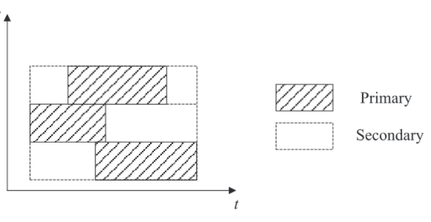
Figure 2.1: Example of opportunistic communications. Void area represent the spec-trum, i.e. the licensed users do not utilize.
can assign part of power to transmit the message of non-cognitive users. By proper power allocation at cognitive transmitter, the performance quality of non-cognitive receiver may keep the same or improve, and non-cognitive users transmit their own message simultaneously. Therefore, the overlay paradigm can improve the spectrum efficiency significantly.
3. Interweave Paradigm: The interweave paradigm can be referred as opportunis-tic communication, which is the original motivation of CR. The measurement by FCC shows that the licensed band is not utilized all the time. Therefore, the spectrum has many time and frequency holes in the licensed spectrum, which re-ferred to spectrum hole as shown in Fig. 2.1. The cognitive users can improve the spectrum efficiency by opportunistic communication when the non-cognitive users do not utilize the licensed spectrum. In the interweave paradigm, one needs to know the spectrum activity information of non-cognitive users. The cognitive transmitter requires spectrum sensing technique to obtain this side information.
2.2
Introduction to Convex Optimization
A general optimization problem can be expressed as
min f0(x)
s.t. fi(x) ≤ bi, i = 1, ..., m
(2.1)
where the vector x = [x1,· · · , xn]T is the optimization variable. The function f0 :
Rn → R is the objective function. The function f
i : Rn → R, i = i, · · · , m is the
constraint function. The constant b1,· · · , bm is the bounds for the constraints. ˆx
denotes the optimal solution of optimization problem(2.1). If the objective function and all constraints satisfy the following condition:
fi(αx + βy) = αfi(x) + βfi(y), i = 1, ..., m (2.2)
∀x, y ∈ Rn,∀α, β ∈ R
the optimization problem is called linear programming. If objective or any function is not linear, the optimization problem is called non-linear programming. Furthermore,
convex optimization problems mean that the objective and all constraints satisfy the
following conditions:
fi(αx + βy)≤ αfi(x) + βfi(y), i = 1, ..., m
α + β = 1 (2.3)
∀x, y ∈ Rn,∀α, β ∈ R and α > 0, β > 0
In general, the non-linear programming is difficult to solve. There is no ef-fective method to solve the general non-linear problem. However, some classes of non-linear optimization problems, such as least-squares problems and convex opti-mization problems, can be solved by efficient algorithms. There is in general no
analytical formula to solve the convex optimization problem. However, there is a very efficiency method, which is called the interior-point methods. The interior-point methods solve the problem in a short time even if the problem has thousands of vari-ables and constraints. Although the convex optimization can be solved via interior method easily, the transformation from the general non-linear problems to convex problems are very difficult. In general, many skills and tricks such as variable trans-formation and function composition are required.
Even if a non-linear optimization problem can not be transferred to convex easily, several heuristic techniques based on convex optimization can help solving non-convex optimization problems. Furthermore, convex optimization can find the bounds of non-convex optimization problem by replacing or relaxing to the convex constraints from the original problem.
2.3
Literature Survey
In this section, we categorize the related work about the beamforming and/or schedul-ing design for the sum rate maximization and transmit power minimization in the hierarchical underlying CR systems. The works of [5] and [9] focused on the trans-mit power minimization in the hierarchical underlying CR systems. The work [5] proposed a joint beamforming and power control algorithm to minimize the transmit power of secondary system under the constraint that the QoS requirement must be satisfied. However, the channel information between primary BS and users is difficult to obtain at a secondary BS since the cooperation between the primary and secondary users are required. In [9], the interference power constraint of the primary system was satisfied instead of the QoS constraint of the primary users. The work [9] proposed two suboptimal algorithms based on the least square and admission control.
The works [6–8] focused on the sum rate maximization. The work [6] proposed
a suboptimal joint beamforming and scheduling algorithm based on zero forcing beam-forming with equal power allocation and channel correlation between the primary and secondary users. However, the constraint of interference power to the primary system can not be satisfied in some cases. The work [7] develops a joint beamforming and power control iterative algorithm to sum rate maximization for fixed given serving set. However, the algorithm is only suitable in high SINR regime, which is not rea-sonable in interference-limited environment. A joint zero-forcing beamforming and user scheduling algorithm is proposed [8] to mitigate the the cross-tier interference. The scheduling in [8] includes both the primary and secondary users, but it is not practical for the primary users scheduling in the underlay CR systems. We compare our work with above research in Table 2.1.
Based on the above discussions, we can summarize that the problem of joint power allocation, beamforming and scheduling design to maximize the sum rate of the secondary CR system under the interference constraint has not been investigated well.
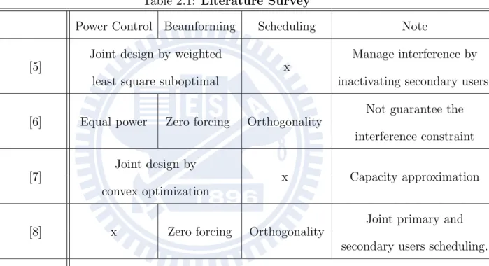
Table 2.1: Literature Survey
Power Control Beamforming Scheduling Note
[5]
Joint design by weighted
x
Manage interference by least square suboptimal inactivating secondary users.
[6] Equal power Zero forcing Orthogonality
Not guarantee the interference constraint
[7]
Joint design by
x Capacity approximation convex optimization
[8] x Zero forcing Orthogonality
Joint primary and secondary users scheduling.
Our works Joint design by convex optimization
12
CHAPTER 3
System Model and Problem Formulation
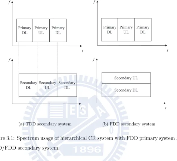
We consider a hierarchical underlying CR system, consisting of a primary system and secondary system. The primary system has a licensed spectrum. The secondary system is a multi-user broadcast system, which aims to provide services to secondary users under the condition that it can not interfere with the primary system. In the fourth generation (4G) of cellular wireless standards, the frequency division duplex (FDD) and time division duplex (TDD) are both considered. Therefore, what kind of duplexing modes of the primary and secondary is most suitable for hierarchical underlying CR system should be discussed. If the primary system is TDD, the sec-ondary system may interfere primary downlink and uplink in one transmission time for both TDD and FDD secondary systems as shown in Fig. 3.1. The interference to primary system would hardly be managed. If the primary system is FDD, the secondary systems can transmit at the primary downlink or uplink spectrum. The secondary system utilizing the uplink spectrum of primary users is a better option for two reasons. First, the quality of service (QoS) requirement of uplink is usually less strict than downlink. Thus, it may endure larger interference from secondary systems. Second, in order to cancel the interference, the channel state information (CSI) must be known at the secondary BS for utilizing downlink spectrum. In gen-eral, the CSI to the primary BS is more easily obtained than CSI to primary users.
Primary DL f Primary UL Primary DL f Secondary DL Secondary UL Secondary DL t t
(a) TDD secondary system
Secondary UL Secondary DL Primary DL f Primary UL Primary DL t f t (b) FDD secondary system
Figure 3.1: Spectrum usage of hierarchical CR system with FDD primary system and TDD/FDD secondary system.
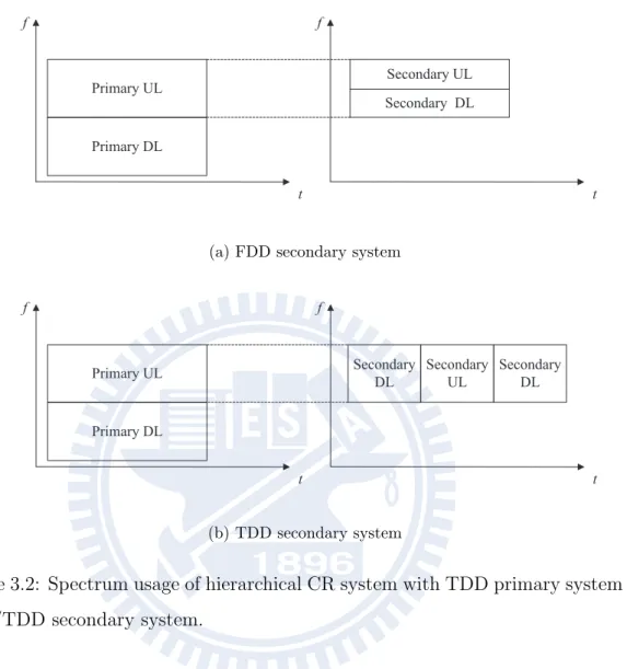
as shown in Fig. 3.2. Since the CSI between the primary and the secondary users are also required, TDD secondary system shown in Fig. 3.2(b) is preferable for the pur-pose of feedback. To summarize, FDD primary system and TDD secondary system utilizing the primary uplink spectrum is considered in the thesis.
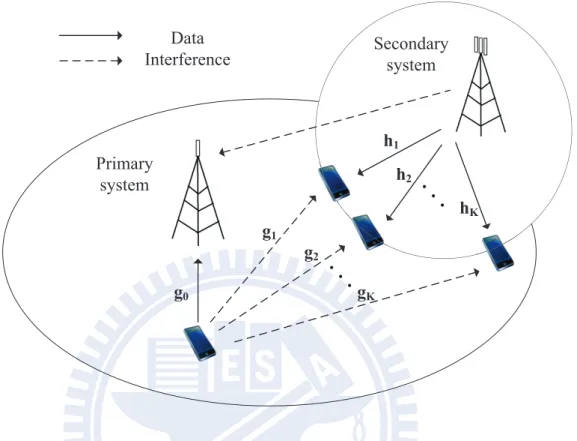
The hierarchical underlying CR system with FDD primary system and TDD secondary system is shown in Fig. 3.3. For simplification, assumes that only one primary utilizes the uplink band at a time. The primary BS, primary users and the secondary users are equipped with single antenna. The secondary BS are equipped with M . The secondary BS serve M secondary users at the most, which is selected
Secondary DL Secondary UL t f Primary UL t f Primary DL
(a) FDD secondary system
t f Secondary DL Primary UL t f Primary DL Secondary DL Secondary UL (b) TDD secondary system
Figure 3.2: Spectrum usage of hierarchical CR system with TDD primary system and FDD/TDD secondary system.
from K secondary users, where K > M . Both frequency non-selective and frequency selective fading channel are considered in the next section.
Primary system Secondary system g0 g1 g2 gK h1 h2 hK Data Interference
Figure 3.3: Hierarchical cognitive radio networks with a FDD primary system and a TDD secondary system, where the downlink spectrum of the secondary system utilizes the uplink spectrum of the primary system.
3.1
Single Carrier Hierarchical Cognitive Radio
Sys-tem
For a frequency non-selective channel, there is no inter-symbol interference (ISI). Thus, we may process the transmitted signal in the time domain, where sk and
x denote the transmitted signals from the secondary BS to the kth secondary user and the primary user to primary BS, respectively. An M × 1 vector wk represents
beamforming weight for the kth secondary user. S is the set of served users, where
S ⊆ {1, · · · , K}. The received signal of kth secondary user is rk = (w| {z }ksk)†hk desired signal + ( ∑ j∈S,j̸=k wjsj )† hk | {z }
intra−users interference
+ √| {z }Qgkx
inter−cell interference
+nk, k ∈ S , (3.1)
where hk denotes channel between M antennas of a secondary BS and the kth
sec-ondary user,√Q denotes the transmit power of the primary users, gk denotes channel
between primary user and kth secondary user, and nk is a Gaussian noise for kth
sec-ondary user with zero mean and variance σ2
N. We assume that the average power of
signal E[|sk|2
]
is normalized to one. Thus, the transmission power to the kth users
is ∥wk∥
2
. In addition, the received signal at the primary BS can be written as
r0 = √ Qg0x + ( ∑ j∈S wjsj )† h0 | {z }
inter−cell interference
+n0 , (3.2)
where n0 is the noise at the primary. Here, h0 represents channel between all the
served secondary users and the primary BS, g0 represents channel between primary
BS and primary user, and can be expressed as
gk= αkak, k = 1, ..., K (3.3)
hk= βkbkvk, k = 0, ..., K (3.4)
where αk and βk are the long-term fading, which includes pathloss exponent of four,
and log-normal shadow with standard deviation of 8 dB; ak and bk are short-term
Rayleigh fading, Note that vk is the steering vector which represent the relative phase
at each antenna
vk=
[
1, ejϕk,· · · , ej(M−1)ϕk]T (3.5)
where ϕk depends on the carrier frequency and propagation direction of the plane
For a hierarchical CR system, the interference to the primary system should be limited strictly. Therefore, we design beamforming weights to control the inter-cell interference (ICI) shown in (3.2) to be lower than a pre-defined threshold, while minimizing intra-use interference (IUI).
3.2
Multicarrier Hierarchical Cognitive Radio
Sys-tem
For the frequency selective channel, there are significant ISI due to multipath effects. The receive signals of the secondary users become
rk= (w| ks{zk)†hk,0} desired signal + Nd ∑ l=1 K ∑ j=1,j̸=k (wjsj)†hk,l | {z }
intra−users and inter−symbol interference
+ √| {z }Qgkx
inter−cell interference
+nk, k∈ S(3.6)
where Nd is number of paths in the frequency-selective channel; hk,l denotes channel
between secondary BS and kth secondary users in lth delay tap. Here we assume that
the channel from primary user is flat fading. hk,l and gk include the long-term fading
as in the previous section. Although beamforming may cancel IUI and ICI, there still is significant ISI. Orthogonal frequency division multiplexing (OFDM) can be used to reduce ISI. We may process the transmitted signal in the frequency domain by fast Fourier transform (FFT). Then, the received signal of the kth secondary user in the
nth
sc subcarrier can be expressed as
rk,nsc = ( ˜wk,nscs˜k,nsc) †h˜ k,nsc | {z } desired signal + ∑ jinSnsc,j̸=k ( ˜wj,nscs˜j,nsc) †h˜ k,nsc | {z }
intra−users interference
(3.7)
+ √| {z }Q˜gkx˜
inter−cell interference
+˜nk,nsc, k ∈ Snsc
where nsc = [1,· · · , Nsc]; Nsc is number of subcarriers; ˜hk,nsc denotes CSI for the k
th
secondary users in the nsc subcarriers; Snsc is the set of secondary users selected in
nthsc subcarrier. In addition, the received signal of the primary BS in the nthsc subcarrier can be expressed as r0 = √ Qg0x + Nsc ∑ nsc=1 ∑ j∈Snsc (wj,nscs˜j,nsc) †h 0,nsc | {z }
inter−cell interference
+n0 (3.8)
If there is no ISI, then we may design beamforming weights at each subcarrier to cancel the remaining interference.
3.3
Performance Metrics
3.3.1
System Sum Rate
We consider a multi-user broadcast system, and utilize Shannon capacity formula to model the system sum rate as follows:
Csum =
∑
k∈S
log2(1 + γk) , (3.9)
where S is the set of served users in each transmission; γk is the signal to interference
and noise ratio (SINR) of the kth user.
3.3.2
Fairness Index
Fairness is used to determine whether all the users share the resource fairly. There are several definitions of fairness. In this thesis, we utilize Jain’s fairness index as follows: F (x1, ..., xK) = ( 1 K K ∑ i=1 xi )2 1 K K ∑ i=1 x2 i = (∑K i=1 xi )2 K K ∑ i=1 x2 i , (3.10)
where xi is the number of resource allocating to the ith user; K is the number of
users. The larger the fairness index F is, the more the fair the resource allocate. The range of F is between K1 and 1. K1 is the worst case, which represents all resources are allocated to one user. If fairness index is equal to one, it represents that all users are allocated the same amount of resource.
3.4
Problem Formulation
Based on the signal model described in Sections 3.1 and 3.2, the single carrier trans-mission can be regarded as a special case in multicarrier transtrans-missions. Therefore, the following problems are formulated with multicarrier transmissions
The average SINR for the kth user in the jth subcarrier is given by
γk,j = w†k,jhk,j 2 K ∑ i∈Sj,i̸=k wi,j† hk,j 2 + Bk,j , (3.11) where K ∑ i∈Sj,i̸=k w†i,jhk,j 2
is the interference between secondary users with each other
in jth subcarrier. ∑K i∈Sj,i̸=k
wi,j† hk,j
2
can be regarded as the intra-user interference.
Q|gk,j|2 is the inter-cell interference resulted from the primary user, and σN2 is the
thermal noise. The inter-cell interference resulted from the primary user can not be controlled at the secondary BS. Noise can be combined with the inter-cell interference as Bk,j = Q|gk,j|2+ σN2,∀k, which is a constant to the secondary users in each
trans-mission. Since Sj includes unknown users, we introduce a new variable bj, regarded
to the scheduling parameter. If the ith secondary is served in the jth subcarrier, b i,j
is equal to one; otherwise, bi,j is equal to zero. The relationship between Sj and bj
can be written as
Sj ={bi,j|bi,j = 1, i = 1, ..., K} (3.12)
Then, the system sum rate can be formulated as follows: Csum = max b,W1,...,WNsc Nsc ∑ j=1 K ∑ k=1 log2 1 + bk,j wk,j† hk,j 2 K ∑ i∈Sj,i̸=k bi,j wi,j† hk,j 2 + Bk,j , (3.13)
where Wj = [w1,j,· · · , wK,j] is the beamforming weight matrix in the jth subcarrier.
The subcarriers assigned to kth secondary user are {j |b
k,j = 1, j = 1, ..., Nsc}, and
the number of users served in the jthsubcarrier is ∑K i=1
bi,j, which must be smaller than
or equal to M . Therefore, (3.13) can be regarded as the secondary system sum rate after user selection and subcarrier allocation. Our goal is to maximize the sum rate of the secondary system subject to three constraints:
1. The interference power to the primary BS is strictly limited to a pre-defined thresh-old.
2. The number of served users in each transmission must be smaller than M in each subcarrier.
3. The transmit power from secondary BS is limited.
Thus, the sum rate maximization problem can be formulated as follows:
max b,W1,...,WNsc Nsc ∑ j=1 K ∑ k=1 log2 1 + bk,j w†k,jhk,j 2 K ∑ i∈Sj,i̸=k bi,j w†i,jhk,j 2 + Bk,j , subject to (C.1) K ∑ i=1 bi,j wi,j† h0,j 2 ≤ Imax ; (3.14)
(C.2) K ∑ i=1 bi,j ≤ M, ∀j = 1, ..., Nsc; (C.3) Nsc ∑ j=1 K ∑ i=1
bi,j∥wi,j∥2 ≤ Pmax;
(C.4)bi,j ∈ {0, 1} , ∀i = 1, . . . , K, j = 1, ..., Nsc ,
where Imax and Pmax are the interference power and transmission power constrain,
respectively. In (C.2), one dimension of antenna domain should be used to cancel the interference to the primary BS Thus, secondary BS can only serve M − 1 users in each transmission at most. However, if proper user set is selected or the interference constraint is not too strict, secondary BS may serve M users at a time. In the objective function of (3.14), we jointly design beamforming weight W and scheduling parameter b to maximize the sum rate of the secondary BS with transmit power constraint (C.3). Note that the transmit power to the ith secondary user in the jth subcarrier is∥wi,j∥
2
. Therefore, (C.3) also implies that power allocation is not only to each secondary user but also for subcarriers. Hence, (3.14) can be regarded as a joint optimization problem for multi-user beamforming, power allocation and scheduling in a system with multiple subcarriers.
22
CHAPTER 4
Joint Power allocation, Beamforming and
Scheduling Design in Hierarchical
Cognitive Radio System with
Multi-carrier Transmissions
In this chapter, we present a joint power allocation, beamforming and scheduling design to maximize the sum rate of the secondary BS in a hierarchical CR system. We consider the multicarrier transmissions. The sum rate maximization problem is transferred from a MINLP to a convex problem, and an iterative algorithm is proposed to determine the optimal power allocation, beamforming weight and user scheduling.
4.1
Convexity of Optimization Problem
The optimization problem (3.14) is non-trivial for following two reasons:
1. Two variables W and b are continuous and discrete, respectively. It is called mixed integer non-linear optimization problem (MINLP), which is hard to solve. Although branch and bound (BnB) is a known method to solve mixed integer
2. The objective is neither concave nor convex function respect to W Therefore, the maximization problem can not be solved by convex optimization even if we assume the optimal b is known.
In this section, we attempt to simplify and reformulate the non-convex optimization problem (3.14) to a convex optimization problem.
First, check whether each variable and constrain are necessary. Then, two observations are made as follows:
1. For the sum-rate maximization purpose, non-served users should not be allocated power. Thus, the variable b can be dropped, and we can utilize ∥wi∥
2
, which is transmit power allocated to ith secondary user, to represent scheduling instead
of bi, where bi = 0 and bi = 1 corresponding to ∥wi∥2 = 0 and ∥wi∥2 > 0,
respectively.
2. As shown in (C.2) of (3.14), the number of served users at a time must be not larger than M . Otherwise, the beamforming weight matrix W can not null the inter-user interference. We can expect that the rank of optimal beamforming weight matrix ˆW must be smaller than or equal to M . Then, (C.2) in (3.14) can
be dropped.
After the above simplifications, the optimization problem (3.14) can be reformulated as follows: max W1,...,WNsc Nsc ∑ j=1 K ∑ k=1 log2 1 + w†k,jhk,j 2 K ∑ i=1,i̸=k wi,j† hk,j 2 + Bk,j , subject to 23
(C.1) K ∑ i=1 w†i,jh0,j 2 ≤ Imax; (4.1) (C.2) Nsc ∑ j=1 K ∑ i=1 ∥wi,j∥2 ≤ Pmax.
Now, (C.1) and (C.2) are norm square and quadratic form, respectively. Both of them are convex functions. However, the objective function is logarithm of quadratic-over-quadratic, which is not a concave function. If capacity log2(1+SINR) is approximated by log2(SINR), the problem can be solved by convex optimization with an iterative algorithm in [7]. However, this assumption does not make sense in our problem, since SINR of non-served users are zero. In the next section, the semi-definite relaxation approaches are applied to this problem.
4.2
Semi-Definite Relaxation Approach
By linear algebra, we know that T r(AB) = T r(BA) for arbitrary matrix A and B. The quadratic form can be expressed to the form of trace function as:
w†k,jhk,j
2
= (w†k,jhk,j)(w†k,jhk,j)∗ = T r(wk,j† hk,jh†k,jwk,j) (4.2)
= T r(wk,jwk,j† hk,jh†k,j)
This equation is affine respect to matrix wk,jwk,j† . Thus, new variables are introduced
Hk,j = hk,jh†k,j,∀k ∈ [0, K], j ∈ [1, Nsc] (4.3)
and
Wk,j = wk,jw†k,j,∀k ∈ [1, K], j ∈ [1, Nsc] (4.4)
Then, (4.2) can be expressed as:
Then, (4.1) can be transformed to the following equivalent problem: max W1,1,··· ,W1,Nsc,W2,1,··· ,WK,Nsc Nsc ∑ j=1 K ∑ k=1 log2[1 + T r(Wk,jHk,j) K ∑ i=1,i̸=k T r(Wi,jHk,j) + Bk,j ] , subject to (C.1) K ∑ k=1 T r(Wk,jH0,j)≤ Imax ; (4.6) (C.2) Nsc ∑ j=1 K ∑ k=1 T r(Wk,j)≤ Pmax; (C.3)Wk,j ≽ 0, ∀k ∈ [1, K], j ∈ [1, Nsc] ; (C.4)Rank(Wk,j) = 1,∀k ∈ [1, K], j ∈ [1, Nsc] ,
where Wi,j denotes the beamforming weight for the ith secondary user in the jth
subcarrier. The problem is a semi-definite programming since all variables are rank one hermitian symmetric positive semi-definite matrix. Note that the rank constrain (C.4) is not convex. Hence, we relax (C.4) as well to obtain the following problem:
max W1,1,··· ,W1,Nsc,W2,1,··· ,WK,Nsc Nsc ∑ j=1 K ∑ k=1 log2[ T r(Wk,jHk,j) + K ∑ i=1,i̸=k T r(Wi,jHk,j) + Bk,j K ∑ i=1,i̸=k , T r(Wi,jHk,j) + Bk,j ] subject to (C.1) K ∑ k=1 T r(Wk,jH0,j)≤ Imax; (4.7) (C.2) Nsc ∑ j=1 K ∑ k=1 T r(Wk,j)≤ Pmax; (C.3)Wk,j ≽ 0, ∀k ∈ [1, K], j ∈ [1, Nsc] . 25
Now, all constrains are convex, but the objective function is still non-concave. The objective function is the composition of logarithm and linear fractional function, which does not grantee a concave function with respect to Wk,j,∀k, j. In order to transform
the objective function to a concave function, we introduce additional variable
Ω = Ω1,1 · · · Ω1,Nsc .. . . .. ... ΩK,1 · · · ΩK,Nsc , (4.8)
where Ω is the upper bound of intra-user interference power among all secondary users. Then, the optimization problem can be reformulated as:
max W1,1,··· ,W1,Nsc,W2,1,··· ,WK,Nsc Nsc ∑ j=1 K ∑ k=1 log2[ T r(Wk,jHk,j) + K ∑ i=1,i̸=k T r(Wi,jHk,j) + Bk,j K ∑ i=1,i̸=k T r(Wi,jHk,j) + Bk,j ] , subject to (C.1) K ∑ k=1 T r(Wk,jH0,j)≤ Imax; (4.9) (C.2) Nsc ∑ j=1 K ∑ k=1 T r(Wk,j)≤ Pmax; (C.3)Wk,j ≽ 0, ∀k ∈ [1, K], j ∈ [1, Nsc] ; (C.4) K ∑ i=1,i̸=k T r(Wk,jHk,j)≤ Ωk,j,∀j = 1, ..., Nsc ,
where Ωk,j,∀k, j are variables with non-negative values bounding the intra-user
the single carrier case as: max W1,1,··· ,WK, K ∑ k=1 log2[ T r(Wk,jHk) + K ∑ i=1,i̸=kT r(WiHk) + Bk K ∑ i=1,i̸=k T r(WiHk) + Bk ] , subject to (C.1) K ∑ k=1 T r(WkH0)≤ Imax ; (4.10) (C.2) K ∑ k=1 T r(Wk)≤ Pmax; (C.3)Wk ≽ 0, ∀k ∈ [1, K] ; (C.4) K ∑ i=1,i̸=k T r(WkHk)≤ Ωk .
For any fixed Ω, (4.9) is a concave maximization problem, denoted by R1(Ω).
The optimal solution [ ˆW1,· · · , ˆWk] of the convex problem (4.9) can be solved
by toolbox CVX [16]. Then, one need to check the rank of the solution ˆW =
[ ˆW1,· · · , ˆWk]. If all of them are one, it means that we do not relax any constraints.
ˆ
W will also be the optimal solution of the original problem (4.1), if the optimal ˆΩ is
known. In addition, the optimal user scheduling and subcarrier assignment are:
ˆ
Sj ={k |Rank(Wk) = 1, k = 1, ..., K}, ∀j = 1, · · · , Nsc (4.11)
Then, the globally optimal beamforming weightWˆk,j,∀k, j of (4.10) can be converted
into a feasible solution by ˆWk,j = ˆwk,jwˆk,j† ,∀k ∈ ˆSj, j = [1,· · · , Nsc]. If the rank of
any Wk,j,∀k, j is larger than one, we must extract a feasible vector wk,j from Wk,j,
which is usually not an optimal solution. Fortunately, the rank of ˆWk,j,∀k, j is always
smaller than or equal to one in our simulation experience.
4.3
Iterative Sum-Rate Maximization Algorithm
Although the optimal ˆΩ can be obtained by the exhaustive search, we still prefer
to develop an efficient algorithm to obtain ˆΩ to reduce search space. In (C.4) of
(4.9), the power allocation is across the subcarrier. Thus, the optimal beamforming weight in each subcarrier is correlated with others. A simplified formulation is first considered as: max W1,1,··· ,W1,Nsc,W2,1,··· ,WK,Nsc K ∑ k=1 log2[ T r(Wk,jHk,j) + K ∑ i=1,i̸=k T r(Wi,jHk,j) + Bk,j K ∑ i=1,i̸=k T r(Wi,jHk,j) + Bk,j ] , subject to (C.1) K ∑ k=1 T r(Wk,jH0,j)≤ Imax; (4.12) (C.2) K ∑ k=1 T r(Wk,j)≤ Pmax Nsc ,∀j ∈ [1, Nsc] ; (C.3)Wk,j ≽ 0, ∀k ∈ [1, K], j ∈ [1, Nsc] ; (C.4) K ∑ i=1,i̸=k T r(Wk,jHk,j)≤ Ωk,j,∀j = 1, ..., Nsc,
where (C.2) represents equal power allocation over all subcarriers. Then, the power allocation, beamforming and scheduling in each subcarrier is independent with other subcarriers. That is, Ωj = [Ω1,j,· · · , ΩK,j]T can change without impacting other
subcarrier. Therefore, an iterative algorithm can be developed for the single car-rier transmission, and may apply to multicarcar-rier transmission by utilizing to each subcarrier.
The following formulations are expressed as single carrier transmission. First, we define:
R2(W, Ω) = K ∑ k=1 {log2[T r(WkHk) + K ∑ i=1,i̸=k T r(WiHk) + Bk] − log2[Ωk+ Bk]} (4.13) = g(W) + f (Ω) , where g( ¯W) = log2[T r(WkHk) + K ∑ i=1,i̸=k T r(WiHk) + Bk] f (Ω) = −log2(Ωk+ Bk) .
Then, the optimization problem is formulated about Ω as follows:
R1(Ω) = max
W∈Θ(W)R2(W, Ω) (4.14)
where Θ(W) is the feasible set with respect to (4.9). Note that the size of set Θ depends on the value of Ω. In (C.4) of (4.9), if Ω becomes smaller, the set of available beamforming weight W would become smaller. Consider two vector Ω(1) =
[Ω(1)1 ,· · · , Ω(1)K ] and Ω(2) = [Ω(2)
1 ,· · · , Ω (2)
K ], corresponding to two non-empty set Θ(1)
and Θ(2), respectively. Assume that Ω(2) ≼ Ω(1),i.e.,Ω(2)k ≤ Ω(1)k ,∀k. The following
observations can be made:
1. f (Ω(2))≥ f(Ω(1)).
2. max
W∈Θ(2)g(W)≤ maxW∈Θ(1)g(W), since Θ
(2) is a subset of Θ(1).
The first observation shows that the system sum rate can be improved by decreasing
Ω, but the second observation seems to reveal opposite trend as Ω decrease.
There-fore, we take a simple example to investigate the relationship between sum rate and Ω.
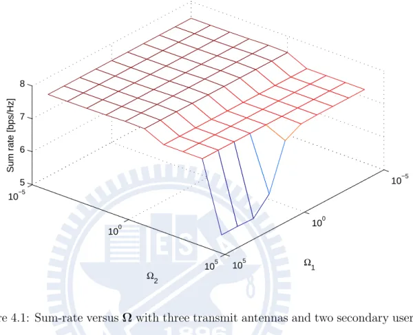
10−5 100 105 10−5 100 105 5 6 7 8 Ω1 Ω2 Sum rate [bps/Hz]
Figure 4.1: Sum-rate versus Ω with three transmit antennas and two secondary users
Assumes that the number of transmit antennas is three, and there are two secondary users. As shown in Fig. 4.1, the secondary system sum rate increases significantly by decreasing Ω = [Ω1, Ω2] when both Ω1 and Ω2 are large. However, the optimal
value does not occurs at the boundary, which can be seen more clearly in Fig. 4.2 and Fig4.3. If Ω decreases without restrictions, the sum rate can always be not improved. Note that if Ω is set to be zero, the solution will become zero-forcing beamforming, which is usually not an optimal solution. To summarize, the system sum rate can be improved by decreasing the intra-user interference power constraint for those users in serving set Ωk, k∈ S, but Ωk can not be too small.
10−6 10−4 10−2 100 102 104 7.2 7.25 7.3 7.35 7.4 7.45 7.5 7.55 Sum Rate [bps/Hz] Ω1
Figure 4.2: Sum-rate versus Ω with three transmit antennas and two secondary users, and fixed Ω2.
of the secondary system. The entire procedures of the iterative algorithm are shown in Fig. 4.4. First, we initialize i = 1 and k = 1, which corresponds iterative loop and user index, respectively. In order to not restrict the intra-user interference to those non-served users, the feasible set Ω(0) is set to a sufficiently large non-negative real
value. Then, we solve (4.10), and check whether initial Ω(0) is feasible. Second, we
choose a constant step size δ, where 0 < δ < 1, and update Ω(i−1) to Ω(i) by
Ω(i) = Ω(i−1)− (1 − δ)Ω(i)k ek . (4.15)
where ek is the kth column of a K× K identity matrix IK. Then, we solve (4.10) for
new Ω(i) and check whether the system sum rate improvement R1(Ω(i))− R1(Ω(i−1))
10−6 10−4 10−2 100 102 104 5 5.5 6 6.5 7 7.5 Ω2 Sum Rate [bps/Hz]
Figure 4.3: Sum-rate versus Ω with three transmit antennas and two secondary users, and fixed Ω1.
is larger than a pre-defined threshold ∆r ≥ 0, which is a small constant value. If so,
set i = i + 1 and continue to decrease Ωk until the capacity improve insignificantly.
Otherwise, set Ω(i) = Ω(i−1), R1(Ω(i)) = R1(Ω(i−1)) and ˆW(i) = ˆW(i−1), and decrease
the intra-user interference to the next secondary user until k = K. Now, we have the optimal beamforming ˆW = [ ˆW1,· · · , ˆWK], which includes rank one and zero
matrix. The serving set ˆS includes the users with rank 1 solution, where the size of S is smaller than or equal to than the number of transmit antennas M . Although an
iterative algorithm is utilized to find the optimal Ω, there is still an error compared with the optimal solution. The margin of this error depends on the step size δ and the number of secondary users. This error may increase as the number of secondary
users K increase. Therefore, the users, who are not in the serving set S, can be dropped and set K = |S|, where |·| denotes the size of a set. Again, we run the iterative algorithm for users in S. Note that it may still have a zero matrix solution for some users, which means the number of served users may be smaller than|S|. In the next chapter, numerical results with the single and multiple carrier transmissions are shown. The results of multicarrier transmissions are obtained by executing the iterative algorithm shown in Fig. 4.4 for each subcarrier.
(0) Set to a large number Initialzation W ( ) ( 1) ( 1) Choose 0 1 (1 ) i i i q q Update d d - -< < = - -W W W e ( ) ( ) 1 . ˆ Find ( i ) and i Convex Opt R W W Set i= +i 1 Yes ( ) ( 1) ( ) ( 1) 1 1 ( ) ( 1) Set ( ) ( ) ˆ ˆ i i i i i i R R -= = = W W W W W W No Set 1 1 i i k k = + = + k<K Yes (0) Set to a large number Initialzation W ( ) ( 1) ( 1) 0 1 (1 ) i i i q q Update Choose e d d - -< < W = W - - W ( ) ( ) 1 . ˆ Find ( i) and i Convex Opt R W W Set i= +i 1 ŚŦŴ ( ) ( 1) ( ) ( 1) 1 1 ( ) ( 1) Set ( ) ( ) ˆ ˆ i i i i i i R R -= = = W W W W W W Set 1 1 i i k k = + = + k<K Yes ( ) ( 1) 1( ) 1( ) i i r R W -R W - > D
Find the serving set S,
which is secondary users
with largest rate and set M K=M No Stop No ( ) ( 1) 1( ) 1( ) i i r R W -R W - > D No
35
CHAPTER 5
Numerical Results and Discussion
5.1
Single Carrier Case
5.1.1
Simulation Assumptions
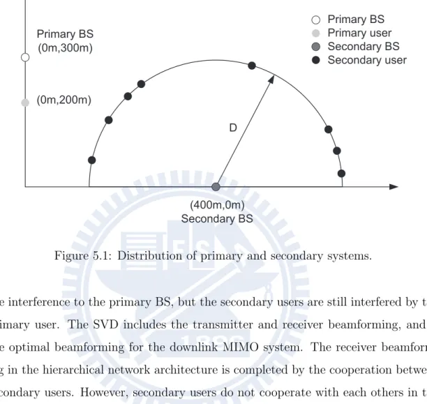
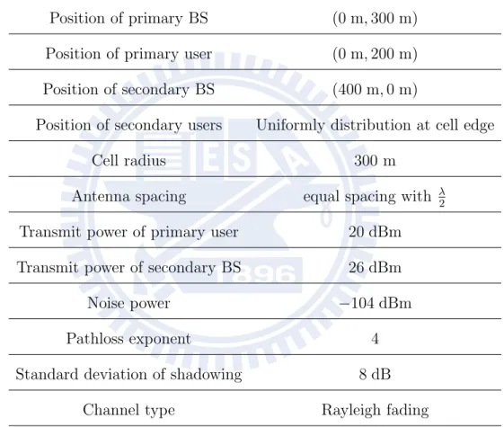
In this subsection, we describe the simulation environments for evaluating the per-formance of the proposed iterative algorithm. The distribution of the primary and secondary systems are shown in Fig. 5.1. Assume that the primary and secondary BS are located at (0 m, 300 m) and (400 m, 0 m), respectively. The radius of the secondary system is 300 m. In a primary user with fixed location (0 m, 200 m), K secondary users are uniformly distributed at the secondary cell edge. The secondary BS equipped with M transmit antennas which are equal spacing with half a wave-length. Assume that the CSI is perfectly known at the secondary BS. The transmit power of the primary user and secondary BS are 20 dBm and 26 dBm, respectively. The noise power is −104 dBm. The pathloss exponent is four and the standard de-viation of shadowing is 8 dB in both primary and secondary system. Simulation parameters are listed in Table 5.1.
There are two schemes for comparison: the first scheme is zero forcing beam-forming between primary BS and M−1 secondary users with the exhausted scheduling and the optimal power allocation, which is regarded as a lower bound. Another scheme is singular value decomposition (SVD) to the secondary users, and does not control
Primary BS Primary user Secondary BS Secondary user (400m,0m) Secondary BS Primary BS (0m,300m) D (0m,200m)
Figure 5.1: Distribution of primary and secondary systems.
the interference to the primary BS, but the secondary users are still interfered by the primary user. The SVD includes the transmitter and receiver beamforming, and is the optimal beamforming for the downlink MIMO system. The receiver beamform-ing in the hierarchical network architecture is completed by the cooperation between secondary users. However, secondary users do not cooperate with each others in the proposed algorithm. Thus, the SVD scheme can be regards as an upper bound.
5.1.2
Effects of Number of Transmit Antennas
Fig. 5.2 shows that the sum rate versus the number of the secondary BS transmit antennas for three beamforming and scheduling schemes. We can observe that the proposed scheduling scheme has significant improvement compared with the zero-forcing scheme. The gain comes from allowing some interference power to the primary
Table 5.1: Simulation Parameters for Single Carrier Transmissions Position of primary BS (0 m, 300 m)
Position of primary user (0 m, 200 m) Position of secondary BS (400 m, 0 m)
Position of secondary users Uniformly distribution at cell edge
Cell radius 300 m
Antenna spacing equal spacing with λ2 Transmit power of primary user 20 dBm Transmit power of secondary BS 26 dBm
Noise power −104 dBm
Pathloss exponent 4
Standard deviation of shadowing 8 dB
Channel type Rayleigh fading
3 4 5 4 5 6 7 8 9 10 11 12 13
Number of transmit antennas
Spectral efficiency (bps/Hz)
Proposed algorithm ZF with optimal scheduling SVD with optimal scheduling
Figure 5.2: Sum rate for various numbers of transmit antennas, where the number of the secondary users is 10, and Imax = 10 dBm.
BS in our algorithm. However, interference power to the primary BS is zero. In addition, the proposed algorithm may serve M users in each transmission, but the zeor-forcing scheme served M−1 users fixedly. Shannon capacity formula is logarithm function, and the low SINR region can be regarded as the linear region. Thus, one more user can be served may lead to significant improvement.
5.1.3
Effects of Maximal Allowable Interference to Macro
Cell
Fig. 5.3 shows that the sum rate versus the maximal allowable interference to pri-mary BS Imax for the three considered beamforming and scheduling schemes. The
always forces the interference to zero. Thus, the sum rate of these two schemes will not change as Imax changes. However, our algorithm increase significantly as Imax
increases. It means that our proposed scheme is very flexible for different interfer-ence constraints Imax. As Imax increases, the sum rate of the proposed algorithm
will gradually approach to the SVD scheme. Nevertheless, they will not have the same performance even if Imax goes infinity because of the received beamforming of
SVD scheme. As Imax decreases, the sum rate of the proposed algorithm will
grad-ually approach to the zero-forcing scheme. In fact, the proposed algorithm and the zero-forcing scheme will have the same performance as Imax approach to the negative
infinity. However, the proposed algorithm can improve capacity significantly when
Imax is large. Note that Imax will affect the coverage and transmit power of the
secondary BS. Thus, the adaption of Imax is very important for the underlying CR
system.
5.1.4
Effects of Number of Cognitive Radio Users
Fig. 5.4 shows the sum rate versus the number of the secondary users for three beam-forming and scheduling schemes. The slope of the proposed algorithm is same as the SVD scheme, and larger than zero-forcing scheme. Thus, the user diversity of the proposed algorithm is same as the exhausted scheduling.
5.2
Multicarrier Case
5.2.1
Simulation Assumptions
In this subsection, we describe the simulation environment for evaluating the perfor-mance of the proposed iterative algorithm. The distribution of primary and secondary systems are shown in Fig. 5.5. Assumes that the primary and secondary BS are
−8 −6 −4 −2 0 2 4 6 8 10 4 5 6 7 8 9 10 11
Maximal allowable interference to primary BS (dB)
Spectral efficiency (bps/Hz)
Proposed algorithm ZF with optimal scheduling SVD with optimal scheduling
Figure 5.3: Sum rate for various numbers of maximal allowable interference to primary BS, where the number of transmit antennas is three, and the number of the secondary users is 10.
cated at (0 m, 300 m) and (400 m, 0 m), respectively. The radius of the secondary system is 300 m. There is a primary user with a fixed location (0 m, 200 m), and K secondary users are located fixedly at the secondary cell edge with equal separation. The secondary BS equipped with M transmit antennas which are equal spacing with half a wavelength. Assume that the CSI is perfectly known at secondary BS. The transmit power of the primary user is 20 dBm. The transmit power of secondary BS in each subcarrier is 20 dBm The noise power is −110 dBm in each subcarrier. The pathloss exponent is four and the standard deviation of shadowing is 8 dB in both primary and secondary systems. The frequency-selective channel is i.i.d. Rayleigh fading in each sub-carrier. The summary of simulation parameters are shown in
5 6 7 8 9 10 11 12 13 14 15 2 3 4 5 6 7 8 9 10 11 12
Number of secondary users
Spectral efficiency (bps/Hz)
Proposed algorithm ZF with optimal scheduling SVD with optimal scheduling
Figure 5.4: Sum rate for various numbers of secondary users, where the number of transmit antennas is three , and Imax = 10 dBm.
Table 5.2.
5.2.2
Fairness Compared with Single Carrier Transmissions
Fig. 5.6 shows the fairness index versus the number of subcarrier. Although the fairness is poor in single channel transmission, the fairness index improve significantly as the number of subcarriers increase. The fairness index is 0.93 for 8 subcarriers. Thus, the secondary BS can still serve users fairly on multicarrier transmissions even if the proposed algorithm is in order to maximize system sum rate.
Table 5.2: Simulation Parameters for Multicarrier Transmissions Position of primary BS (0 m, 300 m)
Position of primary user (0 m, 200 m)
Position of secondary BS (400 m, 0 m)
Position of secondary users
Fixed location at cell edge with equal separation.
Cell radius 300 m
Antenna spacing equal spacing with λ2 Transmit power of primary user 20 dBm
Transmit power of secondary BS 20 dBm in each subcarrier
Noise power −110 dBm in each subcarrier.
Pathloss exponent 4
Standard deviation of shadowing 8 dB
Primary BS Primary user Secondary BS Secondary user (400m,0m) Secondary BS Primary BS (0m,300m) D (0m,200m)
Figure 5.5: Distribution of primary and secondary systems.
1 2 3 4 5 6 7 8 0.74 0.76 0.78 0.8 0.82 0.84 0.86 0.88 0.9 0.92 0.94 Number of sub−channel Fairness index
Figure 5.6: Fairness index for different number of transmit antennas.
44
CHAPTER 6
Conclusions
In this thesis, we developed a joint power allocation, transmitted beamforming and user scheduling design for the hierarchical cognitive radio networks in both frequency selective and frequency non-selective fading channel. SDR is applied to transfer the MINLP joint design problem to a convex problem. The numerical results show the performance for different numbers of antennas, secondary users and maximal allow-able interference power to the primary system. The improvement of the sum rate saturates when a large number of transmit antennas, even the scheduling is consid-ered jointly. The proposed algorithm is very flexible for different interference power constraints. The sum rate of the secondary system improve significantly as the inter-ference power constraint becomes less strict, which is contributed by joint beamform-ing and schedulbeamform-ing design. The user diversity of the proposed algorithm is the same as the exhausted scheduling. Therefore, the scheduling of the proposed algorithm is approaching to the optimal value.
Our proposed algorithm can also be applied to the multicarrier transmissions. The proposed algorithm is designed for the sum rate maximization. Although, the fairness of the proposed is not the main design goal, users can be served quite fairly as the proposed algorithm is applied to the multicarrier transmissions.
45
Bibliography
[1] FCC Spectrum Policy Task Force, “Report of the spectrum efficiency working group,” Technical Report 02-135, Tech. Rep., 2002.
[2] S. Haykin, “Cognitive radio: brain-empowered wireless communications,” IEEE
Journal on Selected Areas in Communications, vol. 23, no. 2, pp. 201 – 220, feb.
2005.
[3] N. Devroye, M. Vu, and V. Tarokh, “Cognitive radio networks,” IEEE Signal
Processing Magazine, vol. 25, no. 6, pp. 12 –23, november 2008.
[4] A. Goldsmith, S. Jafar, I. Maric, and S. Srinivasa, “Breaking spectrum gridlock with cognitive radios: An information theoretic perspective,” Proceedings of the
IEEE, vol. 97, no. 5, pp. 894 –914, may 2009.
[5] H. Islam, Y.-C. Liang, and A. T. Hoang, “Joint beamforming and power control in the downlink of cognitive radio networks,” in IEEE Wireless Communications
and Networking Conference, 2007.WCNC 2007., march 2007, pp. 21 –26.
[6] K. Hamdi, W. Zhang, and K. Ben Letaief, “Joint beamforming and scheduling in cognitive radio networks,” in IEEE Global Telecommunications Conference,
2007. GLOBECOM ’07., nov. 2007, pp. 2977 –2981.
[7] M.-L. Ku, L.-C. Wang, and Y.-T. Su, “Optimal multiuser beamforming and power allocation for hierarchical cognitive radio systems,” in IEEE Information
Theory and its Applications (ISITA), 2010 International Symposium on, oct.
2010, pp. 946 –951.
[8] W. Zong, S. Shao, Q. Meng, and W. Zhu, “Joint user scheduling and beamform-ing for underlay cognitive radio systems,” in APCC 15th Asia-Pacific Conference
on Communications, oct. 2009, pp. 99 –103.
[9] H. Islam, Y.-C. Liang, and A. T. Hoang, “Distributed power and admission con-trol for cognitive radio networks using antenna arrays,” in IEEE International
Symposium on New Frontiers in Dynamic Spectrum Access Networks, 2007. DyS-PAN 2007. 2nd, april 2007, pp. 250 –253.
[10] M. Costa, “Writing on dirty paper (corresp.),” IEEE Transactions on
Informa-tion Theory, vol. 29, no. 3, pp. 439 – 441, may 1983.
[11] F. Rashid-Farrokhi, L. Tassiulas, and K. Liu, “Joint optimal power control and beamforming in wireless networks using antenna arrays,” IEEE Transactions on
Communications, vol. 46, no. 10, pp. 1313 –1324, oct 1998.
[12] W. Yu and T. Lan, “Transmitter optimization for the multi-antenna downlink with per-antenna power constraints,” IEEE Transactions on Signal Processing, vol. 55, no. 6, pp. 2646 –2660, june 2007.
[13] T. Yoo and A. Goldsmith, “On the optimality of multiantenna broadcast schedul-ing usschedul-ing zero-forcschedul-ing beamformschedul-ing,” IEEE Journal on Selected Areas in
Com-munications, vol. 24, no. 3, pp. 528 – 541, march 2006.
[14] E. Matskani, N. Sidiropoulos, Z. quan Luo, and L. Tassiulas, “Convex approxi-mation techniques for joint multiuser downlink beamforming and admission con-trol,” IEEE Transactions on Wireless Communications, vol. 7, no. 7, pp. 2682 –2693, july 2008.
[15] K. Cumanan, R. Krishna, L. Musavian, and S. Lambotharan, “Joint beamform-ing and user maximization techniques for cognitive radio networks based on branch and bound method,” IEEE Transactions on Wireless Communications, vol. 9, no. 10, pp. 3082 –3092, october 2010.
[16] M. Grant and S. Boyd, “CVX: Matlab software for disciplined convex program-ming, version 1.21,” http://cvxr.com/cvx, Apr. 2011.
Vita
Yu-Jung Liu
He was born in Taiwan, R. O. C. in 1987. He received his B.S. at the De-partment of Communication Engineering, National Chiao-Tung University in 2009. From July 2009 to August 2011, he worked his Master degree in the Mobile Commu-nications and Cloud Computing Lab at the Institute of Communication Engineering at National Chiao-Tung University. His research interests are in the field of wireless communications.