VOL. 36, NO. 3 AMERICAN WATER RESOURCES ASSOCIATION JUNE 2000
COMPARATWE STUDY OF DROUGHT PREDICTION
TECHNIQUES FOR RESERVOIR OPERATION'
Ke-Sheng Cheng, Hui-Chung Yeh, and Ching-Yuan Liou2
ABSTRACT: Predicting the likelihood of a drought markedly enhances the efficiency of reservoir operations. This study applies the kriging method and time series analysis to predict inflows to Shihmen Reservoir in northern Taiwan. A subsequent reservoir operation simulation is employed to determine the drought lead time (DLT), the time before the onset of a drought. A more efficient
reservoir operational strategy can be established with the aid of DLT and the probability of successful drought prediction (Ps). Sim-ulation results of reservoir operation over a period of three decades demonstrate that, at one month DLT, the kriging approach achieves 0.86 of Ps for moderate droughts and 0.94 of Ps for severe droughts. The kriging approach generally outperformed the time series approach in terms of DLT, Ps of drought prediction, and the num-ber of correctly predicted drought events.
(KEY TERMS: drought; drought lead time; kriging; time series analysis; modeling/statistics.)
INTRODUCTION
Drought is a natural phenomenon. There have been many different definitions and identification methods of drought in the literature. Rossi et al.
(1992) thoroughly reviewed the methodologies for estimating and analyzing regional drought. Droughts can generally be classified as: (1) a meteorological drought, which occurs when rainfall is far below the normal amount for a significant period of time; (2) an agricultural drought, which occurs when soil moisture is depleted to the extent that crop and pasture yields
are significantly affected; and (3) a hydrological
drought, which occurs when water resources cannot
adequately supply established users under a given
water management scheme. Bonacci (1993) applied
three methods of drought identification, i.e., run
analysis, a discrete Markov process, and the
per-centile method, to a series of monthly rainfall data. Drought is also a continuous process, possibly last-ing for a long or short period of time. Thus, durlast-ing a drought, the waiting period before taking any remedi-al measures is of concern for reservoir operators. The
timing associated with remedial actions must be clearly and precisely defined. For this purpose, an
indicator of an approaching drought that will prompt immediate remedial actions is desired. Rouhani and Cargile (1989) proposed a geostatistical indicator for an approaching drought. Geostatistical estimation,
also known as kriging, was employed to predict streamfiows during low-flow periods in a drought
prone area. Drought lead time (DLT), defined as the
time length from the present to the onset of an
approaching drought, was calculated and used as an indicator for drought management.The average annual rainfall in Taiwan is
abun-dant, i.e., 2,500 mm, as compared to the global
aver-age of 970 mm. However, over 75 percent of the
annual rainfall occurs during the wet season (from
May to October). Typhoons usually occur in July,
August, and September, bringing much of the needed rainfall for the coming dry season (from November to April), during which an enormous amount of water is provided for irrigating rice paddies. Such a significant seasonal variation in annual rainfall makes reservoir operation complicated. The Shihmen Reservoir (locat-ed in northern Taiwan) is the major source of water supply for irrigation and domestic use; a hydraulic
power plant operates as well. Since the beginning
of its operation in 1957, it has experienced several
'Paper No. 98094 of the Journal of the American Water Resources Association. Discussions are open until February 1, 2001.
'Respectively, Associate Professor, Agricultural Engineering Department and Hydrotech Research Institute, National Taiwan University, No. 1, Section 4, Roosevelt Road, Taipei, Taiwan, R.O.C.; Ph.D. Candidate, Agricultural Engineering Department, National Taiwan Universi-ty, Taipei,Taiwan, R.O.C.; and Research Assistant, Hydrotech Research Institute, National Taiwan UniversiUniversi-ty, Taipei, Taiwan, R.O.C. (E-Mail/Cheng: [email protected]).
severe drought events, particularly from August of 1983 to April of 1984. During that period, the drought lasted for 254 days and reservoir storage dropped to 1.56 percent of its full storage capacity.
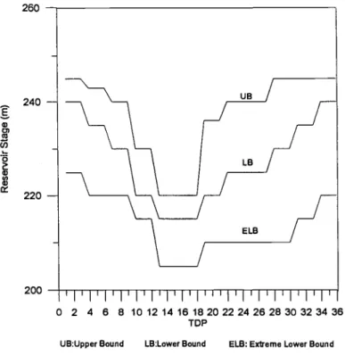
The operation of Shihmen Reservoir is based on a set of three rule curves, the upper bound, the lower
bound, and the extreme lower bound. Reservoir release is reduced from its normal release volume
when the reservoir stage falls below the lower bound of reservoir rule curves. Thus, from the perspective of reservoir operations, the onset of a drought can be defined as the time when reservoir stage falls below the lower bound of the rule curves. DLT can also be considered as the period of time during which normal
reservoir operations are maintained until the
approaching drought occurs.
During a drought, water rationing and water share reallocation for different established users are com-mon remedial measures. However, when and how to enforce these measures depends on knowing the DLT of an approaching drought. For example, cautionary measures such as prioritizing water users and reallo-cating their shares of water supply can be adopted for an impending drought. In this study, we not only com-pare two different approaches of drought prediction, but also assess their prediction accuracies.
METHODOLOGY
This section describes the procedures employed in
this study. These procedures include a reservoir
inflow prediction model, a regression model of reser-voir release prediction, and reserreser-voir mass balance analysis. These three major components, although
carried out in the same order as stated above, are
briefly introduced in the subsequent subsections in a reverse order to better demonstrate their association.
Reservoir Mass Balance Analysis
In Taiwan, a reservoir is operated on a
ten-day-period basis according to its rule curves and the water demands of the downstream users. The mass balance equation of the reservoir is:
S(t+1) =I(t+1)-R(t+1) ÷ S(t) (1)
where S(t) denotes the reservoir storage at the end of the tth period, I(t+1) represents the total inflow to the reservoir during the (t+1)thten-day-period,and R(t+1) is the total losses from the reservoir during the (t+1 )th ten-day-period including ground water seepage flow,
reservoir evaporation, and downstream water supply needs. To simplify the expression, the ten-day-period is abbreviated TDP hereafter.
Reservoir operation is briefly described as follows. At the end of the tth TDP, reservoir operation person-nel review the downstream water demands for the next TDP. The total release volume of the next TDP, R(t+1), and shares for different users are determined on the basis of the available storage in the reservoir S(t), the rule curve criterion, and reservoir manage-ment experiences. Thus, reservoir storage of the next TDP, S(t+1), can be predicted if the inflow I(t+1) is predicted, i.e.,
.(t+1) =I(t+1)-R(t+1) +S(t) (2) where (t+1) and I(t+1) are predicted values of S(t+1) and I(t+1), respectively. Reservoir stage of the next TDP, H(t+1), can then be determined with the assis-tance of the reservoir stage-storage relationship.
To extend the prediction even further, e.g., one
month, releases from the reservoir for the (t+2) and
(t+3) TDPs must also be predicted since reservoir
storages S(t+1) and S(t+2) are not known at time t.
Thus, the following equations are used to predict
reservoir storage one month in advance:
.(t+1) = I(t+1)-R(t+1) +S(t) (3a)
(t+2) =I(t÷2)-1t+2)+(t+1) (3b)
(t+3) =I(t+3)-t?(t+3) + .(t+2) (3c)
Notably, in Equation (3a), R(t+1) is the real reser-voir release of the (t+1) TDP, while in Equations (3b) and (3c), predicted releases R(t+2) and R(t+3) are used. Prediction of reservoir release is described later.
Reservoir In flow Prediction
Reservoir inflow is predicted using two different approaches: kriging method and time series analysis. The kriging method of estimation, also known as the theory of regionalized variables or geostatistics, was originally proposed to deal with spatially distributed data (Matheron, 1971). Discussions of kriging include Huijbregts and Matheron (1971), Matheron (1971, 1973), Journel (1974), Journel and Huijbregts (1978), Mantoglou and Wilson (1981), Myers (1982, 1984), and Kitanidis (1983). In addition, many hydrologists have applied kriging to solve problems such as moni-toring network design (Bastin et al., 1984; Virdee and Kottegoda, 1984; Kassim and Kottegoda, 1991), piezo-metric surface estimation (Rouhani, :1986; Rouhani
(Chua and Bras, 1982). Deihomme (1978) introduced geostatistical applications to the hydrosciences. We briefly introduce the most widely used ordinary krig-ing in this section.
Let Z(x) be a random variable at a spatial location x. We wish to estimate a value at x0 using data values observed at neighboring locations x1, i =1, 2, . . ., n,
and combine them linearly with weights X
(x0) = X1z(x).
The ordinary kriging assumes the following second-order stationary properties for the random field {Z(x),
xEQ}
E[Z(x)] 12z
Var[Z(x)] =
Cov[Z(x), Z(x)] =Cov( -
x
I)Vx E
l,
where 2 represents the domain of the studyarea. We require the kriging estimator to be unbiased and have minimum variance of estimation errors, i.e.,
E[Z(x0)] = E[Z(x0)]
minimizing Var[Z(x0) — Z(x0)].
Under these two constraints, we solve the following ordinary kriging system for A
i=1,2,...,n
=1 (lOb)
where ).1isa Lagrange multiplier and =y (I
x
-x
I) representsthe semi-variogram of the random fieldZ(x) and is defined as:
y(Ix
—xj I)=E{[Z(x)—Z(xi)]2} (11)Although kriging was initially proposed for dealing with spatially distributed data, Rouhani and Cargile (1989) applied universal kriging, which is a
Gaussian-Markovian interpolation method for nonstationary
random variables, to monthly reservoir inflow
(one-dimensional temporal data) prediction to yield an
estimate of DLT for a given reservoir operation policy
and initial conditions. In our study, the fact that
reservoir storage is predicted only for the dry season
accounts for why the mean of the random field is
assumed constant and ordinary kriging approach is adopted herein.
Let 1(t) represent total volume of reservoir inflow of the tth TDP. Future reservoir inflow I(tk) can be
esti-(4) mated by using n previously observed reservoir
inflows I(t), i =1,2,. . . , n.
I(t).
(12) (5) The weights Xjk being assigned to observed inflowscan be determined by solving the ordinary kriging (6) system of Equation (10) with Z(x) being replaced by
1(t). The semi-variogram characterizes the spatial (in
(7) our case, temporal) variability of the random field and must be established before solving the above system. Notably, Xjk are weights used for predicting reservoir inflow volume at time tk(k >n)and are dependent on the time at which a prediction is to be made.
Our time series approach of reservoir inflow
(8) prediction involves building an Autoregressive— Moving—Average (ARMA) model (Box et al., 1994) for
1(t). Prior to ARMA modeling, Fourier analysis is
per-(9) formed to determine the cyclic components embedded
in 1(t). If significant cyclic components exist, 1(t) is expressed as:
1(t) =C(t)+
(t)
(13)where C(t) denotes the cyclic component and (t)
rep-(lOa) resents the residual that will be modeled as an ARMA process. The cyclic component is the sum of several harmonic components and is expressed as:
NN
C(t) =a0+ ak cos(wkt) +I3pksin(o)kt) (14)
p=l k= 1
where N denotes the number of peaks in the
pen-odogram of 1(t), w are their angular frequencies, and N represents the number of harmonic components.
The ARMA(k,l) model of a stationary random pro-cess X(t) has the form of
k I
X(t) =
4X(t
—i)+e(t)+O(t
—j)
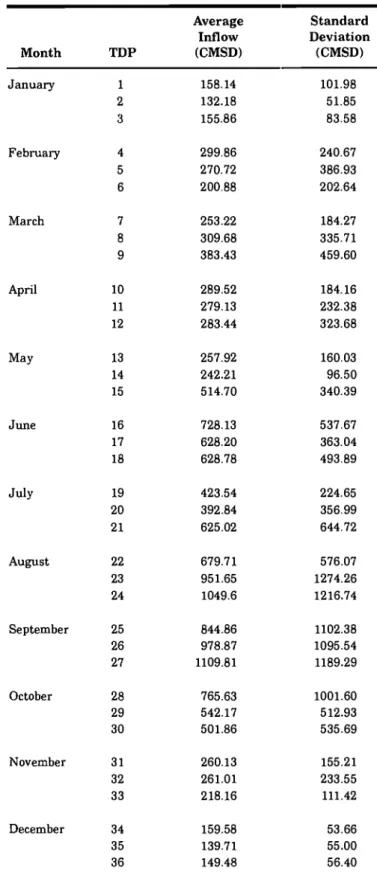
TABLE 1. Average and Standard Deviation of Ten-Day-Period Reservoir Inflow (1964-1993).
Average Standard Inflow Deviation Month TDP (CMSD) (CMSD) January 1 2 3 February 4 5 6 March 7 8 9 April 10 11 12 May 13 14 15 June 16 17 18 July 19 20 21 August 22 23 24 September 25 26 27 October 28 29 30 November 31 32 33 December 34 35 36
where c(t) are white noise with zero mean and vari-ance cyL and 's and Os's are the autoregressive and moving average parameters, respectively. If 0, =0 for
j
= 1,2,. .. 1,we say that we have an autoregressive orAR(k) model, whereas if 4= 0 for i =1,2, . . . ,k, we
have a moving average or MA(l) model. The readers are referred to Priestley (1981) and Shih and Cheng (1989) for detailed description of the modeling. As assumed herein, polynomial trend does not exist in
Reservoir Release Prediction
As mentioned earlier, reservoir release of the next TDP, i.e., R(t+1), is determined at the end of the cur-rent TDP based on the available reservoir storage and
management experiences. In general, reservoir
release is reduced from its normal release volume of the corresponding TDP once the reservoir stage falls below the lower bound of the rule curves. Thus, it is reasonable to predict R(t+2) and R(t+3) based on aregression equation of reservoir stage H(t) versus
reservoir release R(t+1). A set of TDP-speciflc regres-sion relationships of H(t) versus R(t+1) is established for H(t) which is below the lower bound. From Equa-tion (3a), (t+1) can be predicted, and then, H(t+1) can
be calculated using the stage-storage relationship.
R(t+2) is thus calculated using the regression equa-tion of H(t) versus R(t+1) if H(t+1) is found below the lower bound of the rule curve. If H(t+1) exceeds the lower bound, then the normal release volume should apply. 1t+3) can also be calculated in a similar man-ner.
CASE STUDY
The Shihmen Reservoir, located in northern Tai-wan, with a drainage basin of 763 kin2, was selected as our study site. Thirty years (1964-1993) of the
ten-day-period reservoir inflow data were used in this study. As Table 1 illustrates, inflow data reveal a
strong seasonal variation. The dry season runs from November 1 (beginning of the 31st TDP) to May 20 (end of the 14th TDP) of the next year. Figure 1 dis-plays the reservoir operation rule curves.
Kriging Approach to Reservoir Inflow Prediction
For the kriging approach to reservoir inflow
prediction, structural analysis was initially performed to yield a variogram that characterizes the temporal158.14 132.18 155.86 299.86 270.72 200.88 253.22 309.68 383.43 289.52 279.13 283.44 257.92 242.21 514.70 728.13 628.20 628.78 423.54 392.84 625.02 679.71 951.65 1049.6 844.86 978.87 1109.81 765.63 542.17 501.86 260.13 261.01 218.16 159.58 139.71 149.48 101.98 51.85 83.58 240.67 386.93 202.64 184.27 335.71 459.60 184.16 232.38 323.68 160.03 96.50 340.39 537.67 363.04 493.89 224.65 356.99 644.72 576.07 1274.26 1216.74 1102.38 1095.54 1189.29 1001.60 512.93 535.69 155.21 233.55 111.42 53.66 55.00 56.40
variation of 1(t). In our study, the inflow variogram was estimated using dry season reservoir inflow data. From the 30 years of inflow data, we first calculated experimental variograms for each of the 29 dry sea-sons. Next, the following exponential model (Figure 2), which characterizes the temporal variation of dry season reservoir inflows, was fitted to the average of the 29 dry-season inflow variograms:
y(h) = 62600 [1-exp(-h/2.35)1 (16)
Here y(h) denotes the variogram in (cms-day)2 and h represents the time interval in TDP.
260 240 E a, a, Ca (I, 220 200 o 2 4 6 8 1012141618202224262630323436 TOP
UB:Upper Bound LB:Lower Bound ELB: Exeme Lower Bound
Figure 1. Operation Rule Curves of Shilimen Reservoir.
In Equation (12), previous observations 1(t1), i =1,
2, . . . n,are needed to predict I(tk). Herein, we use three consecutive observations (n =3) to predict the
next three inflows. Thus, the first predicted reservoir inflow was that of December 1 through December 10 (the fourth TDP of each dry season). Use of more pre-viously observed data would lag our first prediction since the first prediction must be lagged n TDPs from the beginning of the dry season. For instance, if five previous observations (n = 5) were used, reservoir
inflow of December 21 through Deèember 31 would be the first predicted reservoir inflow.
The kriging weights 2 can be obtained from
Equa-tion (10) without knowing any real measurements since the variogram is only a function of distance.
Therefore, reservoir inflow volumes of the immediate next three TDPs do not need to be predicted in their
temporal order since Y,j in Equation (lOa) depends only on points of observations used for prediction (ti, i =1,2,. . . ,n)and the time at which prediction is to be made (tk). Except the first two TDPs of each dry sea-son, there are three predictions of reservoir inflows
for each TDP. x 10000) 8 2 0 $ 4 8 12 18 20 h(10DAYS))
Figure 2. Variogram of the Dry Season Reservoir Inflow.
Time Series Approach to Reservoir In flow Prediction In contrast with the kriging approach for which
predictions of reservoir inflows are based on the
dry-season variogram only, the time series approach
requires consecutive all-season inflow data for ARMA model building. In this study, we analyzed ten-day-period reservoir inflows from 1964 to 1993. Fourier analysis of the reservoir inflow data revealed two sig-nificant frequencies, Wi = 0.17453and W2 = 0.47124
(Figure 3). Corresponding periods of the two frequen-cies are 36 TDPs and 13 TDPs, strongly reflecting the
annual cycle and seasonal variations of reservoir inflows. The harmonic components embedded in
reservoir inflow were identified as:
C(t) =a0+a11cos W1t + f3 sin w1t + a12 cos2 w1t
+ /12sin2 w1t + $13 sin3 w1t +$14sin4 w1t
+ /3sin6 W1t + $21 sinw2t
where a0 =444.43,a11 = -216.56,f11 =-241.22, a12 = -130.54,/312 83.77, $i = 88.88, $14 = -75.98, $16 =
-55.47,
and f
= 61.90.The residual c(t) is identified as an AR(1) process
based on its partial autocorrelation function and
(t) = 0.36175(t-1) +E(t)
where (c(t)} is a purely random process with zero
mean, and variance o= 42,127 (cms-day)2. Similar to the kriging approach, three predictions can be made for each TDP. However, time series approach of reser-voir inflow prediction for the next three consecutive TDPs must be carried out in their temporal order.
60
Simulation of Reservoir Operation
The stage-storage relationship of Shihmen reser-voir is expressed by the following equation:
S =0.0174(H -158.3)2.71 (19)
where S denotes the reservoir storage volume in ems-day (CMSD), and H represents the reservoir stage in meters above the mean sea level.
Two drought conditions are defined. Moderate
drought occurs when reservoir stage falls between the lower bound and the extreme lower bound of the rule curves. Extreme drought occurs when the reservoir stage is below the extreme lower bound. The reservoir operation was simulated for each of the 29 dry sea-sons. As mentioned earlier, release volumes R(t+2) and R(t+3) must be predicted prior to predicting the
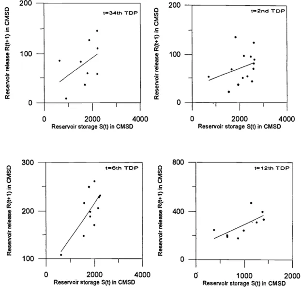
(18) reservoir storages S(t+2) and S(t+3). In general, reser-voir release is reduced from its normal release volume of the corresponding TDP once the reservoir stage falls below the lower bound of the rule curves. If the reservoir stage exceeds the lower bound, downstream water demands are usually fully provided. Figure 4 provides examples of the S(t)-.R(t+1) relation for S(t) lower than the lower bound. Since h:istoric records
were used for simulation, whenever the predicted
drought/no-drought condition was cons:istent with the historic condition, the historic release volume of the next TDP, R(t+1), was adopted. Two types of release
volume predictions may apply if our simulations result in conflict drought/no-drought conditions against historic records. Initially, if a drought was
predicted while no drought actually occurred, then release volume of the next TDP was predicted using regression equation of S(t) versus R(t+1) with S(t)
being lower than the lower bound. Second, if no
drought was predicted while a drought did occur, then R(t+1) was predicted using regression equation of S(t) versus R(t+1) with S(t) being higher than the lower
bound.
An indicator of an approaching drought, i.e., the drought lead time, was determined as DLT = k if a
drought was predicted to occur k TDPs later. In our study, DLT 3 since only S(t+1), S(t+2), and S(t+3) are predicted.
Evaluating Probability of Success of Drought Prediction
As mentioned earlier, three predictions of reservoir stage can be made for each TDP (except for the first two) in the dry period; each of these predictions
corre-sponds to drought lead time of 1, 2,, and 3 TDPs,
respectively. According to results obtained from 29 dry-season simulations, the probability of success (Ps) of drought prediction, defined as the ratio of number of correct predictions to total number of predictions,
for each TDP was tabulated in Tables 2 and 3.
Drought prediction using kriging approach to reser-voir inflow prediction clearly has a higher Ps than using the time series approach for both. moderate and severe drought conditions. For moderate droughtcon-ditions, at lead time of three TDPs, the kriging
approach generally has a Ps exceeding 0.8 (except for the 9th, 10th, and 12th TDPs) with an average of 0.86,while the average Ps is 0.78 for the time series
approach. Especially in the period between the 5thand the 8th TDPs, the kriging approach performs
much better than the time series approach. The supe-riority of the kriging approach in this period is signifi-cant in that during this period an enormous amount 0
40-
(I)0
E a) 0 0 20-0— = 0.17453 0)2 = 0.47124 0 1 2 3 Freguency,wFigure 4. S(t)—R(t+1) Relationship for S(t) Lower Than the Storage of the Lower Bound of Reservoir Rule Curves.
of water is supplied to irrigate rice paddies.
Accurate-iy predicting the occurrence of the approaching
drought in this period would facilitate watermanage-ment authorities in reaching better decisions. For severe drought conditions, at a lead time of three
TDPs, the kriging approach has an average Ps of 0.93 compared to 0.92 for the time series approach. The probability of success is critical in that it can be used by the reservoir agency to determine whether, at any TDP, remedial actions should be taken in response to a predicted future drought. For instance, a reservoir agency may decide to take remedial actions only if the Ps of that TDP exceeds 0.80. Thus, for a moderate
drought, the kriging approach would require taking actions for most TDPs except the lOth, and l2th
TDPs if drought is predicted one month in advance. However, the time series approach requires adopting actions for only the 34th, 35th, 3rd, 4th, 10th, and 11th TDPs under the same circumstance.
An example of potential management practice using the information of DLT and Ps is described below.
If, at the end of March (end of the 9th TDP), as pre-dicted, a moderate drought will occur at the end of April (DLT = 3), no remedial actions are taken since
Ps of the 12th TDP, Ps(12), is 0.76 (lower than 0.80) for both approaches. However, if a severe drought is predicted to occur one month later, minor remedial actions are taken since Ps(12) is 0.97 and 0.90 for the kriging and time series approaches, respectively. As time passes, at the end of the lOth TDP, an approach-ing moderate drought is predicted to occur at the end of April, so moderate remedy actions are taken since Ps(12) =0.86 > 0.80and DLT =2only. Finally, at the end of the 11th TDP, a moderate drought is predicted to occur one TDP later (DLT=1) and Ps(12) = 0.97, so major remedy actions will be taken. The reservoir
agency may take different levels of remedy actions:
c
C) t34th TOP0
200— t2nd TDP.
- ..
-,—.
a, a,.
•3 a).
.
0.
a,a 100—,/,zv
a,.
• a) • 0 I I.
S S 100— S • • 0.
I 0 2000 4000 Reservoirstorage S(t) in CMSD 0 2000 4000 Reservoirstorage S(t) in CMSD (I, 300— — t—eth TDP 0-12th TOP 0 •.
- S .I
a)i
.5 200— -— . ••(
•
a,a
• 100— I I 0 2000 4000 Reservoirstorage S(t) in CMSD I I 0' 1000 2000 Reservoirstorage S(t) in CMSD 800 Co 0 C + a, a, 0 a, 400 I 0TABLE 2. Probability of Success of Drought Prediction (Ps) (kr.iging approach of inflow prediction).
DLT =3 TDPs DLT =2 TDPs DLT =
Moderate Severe Moderate Severe Moderate 1 TDPSevere
t Drought Drought Drought Drought Drought Drought
34 0.90 1.00 35 0.97 1.00 1.00 1.00 36 0.90 0.97 0.97 0.97 1.00 0.97 1 0.90 0.97 0.97 0.97 0.93 1.00 2 0.86 0.97 0.90 1.00 0.97 1.00 3 0.86 1.00 0.90 1.00 0.97 1.00 4 0.86 1.00 0.97 1.00 0.90 1.00 5 0.90 0.93 0.83 0.93 0.90 1.00 6 0.86 0.90 0.93 0.97 1.00 1.00 7 0.86 0.97 1.00 1.00 0.97 1.00 8 0.83 0.93 0.93 1.00 0.97 1.00 9 0.72 0.86 0.79 0.90 0.90 1.00 10 0.79 0.86 0.90 1.00 0.97 1.00 11 0.86 0.90 0.79 1.00 1.00 0.97 12 0.76 0.97 0.86 0.93 0.97 1.00 13 0.83 0.86 0.93 0.93 0.97 0.97 14 0.93 0.90 0.93 0.93 0.97 1.00 Average 0.86 0.94 0.91 0.97 0.96 0.99
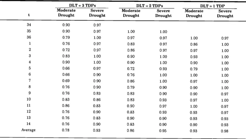
TABLE 3. Probability of Success of Drought Prediction (Ps) (time series approach of inflow prediction).
DLT=3TDPs DLT=2TDPs DLT=LTDP
Moderate Severe Moderate Severe Moderate Severe
t Drought Drought Drought Drought Drought Drought
34 0.90 0.97 35 0.90 0.97 1.00 1.00 36 0.79 1.00 0.97 0.97 1.00 0.97 1 0.76 0.97 0.83 0.97 0.86 1.00 2 0.72 0.97 0.86 0.97 0.97 1.00 3 0.83 1.00 0.90 1.00 0.93 1.00 4 0.90 1.00 0.90 1.00 0.90 1.00 5 0.66 0.97 0.72 0.93 0.79 1.00 6 0.66 0.90 0.76 1.00 1.00 1.00 7 0.69 0.90 0.86 1.00 0.97 1.00 8 0.76 0.90 0.79 0.90 0.90 1.00 9 0.76 0.83 0.83 0.90 0.90 0.97 10 0.83 0.86 0.83 0.93 0.97 1.00 11 0.86 0.83 0.90 0.97 1.00 0.97 12 0.76 0.90 0.83 0.93 0.93 0.97 13 0.76 0.83 0.90 0.90 0.93 0.93 14 0.76 0.90 0.83 0.90 0.90 0.93 Average 0.78 0.93 0.86 0.95 0.93 0.98
minor, moderate, or major actions according to the drought lead time. For a severe drought, similar man-agement practice may apply but with higher Ps, e.g.,
0.90.
Estimated DLT of Historical Drought Events
The above discussions have concentrated on pre-dicting the drought occurrence for specific TDPs and the probability of success of drought prediction for each TDP. We now turn our attention to the DLT of each historical drought event, which normally lasts for several TDPs. During the drought run length, pre-diction of droughtino-drought occurrence can be made for each TDP, and thus, several predictions of drought occurrence can be made during a drought run. Herein, we focus merely on evaluating the lead time at which onset of historical droughts were correctly predicted.
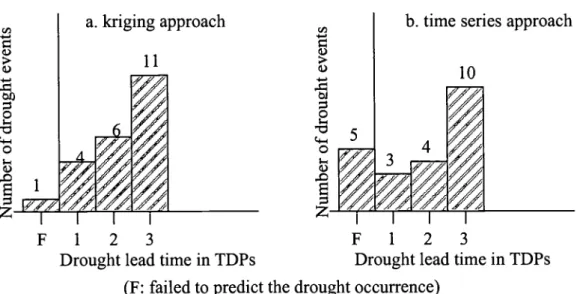
From 1964 to 1993, there were 22 moderate
drought events and nine severe drought events. The onset of these events was correctly predicted by thekriging and time series approaches with various
DLTs, as shown in Figures 5 and 6. For the kriging approach, approximately 77 percent of total moderate drought events were correctly predicted at least two TDPs in advance (DLT 2) and only one event failed to be predicted. For the time series approach, only 64 percent of moderate drought events were correctly
predicted at least two TDPs in advance and five events (23 percent) were not predicted at all. For
severe drought events, approximately 78 percent were correctly predicted at least two TDPs in advance by
5)
0
0
the kriging approach with no failed event; however, only 11 percent of severe drought events were correct-ly predicted at least two TDPs in advance by the time series approach, and 22 percent of events failed to be predicted. The kriging approach clearly outperformed
the time series approach in terms of the number of drought events being correctly predicted and their DLTs.
Duration and Water Deficit of Droughts
The severity of a drought event is usually described by its duration and water deficit. The duration, or the run length, is defined as the time span of a drought event. In this study, we define the water deficit as the departure of reservoir storage from its normal
vol-ume. Other applications also use precipitation or
stream flow to characterize the water deficit.
Since both the kriging and time series approaches make drought predictions with lead time less than or equal to three TDPs, they do not provide information about the drought duration for events lasting longer
than three TDPs. As for the water deficit, both
approaches predict reservoir storages for the next three TDPs, and thus, future water deficits can be
estimated. —
Let D(t) and S(t) be the water deficit and normal reservoir storage of the tth TDP, respectively. Based on our definition for water deficit and Equation (1), the predicted water deficit is
a. kriging approach
/
b. time series approach
10 5) 5) 0 0 I I I I F
123
Drought lead time in TDPs
F 123
Drought lead time in TDPs (F: failed to predict the drought occurrence)Figure 5. Successful Drought Prediction for Various DLTs for Moderate Drought Events: (a) Kriging Approach and (b) Time Series Approach.
V -c 0 0 I-V
-
EF 123
Drought lead time in TDPs123
Drought lead time in TDPs
Figure 6. Successful Drought Prediction for Various DLTs for Severe Drought Events: (a) Kriging Approach and (b) Time Series Approach.
D(t+1)=S(t)—(t+1)
D(t+ 1) = S(t) — S(t +1)+1(t+ 1)—R(t+ 1)
where S(t) =
S(t),
and S(t)is the tth TDP reser-voir storage of the th year. Clearly, predicting thereservoir storage S(t+1) is equivalent to predicting the
water deficit D(t+1).
Under current reservoir operations, reservoir
release of the next TDP, i.e., R(t+1), is determined based on the available reservoir storage S(t) and the management experiences of the operation personnel. In this study, we established regression relations for reservoir storage S(t) and reservoir release volume R(t+1) to simulate the current practice of reservoir operations. This decision making process does not involve the potential water deficit. However, it is pos-sible to use R(t÷1) estimated by the current practice as an initial estimate, and then iteratively fine-tuneR(t+1) by examining the predicted water deficit
D(t+1). In that case, regression equations for S(t) and R(t+1) only provide an initial estimate for R(t+1), and the management experiences of the operation person-nel will play a more important role in determining the final R(t+1). However, equations for reservoir balance
analysis (Equations 3a, 3b, and 3c) and reservoir
inflow prediction (Equations 12 and 13) should still be used for drought forecasting. Improvement in
reser-voir operations is likely by considering potential
water deficit in the decision-making process.
(20) CONCLUSIONS
An indicator of an approaching drought is
particu-(21) larly important for reservoir operations in Taiwan.
The indicator signals the onset of approaching
drought and can be used by reservoir management authorities to decide whether, when, and whatreme-dial measures should be adopted. In this study the
drought lead time was used as an indicator for
drought management. Drought predict.ions wereper-formed using approaches of the kriging and time
series analysis and a subsequent reservoir operation simulation. According to simulation results, the
krig-ing approach is clearly better than the time series
approach in terms of the number of droughts being correctly predicted, the DLTs, and the probability of success of drought prediction. The superiority of the kriging approach may partially be att.ributed to the fact that reservoir inflow variogram is established
using only dry-season reservoir inflows and more
accurately represents the temporal variation of reser-voir inflow of that particular season. ]:n comparison, the time series approach must use all available and consecutive reservoir inflows to develop an ARMA model. Thus, the ARMA model considers the temporal variation of the entire process, dry- and wet-season both included. After removing the cyclic components,
the temporal variation characteristics of reservoir
inflow in dry-season and wet-season are assumed the
same in the time series approach. The kriging
approach is also advantageous in that it does not require using continuous and regularly sampled
inflow data. This feature makes it more applicable when missing data are encountered in the time series. a. kriging approach b. time series approach
4
0 - '.4-0 6 1Using the information of drought lead time and
probability of success of drought prediction, reservoir
operation in the dry season can be more efficient. However, reservoir management authorities must
determine what probability of success is required to prompt taking remedial measures for moderate and severe droughts, e.g., 0.8 and 0.9, respectively. Also, different levels (minor, moderate, and major) of reme-dial measures should be planned and adopted accord-ing to the length of the predicted drought lead time.
ACKNOWLEDGMENTS
We gratefully acknowledge the National Science Council of the
Republic of China for financially supporting this research.
Dr. Rouhani of the Georgia Institute of Thchnology is also appreci-ated for providing valuable reference works. We also acknowledge valuable comments by anonymous reviewers.
LITERATURE CITED
Bastin, G., B. Lorent, C. Duque, and M. Gevers, 1984. Optimal Estimation of the Average Areal Rainfall and Optimal Selection of Raingauge Locations. Water Resources Research 20(4):463-470.
Bonacci, 0., 1993. Hydrological Identification of Drought. Hydrolog-ical Processes 7:249-262.
Box, G. E. P., G. M. Jenkins, and G. C. Reinsel, 1994. Time Series Analysis: Forecasting and Control. Prectice-Hall, London,
Unit-ed Kingdom, 598 pp.
Chua, S. H. and R. L. Bras, 1982. Optimal Estimation of Mean Areal Precipitation in Regions of Orographic Influence. Journal of Hydrology 57:713-728.
Delhomme, J. P., 1978. Kriging in Hydrosciences. Advances in Water Resources 1(5):251-266.
Huijbregts, C. J. and G. Matheron, 1971. Universal Kriging: An Optimal Method for Estimating and Contouring in Trend Sur-face Analysis. In: Proceedings of Ninth International Sympo-sium on Techniques for Decision-Making in the Mineral Industry, J. I. McGerrigle (Editor). The Canadian Institute of Mining and Metallurgy Special Volume 12, pp. 159-169.
Journel, A. G., 1974. Geostatistics for Conditional Simulation of Ore Bodies. Economic Geology 69:673-687.
Journel, A. G. and Ch. J. Huijbregts, 1978. Mining Geostatistics. Academic Press, New York, New York, 600 pp.
Kassim, A. H. M. and N. T. Kottegoda, 1991. Rainfall Network Design Through Comparative Kriging Methods. Hydrological Sciences Journal 36(3):223-240.
Kitanidis, P. K., 1983. Statistical Estimation of Polynomial Gener-alized Covariance Function and Hydrological Applications. Water Resources Research 19(4):909-921.
Mantoglou, A. and J. L. Wilson, 1981. The Turning Bands Method for Simulation of Random Fields Using Linear Generation by a Spectral Method. Water Resources Research 18(5):1379-1394. Matheron, G., 1971. The Theory of Regionalized Variables and Its
Applications. Les Cahiers du Centre de Morphologie Mathema-tique, No, 5. Centre de GeostatisMathema-tique, Fontainemlea, France. Matheron, G., 1973. The Intrinsic Random Functions and Their
Applications. Advances in Applied Probability 5:439-468. Myers, D. E., 1982. Matrix Formulation of Cokriging. Mathematical
Geology 14: 249-257.
Myers, D. E., 1984. Cokriging: New Developments. In: Geostatistics for Natural Resource Characterization, G. Verly et al. (Editors). D. Reidel, Dordrecht, Germany, pp. 295-305.
Priestley, M. B., 1981. Spectral Analysis and Time Series. Academic Press, London, United Kingdom, 890 pp.
Rossi, G., M. Benedini, G. Tsakiris, and S. Giakoumakis, 1992. On Regional Drought Estimation and Analysis. Water Resources Management 6:249-277.
Rouhani, S., 1986. Comparative Study of Groundwater Mapping Thchniques. Journal of Ground Water 24:207-216.
Rouhani, S. and K. A. Cargile, 1989. A Geostatistical Tool for Drought Management. Journal of Hydrology 108:257-266. Rouhani, S. and T. J. Hall, 1989. Space-Time Kriging of
Ground-water Data. In: Geostatistics, M. Armstrong (Editor). Kiuwer Academic Publishers, Vol. 2, pp. 639-651.
Shih, S. F. and K. S. Cheng, 1989. Generation of Synthetic and Missing Climatic Data for Puerto Rico. Water Resources Bul-letin 25(4):829-836.
Virdee, T. S. and N. T. Kottegoda, 1984. A Brief Review of Kriging and Its Application to Optimal Interpolation and Observation Well Selection. Hydrological Sciences Journal 29(4):367-387.