MODELING THE SUPPLY-DEMAND INTERACTION IN ELECTRONIC
COMMERCE: A BI-LEVEL PROGRAMMING APPROACH
Daniel Y. Shee
Department of Management Information Systems National Chengchi University, Taipei, Taiwan
daniel@mis.nccu.edu.tw
Tzung-I Tang
Department of Management Information Systems National Chengchi University, Taipei, Taiwan
mtang@nccu.edu.tw
Gwo-Hshiung Tzeng Institute of Technology Management National Chiao Tung University, Hsinchu, Taiwan
ghtzeng@cc.nctu.edu.tw
ABSTRACT
The purpose of this paper consists in establishing the model for the supply-demand interaction in the age of electronic commerce. First of all, the study uses the individual objectives of both parties as the foundation of the supply-demand interaction. Subsequently, it divides the interaction, in the age of electronic commerce, into the following two classifications: (i) Market transactions, with the primary focus on the supply-demand relationship in the marketplace; and (ii) Information service, with the primary focus on the provider and the user of information service. This study focusing on the proceeding two classifications, and in accordance with the relationship types and dominance, will proceed to divide the supply-demand relationship into four parts for discussion. By applying the bi-level programming technique and a flow chart of interaction process, the study will develop an analytical process to explain how supply-demand interaction achieves a compromise or why the process fails. Finally, it will provide an example of information service for explaining bi-level programming technique’s practical applied process.
Keywords: Electronic commerce, Supply-demand interaction, Information service provider, Bi-level programming
1. Introduction
Under constant pressure from changing global marketing trends, traditional relationships in supply and demand have necessarily gone through a number of radical changes. In the past ten years alone, information technology (IT), whilst consistently producing performance enhancement, has also brought about a corresponding rapid decline in costs. This, combined with the continuing expansion of global communications networks, has allowed the major players of markets to create extensive and sustainable competitive advantage [Cash & Konsynski, 1985; Porter & Millar, 1985; Bakos, 1991a; Kekre & Mudhopadhyay, 1992]. The proliferation of the IT and communication networks also provided the framework upon which electronic commerce (EC) -- an amalgamation of many different processes, technologies, applications and business strategies that are fundamental to electronic business [Taylor & Berg, 1995] -- could subsequently develop. It now provides the base from which companies are able to coordinate their everyday transactions with their business partners, with the end result that these increasingly effective and efficient business management processes create the need to constantly redefine traditional supply-demand relationships.
With EC performing so well in the coordination of buyers and suppliers, many scholars have felt the need to research this area; industry is also embracing EC to improve industrial relations [Roberts & Mackay, 1998; Tang et al., 1999; Tang et al., 2000]. Amongst the many prevalent issues created by the introduction of EC systems is the ease with which flexible and adaptable structures in the supply-demand relationship can be established to provide the driving force for cooperation through strategic alliances between trading parties [Roberts & Mackay, 1998]. The key issue, therefore, is how the demanders and suppliers facilitate this interaction.
In this paper, aspects of supply-demand interaction in the EC environment are analyzed. Firstly, the paper examines the EC environment and its characteristics, continuing with a discussion on supply chain management (SCM) and an exploration of the impact of EC on SCM. Secondly, based on the conceptual model proposed by
Tang et al. [1999], our analysis will be conducted on the following two kinds of supply-demand interaction: (i) the buyer-supplier interaction occurring in the market transaction and (ii) the interaction between the user and provider of the information services. Thirdly, the bi-level programming technique will be utilized to model the aforementioned interactions and an example will be used as an illustration. Finally, this paper provides some discussions and conclusions derived from the study.
2. EC and SCM
The framework of EC and its inherent methods can be applied to a wide range of domains. It has great potential to facilitate the coordination of the supply-demand relationship in a supply chain. In this section, from the viewpoint of the attributes of EC, we will discuss the nature of SCM and the impacts of EC on SCM.
2.1. The Attributes of EC
The use of IT, characterized by high performance at reduced cost, is widespread, and in tandem with the maturity in both bandwidth and reliability of global communications infrastructure has created the emergence of “new generation business” which radically changes traditional business methods [Wigand & Benjamin, 1995]. EC, a relatively new phenomenon, comprises unique features that distinguish it from traditional commercial models and, in recent years, it has been applied to a growing range of industries, including interactive home shopping [Rowley, 1996; Alba et al., 1997], travel [Bloch & Segev, 1997], health care [Barbaro, 1996], supply chain management [Hinkkanen et al., 1997; Roberts & Mackay, 1998] and even the not-for-profit fields of education and digital libraries [Adam et al., 1996].
The start point in characterizing EC is the medium used. Examples of this are the tools used by companies such as electronic data interchange (EDI) and email, which provide paper-free, electronic business connections [Kekre & Mudhopadhyay, 1992]; and the Internet and its applications (e.g. the World Wide Web), which are seen as the new-wave media [Wigand, 1995; Hoffman & Novak, 1996].
Furthermore, transactions in the world of EC are no longer limited to traditional goods. In comparison to tangible goods (such as clothes, books, etc), that have to be sent through physical distribution channels, the more intangible services and information are electronically passed through interconnected networks that enhance the content of EC. This provision of both tangible and intangible goods has, therefore, widened the range of transactions, and increased the number of companies using EC to conduct business.
Transactions undertaken in EC usually involve three main parties: (i) the buyer; (ii) the supplier; and (iii) the information service provider (ISP). The ISP acts as an intermediary providing a broad range of services such as: EDI, email delivery, file transfer and electronic fund transfers [Tallarico, 1998]. The mediating role of the ISP in EC is echoed by Bakos [1991a, 1991b], who sees them as operating electronic market systems either as a market participant, an independent third party or a multi-firm consortium.
2.2. Supply Chain Management and the Impact of EC
The term “supply chain management (SCM)” seems to have originated in the early 1980s to describe the potential benefits of integrating internal business purchase, manufacturing, sale and distribution functions [Harland, 1996]. SCM provides the means for organizations to integrate planning and control of the processes and functions performed inside the industrial network from procurement, manufacturing and production through distribution. Previously, businesses had concentrated their attention on effective decision-making within the company. Today, however, increasing customer expectations and global competition demand that business moves away from maintaining their limited range of strategic advantages and expand their ability to compete simultaneously on quality, price, delivery lead time and reliability [Scott & Westbrook, 1991; Ellram, 1991; Harland et al., 1993; Harland, 1996; Thomas & Griffin, 1996].
A number of studies have concentrated on this area since the 1980s, and have defined SCM from different perspectives. Ellram’s [1991] broad perspective looked at industrial organization theory, transaction cost analysis and competitive strategy as the theoretical roots of modern SCM research. Harland et al. [1993] based their research on the management of processes, the process/service package, and supply chain resources, which together were designed to satisfy the combined needs of the end consumer. Lambert et al. [1998] pointed out that SCM is the integration of key business process from end customer through original suppliers that provides products, services, and information that add value for customers and other stakeholders. Mabert & Venkataramanan [1998] defined supply chain as the network of facilities and activities that performs the functions of product development, procurement, manufacturing, distribution, and after-market support for sustainment. According to these viewpoints, the objectives of SCM can be determined as coordinating and optimizing functions of supply-demand relationships that manage the flows of products/services and information that carries control and feedback mechanisms. In other words, SCM aims to provide advantages in customer satisfaction, cost reduction, quality improvement and flexibility enhancement [Jenkins & Wright, 1998].
The Value Chain Model, a well-known analytic framework developed by Porter [1985], considers the principal activities, which are present in the link from supplier to demander, and takes IT as a key element in facilitating the performance of these activities. In the EC environment, IT allows closer integration of adjoining steps on the value-added chain through the development of electronic markets and electronic hierarchies [Malone et al., 1987]. Advancements in electronic interconnection have greatly reduced costs and the time involved in information exchange by tightly linking the process from supplier to buyer and helping them to search, filter, and match parties relative to each transaction much more effectively. Malone et al. [1987] identified these as the “electronic interconnection effects”.
From another perspective, based on the relationship between suppliers and customers in a vertical market, it is claimed that the initiation of electronic market systems can have two possible outcomes: (i) an increase in competition, and (ii) a reduction in the supplier’s power [Bakos, 1991a; 1991b]. This suggests that buyers and suppliers can benefit from each other. With a wide choice of suppliers available for buyers to make their purchasing choices, buyers are benefited with products available at lower prices and suppliers can charge for the market information that they provide [Bakos, 1991a; 1991b; Wigand & Benjamin, 1995]. As Malone et al. [1987] suggest, the effects brought to market by the electronic market system stimulate the evolution of the market from a biased environment, to a market which is both unbiased and personalized.
3. Analyzing Different Supply-Demand Interactions
In this section, the discussion will focus on different supply-demand interactions existing in the EC environment. Starting with the interaction occurring in the transacting market, the rationale of the buyer-supplier interaction with intermediary’s (or cybermediary’s) mediation will be demonstrated. This will be followed by a discussion about the relationship between the user and provider of the information service; the role of the ISP as a mediator is analyzed.
3.1. The Buyer-supplier Interaction with ISP’s Mediation
Tang et al., [1999] have proposed a conceptual model to explore the interactive nature of the buyer-supplier relationship in the era of EC. By taking ISP as an intermediary their model includes the buyer, supplier and ISP as three major parties, and focuses on the electronic market dealing with the relationship level and the bilateral relationship mediated by the ISP. They conclude that the rationale of interaction between buyer and supplier is rooted in individual party’s objectives which usually fall into two categories: cost and quality. This model also takes the following three items into consideration: (i) information flow; (ii) flow of goods or services; and (iii) feedback information, as shown in Figure 1.
Information Service Provider
Buyer Supplier
Information
Flow InformationFlow
Goods or Service Flow Feedback Information Min [Cost]
Max [Quality of Information Service]
Min [Cost]
Max [Quality of Customer Service]
Min [Cost]
Max [Quality of Production & Manufacturing] Max [Quality of Distribution]
A specific supply-demand relationship inside a SC (EC Application Provider)
Figure 1: Interactive buyer-supplier relationship with ISP’s mediation [Source: Tang et al., 1999]
This conceptual model generalized the preliminary form of the supply-demand interaction with ISP’s mediation inside a specific supply chain. Obviously, there are two kinds of bilateral interaction, which are embedded in the model and are deserving of further analysis [Tang et al., 2000]. They are (i) the interaction between buyer and supplier and (ii) the interaction between the user (supply chain) and provider of the information service (or EC applications). For the latter, in particular, the “user” refers to both the buyer and supplier by taking them as a single party, whilst the term “providers” relates to the ISP industry.
In the past, several researchers have sought deeper insight into the rationale of supply-demand interactions. The various forms that supply-demand interactions can take often cause problems and make analysis somewhat difficult. Since Harland [1996] came to the conclusion that SCM can take place at different levels of relationships, chains and networks by taking a systematic approach in analyzing research and conceptual development of the SCM, there has been a wide acceptance by academics, consultants and operational
management of the fact that the type of relationship greatly contributes to the shaping of supply chain structure, and influences the methods with which business parties interact with one another [Groves & Valsamakis, 1998; Carter et al., 1998]. Adversarial and collaborative are two primary relationship categories often referred to in traditional buyer-supplier relationships that characterize such relationships [Lamming, 1986; Lyon et al., 1990; Imrie & Morris, 1992; Macbeth & Ferguson, 1994; Matthyssens & Van den Bulte, 1994]. Relevant researches on the aforementioned characterization discover the development of many new forms of this relationship, such as: long-term contracts, joint ventures, partnership sourcing and reduction and consolidation of the supply base [Imrie & Morris, 1992; Macbeth & Ferguson, 1994; Matthyssens & Van den Bulte, 1994]. Definitions of these new forms of the relationship were made with the purpose of integrating key processes, and interlocking the systems of quality, stocking and delivery.
On the other hand, additional factors that influence the interaction between transactional parties include the question of which company dominates in the relationship and to what extent the domination stands. For instance, a supplier’s chance for independent development is hindered in the buyer-dominated markets, and a dominating buyer often starts the supply chain and has controls over the production development and the end product [Brege et al., 1993; Lilliecreutz, 1998]. Within a relationship where the dominance cannot reach a balance, asymmetry in dependence, knowledge, initiation of change, etc can happen [Holmlund & Kock, 1996]. In such relationships, the dominators often anticipate their transactional partners to follow their strategies adoption [Lilliecreutz, 1998], and the non-dominators are expected to act like voluntary parties [Astley & Van de Ven, 1983]. Hence, the dominance in a relationship can lead to a difference in interaction between buyers and suppliers. Collaborative Adversarial Demander Supplier Quadrant I Quadrant II Quadrant IV Quadrant III
Horizontal Axis: Type of Relationship
Vertical Axis: The Dominator of the Relationship
Figure 2: The classification of supply-demand interaction [Source: Tang et al., 2000]
Tang et al. [2000], based on the dichotomy of the type of relationship, in association with the nature of unbalanced dominance within a relationship, suggested a classification scheme, with concentration on analyzing the buyer-supplier interaction, which divides the interaction previously discussed into detailed, comparable categories. As shown in Figure 2, the horizontal and vertical axes represent the relationship type and the party dominating the relationship respectively. Each of the four quadrants represents the specific form of interaction rooted in a supply-demand relationship. Such a simplified classification furnishes this study a base for modeling the different types of supply-demand interaction.
3.2. The Interaction Between the User and Provider of Information Service
To execute a transaction, conventional intermediaries are required to perform mediating functions. The relationship defined at the direct buyer-supplier link will evolve in the world of EC, and such evolution, with the proliferation of the national information infrastructure, will be expansive. Hence, as a result of the electronic linkage, the growth of a new intermediary, called cybermediary, is encouraged to be used to execute the mediating job and to maintain and smooth the progress of such a direct tie [Sarkar et al., 1995]. The cybermediary is not constrained to participate in straightforward tasks alone, as would be the case with a traditional intermediary. Rather, the intermediary will develop and grow into a superior mixture of all of the following features: agent, coordinator, integrator, and occasionally balancer in the IT world. Currently, the information service companies, which offer such services as network services, professional computer services, data processing services and electronic information services, are the main suppliers of EC applications and services [Tallarico, 1998]. For this article, a broader approach to the role of the ISP was undertaken to include transaction-centric and multimedia-based viewpoints. Apart from treating the ISP as a form of intermediary, in particular cybermediary in the EC sense, and services supplied as related to mediating jobs, other services are
offered. They consist of providing access to public and private networks, supplying various types of on-line services, providing connections software and consulting, offering user education and training, and system planning and implementation tactics.
Lately, a fresh challenge for the ISP emerged from the popularity of the Internet. The ISP industry is called on to enhance its standard services by adding services intended to improve user’s ability to communicate and to use the Internet appropriately in conducting business-to-business commerce [Knowles, 1996]. As a result, the ISP is faced with various new concerns to deal with. These problems involve things like security and performance, where the implementation of value-added, semi-private networks based on Web standards is vital. Looking to the future, the ISP industry is called on to endeavor to unravel user problems, distinguish tasks and business categories and focus on technical expertise in network and database management. Other services, such as personnel training, system inspection, maintenance and control are also essential [Kojima, 1993; Sarkar et al., 1995; Adam et al., 1996; Tallarico, 1998].
Regardless of the constant development and as of late technological drift and changing user requirements, the ISP industry underwent a change in demand structure [Kojima, 1993]. The emphasis on the ISP’s relationship with its potential customers, including both the buyers and suppliers in the market, arising from the issues, evidently captured the interest of the academics and the industry. The relationship between the providers and users of information service, if it is at a comparable stage to that of the market transaction, as well as the potential problems in such a relationship can be handled equivalently via the use of the aforementioned classification scheme.
4. Modeling the Supply-Demand Interactions
As mentioned above, the characteristics pertaining to the specific type of relationship place a substantial effect on the interaction process. It is vitally important to analyze the characteristics of the different types of relationship and the behavioral attributes of the dominator and non-dominator before we go on to demonstrate the process of the supply-demand interaction in the four different situations.
4.1. The Characteristics of Supply-demand Interactions
According to the type of relationship and the dominance, the supply-demand interaction, as shown in Figure 2, is classified into 4 separate categories. The adversarial model, also known as the antagonistic model has the following characteristics: tough negotiation, focus on price, short-term contracts and multiple sourcing. This is in direct contrast to the collaborative (or cooperative) model since it is characterized by frequent communication, focus on quality, long-term contract, outsourcing and co-development, and strategic supply management [Lamming, 1993; Matthyssens & Van den Bulte, 1994; Groves & Valsamakis, 1998].
Current relationships trends, as Gules & Burgess [1996] noted, show a move towards a more collaborative form based on cooperation, mutual benefit, trust and relational exchange. In the collaborative model, the buyer’s preference for supplier is not based on price, but on the factors that contribute more to the ability of being able to respond to customers quickly, sustain consistency and quality of manufacturing and assure flexible delivery. Suppliers are also more able to get access to the business skill and expertise of their partners [Imrie & Morris, 1992]. Modern strategies in use today, examples of which are the cross-functional team decision making, supply base rationalization, increased inter-business information exchange, and joint problem solving [Helper, 1989; Rubery et al., 1987; Lyon et al., 1990], can all be said to be collaborative. Even though literature on the evolution of the relationship possesses substantial collaborative evidence, there exist, however, diversity among the works on the subject. For example, debate is often carried out on the issue of the purchasing strategy for multiple sourcing or single sourcing [Wilson & Gorb, 1983; Oliver & Wilkinson, 1988; Rainnie, 1991; Imrie & Morris, 1992; Lamming, 1993; Carter et al., 1998]. Some researchers assert that the evolution of the relationship will continue to be the practical or even old-fashioned antagonism, which is currently prevalent. The considerations of cost minimization, the inability of suppliers to control their manufacturing, scheduling and inventory, or the continued mistrust between buyers and suppliers and the lack of mutual commitment are the main causes for this phenomenon [Helper, 1989; Turnbull, 1990].
Summarizing form the above discussion, we can distinguish collaborative relationship from adversarial ones. They can be distinguished in the following ways: the length of the contract, the degree of information sharing or exchange between parties, operation focus (e.g. quality and competence vs. cost and price), the nature of inter-party-activities, mutualism vs. egoism, etc. This can be done because both types of relationship have the following characteristics in common: the rational actors, interaction, non-zero sum, negotiation and compromise. On the other hand, as has already been discussed, dominance is also a substantial part of the interaction. Within a supply-demand relationship, the interaction depends upon the party dominating the relationship. Such a circumstance can then be formulated as a problem that involves two different levels of decision-making: either the leader or the follower [Fortuny-Amat & McCarl, 1981; Bialas & Karwan, 1984; Liu & Spencer, 1995; Shih et al., 1996; Nishizaki & Sakawa, 1999]. The leader as the dominator of the relationship is conceptually placed in the upper level of the relationship, and the follower, on the other hand, stands for the non-dominator and is conceptually positioned in the lower level of the relationship. The illustration of the details of this formulation is
given below.
4.2. The Application of the Bi-level Programming Technique
The supply-demand interaction, taking place in each of the four different situations, as shown in Figure 2, is greatly affected by the type of relationship and the dominance. The previous subsection briefly discusses the characteristics of different situations since they are determinant in affecting the decision-making process of individuals and the ways business parties interact. In this subsection, for the purpose of illustration, the supply-demand interaction will be formulated as a bi-level multiple objectives programming (BLMOP) problem based on the objectives of individual party and resource constraints. With the application of stage-based flow charts, adapted from Shih et al. [1996], as a means for problem solving, the interaction process represented by the BLMOP problem can thus be demonstrated effectively. Moreover, explanations about the processes and technical descriptions that are relevant will be offered.
Originally, the bi-level programming technique applied in this paper was developed to solve planning problems where the synthesis of decisions of two interacting individuals or agencies, who pursue their own interests, is required [Bialas & Karwan, 1984]. The two individuals are arranged in a hierarchical structure, where each controls a set of decision variables independently, and each has different and perhaps conflicting objectives [Fortuny-Amat & McCarl, 1981; Bialas & Karwan, 1984; Liu & Spencer, 1995]. Bi-level decisions are executed in a sequential way, from the top level to the bottom. Each of the interactive decision-making units attempts to optimize its own objectives although this is subject to, and affected by, resource constraints and the actions of other units. [Shih et al., 1996]. According to Shih et al. and Nishizaki & Sakawa [1999], the fundamental ideas of the bi-level programming techniques are as follows: Firstly, the leader determines a strategy (sets its goal or decision) and the follower then specifies a strategy to optimize the objectives with complete understanding of the leader's decision. Secondly, the leader modifies the follower’s strategy, submitted after the consideration of the merits of the strategy, and this process continues until the achievement of a satisfactory solution. Such a process is the most suitable when conflict resolution is necessary. Its applicability in reflecting the nature of interaction enables it to be practical for decision-making activities where two decision makers with different and conflicting objectives are involved.
The characteristics of the decision-making process cause variations in the methodologies applied to solving bi-level problems. As the preceding discussion indicates, for problems of supply-demand interaction formulated as bi-level decisions, the interaction between two parties and each party’s decision-making process are mostly dependent on the type of relationship. These characteristics determine the process of problem solving, or namely the process of supply-demand interaction. On the other hand, in a bi-level problem, it is demonstrated that the leader and follower represent the dominator and non-dominator respectively. For example, when the supplier dominates the relationship or the interaction process, the supplier is defined as a leader in the bi-level problem.
Development of several algorithms has been achieved to solve the bi-level problem. Nishizaki & Sakawa [1999] recently applied the leader’s viewpoint, with utilization of the value function and reference point method, for handling three different situations in the BLMOP problem. However, its applicability in this field is lessened due to the lack of combining viewpoints from both leader and follower and its assumption of excluding the communication and cooperation between the two parties. A fuzzy approach conducted by Shih et al. [1996], which by utilizing the tolerance membership function and subjective judgment of preferences, searches for a compromised solution to a bi-level problem. This approach, in a way that may seem to be quite practical, deals with the uncertainty and ambiguity that exists in the actual decision-making environment. However, when it encounters our problem, this approach has the following shortcomings: inability to treat parties with multiple objectives, deficiency in mechanisms to handle objectives with various degrees of emphasis. Moreover, the flow charts for problem solving are drawn from a mathematical standpoint, and can not sufficiently illustrate the aspects of interaction. As a result, this paper will adapt Shih et al.’s flow chart and its related processes (including incorporating interaction-centric and weighted-multiobjective-based standpoints) into the processes. This viewpoint will clearly reveal the details related to the supply-demand interaction process. The adapted flow chart can be found in Figure 3, and the description and mathematical representation associated with each stage will also be provided.
4.3. Formulating Supply-demand Interaction as a Fuzzy BLMOP Problem and the Procedure for Problem Solving
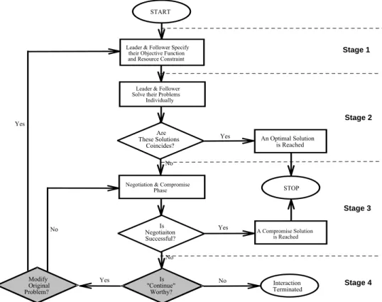
Figure 3, where the flow chart is shown, represents a common form of the interaction process. It is applicable for most collaborative cases and partial adversarial cases. In some cases that consist of the adversarial model (e.g. a relationship with extremely rare information sharing), the interaction process can differ from the one displayed in Figure 3 to such an extent that it cannot be formulated through bi-level programming techniques. This is the case when the interaction problem degenerates to a single-level multiple objectives problem due to the lack of partner’s information. Generally, Based on the flow chart shown in Figure 3, we divide the whole interaction process into four stages, where each stage can be described as follows:
START
Leader & Follower Specify their Objective Function and Resource Constraint
Leader & Follower Solve their Problems Individually Are These Solutions Coincides? Yes No
Negotiation & Compromise Phase An Optimal Solution is Reached STOP Is Negotiaiton Successful?
Yes A Compromise Solution is Reached No No Interaction Terminated Yes No Yes Stage 1 Stage 2 Stage 3 Stage 4 Is "Continue" Worthy? Modify Original Problem?
Figure 3: The flow chart of the supply-demand interaction Stage 1: Problem Formulation
At this stage, the preliminary structure of the supply-demand problem is formed, and key variables and interrelationship among these variables are identified. Both leader and follower indicate their requirements and limitations. These requirements and limitations can be directly transformed into corresponding objective functions and resource constraints within the problem. As a result, the supply-demand interaction can be formulated as the following BLMOP problem:
x
max
QL = [Q1L(x, y), Q2 L(x, y), …, Qk1 L(x, y)]T , (1a) xmin
SL = [S1L(x, y), S2L(x, y), …, Sk2L(x, y)]T, (1b) where ysolves:
y
max
QF = [Q1F(x, y), Q2 F(x, y), …, Qk3 F(x, y)]T, (1c)y
min
SF = [S1F(x, y), S2F(x, y), …, Sk4F(x, y)]T, (1d)subject to A1x+ A2y
≤
b, (2a)x, y
≥
0, (2b)where (QL; SL)T and (QF; SF)T are (k
1+k2)-dimensional and (k3+k4)-dimensional objective functions column
vectors, and are leader’s and follower’s objective function sets respectively. Q denotes quality and S denotes cost. The superscription L denotes leader and F denotes follower. Qi
L(x, y), i = 1, 2, …, k 1; Sj
L(x, y), j = 1, 2, …,
k2; QuF(x, y), u = 1, 2, …, k3; SvF(x, y), v = 1, 2, …, k4. x and y are n1-dimensional and n2-dimensional decision
variable column vectors and are respectively controlled by leader and follower. b is an m-dimensional constant column vector. Ar, r = 1,2 are m * nr constant matrices.
Stage 2: Individual Problem Solving
The leader and follower would each, on their own, carry out independent problem-solving procedures with regard to their problems. For example, the leader’s problem consists of objective functions (1a), (1b), and constraints (2a), (2b). The follower has its problem with objective functions (1c), (1d), and constraints (2a), (2b). It is important to note that both parties have multiple objective functions since there is always a trade-off between cost minimization and quality maximization. This means that, both the buyer and the supplier have to individually make compromises between their own conflicting objectives. According to Lee & Li [1993], the compromise solution to a multiple objective programming problem can be reached through applying the fuzzy
set theory [Zadeh, 1965; Zimmermann, 1996]. The decision maker first obtains the ideal and anti-ideal solution to their problem. For example, the ideal solution to leader’s problem can be obtained by solving each of his objective functions independently subject to the constraints in (2a) and (2b). Hence, leader’s ideal solution can be represented by
(I L)* = [(Q
1L)*, (Q2L)*,…, (Qk1L)*; (S1L)*, (S2L)*,…, (Sk2L)*]. (3)
The anti-ideal solution to leader’s problem can be obtained, subject to the constraints in (2a) and (2b), by minimizing the quality objective functions, QL, and by maximizing the cost objective functions, SL. Such an
anti-ideal solution can be represented by (I L)– = [(Q
1L)–, (Q2L)–,…, (Qk1L)–; (S1L)–, (S2L)–,…, (Sk2L)–]. (4) Then, the membership functions for leader’s objectives can be defined as:
)
(
LQ
i iµµµµ
= − −−
)
(
)
(
)
(
)
(
L L L L *Q
Q
Q
Q
i i i i-
y
x,
, i = 1, 2, …, k1, (5))
(
LS
j jµµµµ
= *)
(
)
(
)
(
)
(
L L L LS
S
S
S
j j j j−
−
− −y
x,
, j = 1, 2, …, k2. (6)Lee & Li used “min” operator, which was originally proposed by Zimmermann [1978], to aggregate the objective functions. It means that leader’s problem will be transformed into follows:
max λ (7) subject to
[
L(
)
−
(
L)
−]
/
[(
L)
*(
L)
−]
Q
Q
Q
Q
ix,
y
i i-
i≥
λ, i = 1, 2, …, k1,]
)
(
)
[(
/
)]
(
)
(
[
L L L L *S
S
S
S
j−
j j−
j − −y
x,
≥
λ, j = 1, 2, …, k2, A1x+ A2y≤
b, x, y≥
0, λ∈
{0,1}, where λ is defined as λ = j i,min
[µµµµ
i(
Q
iL)
,(
)
LS
j jµµµµ
]. (8)The leader can obtain its compromise solution by solving the problem in (7), and the follower can conduct similar procedure to obtain the compromise solution to his problem. After solving the problems at each side, the compromise solutions to leader and follower are [xL, yL, (QL)C, (SL)C] and [xF, yF, (QF)C, (SF)C], respectively.
Once the solutions to both sides coincide, that is, (xL, yL) = (xF, yF), the optimal solution is obtained, and the
interaction process is completed. If this is not the case, continue with Stage 3.
Stage 3: Negotiation and Compromise
Not only do the individual parties have to make a compromise between their own objectives about cost and quality, but the interaction between leader and follower is also a kind of bargaining which results in transactional decisions of the individual from a “give and take” process. The rarity of achieving an optimal solution makes this stage indispensable. At this stage, the leader may define the possible tolerance for the objectives and decision (the variables he controls) respectively through the application of fuzzy set theory (same as mentioned above) based on the ideal, anti-ideal and compromise solutions to his own problem obtained in Stage 2. The leader may also place weight on certain objectives according to his preferences and the degree of importance of the individual objective. By receiving information, such as the tolerance for the objectives and decision and the weights assigned to the individual objectives from leader, the follower can transform the information into the additional constraints of his own problem and then attempt to optimize his objectives. When such an optimization can be completed, the after results are to be forwarded to the leader. A compromise solution is achieved once the leader agrees with the result. This puts an end to the interaction process. If the opposite should be the case, then proceed with Stage 4.
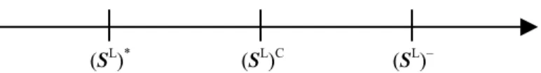
relationship. If the relationship model tends towards the collaborative then leader’s defined range of tolerance will be wider. In other words, leader will be more likely to consider follower’s situation and will adopt a strategy to ensure that both parties can simultaneously achieve acceptable level of satisfaction in the future. Conversely, if the relationship tends towards the adversarial model, leader’s defined range of tolerance will be narrower. It means that leader will be less likely to consider follower’s situation and will adopt a strategy to only ensure his achievement of high level of satisfaction. For example, considering leader’s objective of cost minimization, SL, it’s ideal, anti-ideal and compromise solutions are defined as [(SL)*, (SL)–, (SL)C]. If drawn as a line graph it will be represented in the following way:
Figure 4: The ideal, anti-ideal and compromise solutions to SL
The ideal and anti-ideal solutions to SL respectively stand for the lower and upper bounds of the possible value of SL. When the relationship model is of the collaborative type, then leader’s approach to SL‘s defined
range of acceptable value will lie in the area of [(SL)*, (SL)–]. It means that any value of SL smaller than (SL)–
will be acceptable for leader and the leader will reach the highest level of satisfaction when SL = (SL)*. On the
other hand, if this relationship model tends towards the adversarial type, then the leader as regards SL’s defined range of acceptable value will be situated in the area of [(SL)*, (SL)C]. It means that any value of SL smaller than
(SL)C will be acceptable for leader, and the leader will reach the highest level of satisfaction when SL = (SL)*.
The former means that leader provides follower with a good chance of achieving a higher level of satisfaction. This signifies that the interaction of both parties under these circumstances can lead to a smoother process. Conversely, if the latter situation prevails, leader will ask for higher standard for its future, causing follower’s satisfaction level to be lower. This will make it difficult for the interaction process to continue, and create a failure in the interaction. Furthermore, as the proceeding review of literature suggests, in a cooperative relationship both parties will pay greater attention to the success of the quality objective. On the other hand, in the case of an adversarial type, cost and price will be given priority consideration. The aforementioned phenomenon causes the objective function to have a different emphasis.
In other words, the leader can specify a minimum acceptable value (or maximum acceptable value) for specific objective function about quality, e.g. QL (or cost, e.g. SL). According to Shih et al. [1996], the
membership function for such an objective value will be trapezoid in shape depending on the nature of its minimization or maximization. Given the minimum acceptable value and maximum acceptable value for the objective function of QL and SL respectively, the membership functions for QL and SL can be formulated as
follows:
(i) When the type of relationship is collaborative:
)
(
LQ
i iµµµµ
=
≤
≤
<
−
≥
− − − −,
)
(
)
(
,
0
;
)
(
)
(
)
(
,
]
)
(
)
(
[
]
)
(
)
(
[
;
)
(
)
(
,
1
L L * L L L L * L L L * L LQ
Q
Q
Q
Q
Q
Q
Q
Q
Q
Q
i i i i i i i i i i iy
x
y
x
y
x
y
x
,
,
,
,
-
i = 1, 2, …, k1, (9))
(
LS
j jµµµµ
=
≥
≤
<
−
−
≤
− − − −,
)
(
)
(
,
0
;
)
(
)
(
)
(
,
]
)
(
)
(
[
)]
(
)
(
[
;
)
(
)
(
,
1
L L L L * L * L L L L * L LS
S
S
S
S
S
S
S
S
S
S
j j j j j j j j j j jy
x
y
x
y
x,
y
x
,
,
,
j = 1, 2, …, k2, (10)(ii) When the type of relationship is adversarial:
)
(
LQ
i iµµµµ
=
≤
≤
<
−
≥
,
)
(
)
(
,
0
;
)
(
)
(
)
(
,
]
)
(
)
(
[
]
)
(
)
(
[
;
)
(
)
(
,
1
C L L L L C L C L * L C L L L LQ
Q
Q
Q
Q
Q
Q
Q
Q
Q
Q
i i i i i i i i i i i * *y
x
y
x
y
x
y
x
,
,
,
,
-
i = 1, 2, …, k1, (11) (SL)* (SL)C (SL)–)
(
LS
j jµµµµ
=
≥
≤
<
−
−
≤
,
)
(
)
(
,
0
;
)
(
)
(
)
(
,
]
)
(
)
(
[
)]
(
)
(
[
;
)
(
)
(
,
1
C L L C L L L L C L L C L L L * *S
S
S
S
S
S
S
S
S
S
S
j j j j j j j j j j j *y
x
y
x
y
x,
y
x
,
,
,
j = 1, 2, …, k2, (12)On the other hand, however, the leader can specify tolerance pLfor decision x, and then the membership
function for x can be formulated as follows:
)
(x
xµµµµ
=
+
≤
<
−
+
≤
≤
−
−
−
,
0
;
,
/
]
)
[(
;
,
/
)]
(
[
L L L L L L L L L L L Lotherwise
,
p
x
x
x
p
x
p
x
x
x
p
x
p
p
x
x
(13)Such a membership function is called triangular fuzzy membership function since x is the triangular fuzzy number. It means that, for the leader, the acceptable interval of decision x is
x
L±
p
Lwith the highest level of satisfaction at x = xL. Moreover, the leader may also place particular weights on certain objectives according to his preferences and the relative importance of the individual objective. When using “min” operator for the intersection of fuzzy sets, the weighting of the membership functions for the objectives must be done inversely proportional to the weights proposed for each objective [Martinson, 1993]. Such a weighting method is also applicable for the follower in dealing with his problem.Hence, when both sides use the technique of weighting multiple objectives, the follower’s problem will be transformed into another problem embracing both sides’ membership functions of decisions and objectives, the weights assigned to the objectives, and the aggregated levels of satisfaction λ. In detail, assuming that the type of relationship is collaborative, the problem for the follower will become:
max λ (14) subject to A1x+ A2y
≤
b, (15a)p
p
x
x
(
L L)]
/
L[
−
−
≥
λI, (15b)p
x
p
x
L L)
]
/
L[(
+
−
≥
λI, (15c)p
p
y
y
(
F F)]
/
F[
−
−
≥
λI, (15d)p
y
p
y
F F)
]
/
F[(
+
−
≥
λI, (15e)]
)
(
)
(
[
/
]
)
(
)
(
[
Q
L−
Q
L − LQ
L *Q
L − i i i i ix
,
y
w
-
≥
λ, i = 1, 2, …, k1, (15f)]
)
(
)
(
[
/
)]
(
)
(
[
L L L L L *S
S
S
S
j−
j j j−
j − −w
y
x,
≥
λ, j = 1, 2, …, k2, (15g)]
)
(
)
(
[
/
]
)
(
)
(
[
F−
F − F F * F −Q
Q
Q
Q
ux
,
y
uw
u u-
u≥
λ, u = 1, 2, …, k3, (15h)]
)
(
)
(
[
/
)]
(
)
(
[
F F F F F *S
S
S
S
v−
v v v−
v − −x,
y
w
≥
λ, v = 1, 2, …, k 4, (15i) x, y≥
0, (15j) λ∈
[0,1], (15k)where (15d) and (15e) denote the membership functions of decision y controlled by the follower; (15h) and (15i) denote the membership functions of follower’s objectives; w denotes the weights assigned to objectives. The “min” operator is also used here to aggregate the preferred levels of satisfaction.
The follower can now try to optimize the above problem, and then submit the solution to the leader. If the leader accepts the solution, a compromised solution is reached, and the interaction process is finished. Or in other words, the conflict resolution is successful. If this is not the case, then go to the next stage. It is worth mentioning that the fuzzy set theory can be applied as expansively as possible. For example, the membership functions for specific constraints or the coefficient of specific variables can also be formulated depending upon the actual needs of the resolution process, although the objective and decision are the only applications illustrated in our problem. On the other hand, debate will arise when choosing “min” as an aggregate operator for simultaneously reaching the highest level of satisfaction since the “min” operator is non-compensatory and it does not guarantee a non-dominated solution [Lee & Li, 1993]. It is much more meaningful if a compensatory operator like the “arithmetical average”, “algebraic product”, or “algebraic sum” is applied in our problem to
obtain the compromise solution [Lee & Li, 1993; Shih et al., 1996].
Stage 4: Post-negotiation
Both leader and follower, especially the leader, have to consider at this stage whether to continue the interaction process or not. The so-called interaction failure results from the termination of the interaction, when either one of the parties lacks the incentive to go on. Otherwise, the parties involved have to decide whether to repeat the negotiations (e.g. to change relative tolerance, preferred level of satisfaction, or weights assigned to the individual objectives) or restart the entire process (e.g. to review the rationality and the accuracy of the original problem which leads to modification). This is worth to point out that this paper assumes that the antagonistic nature of the adversarial model frequently causes the results of the decision points at this stage (which is represented by the rhombic parts being shadowed in Figure 3) to lean towards the negative, or to even bypass such decision points to terminate the interaction process directly. This can occur as a result of the availability of multiple alternative transactional partners.
5. An Example
Supposing A Company commissions B Company to develop an EC system on its behalf. In regard to the system development, both parties must have related personnel participation. Thus speaking from the perspective of company A, there must be an input of compatible personnel to cooperate with B company’s system analysts and designers, so as to allow B Company to understand A Company’s system function requirements. B Company must input personnel with specialized knowledge and skill. In order to facilitate a smooth process, mutual personnel exchanges and on-site working must take place. For example, B Company’s system analysts and designers must go to A Company and engage in discussion and business process analysis, and provide customer query and consultation services, in order to resolve its key customer information system requirements. With regard to A Company, related personnel visits to B Company are required for education and training in the system management and technical maintenance. In regard to the cost of the employee engaging in on-site working, apart from it’s original subordinate enterprises having to pay for the related personnel costs, the company hosting the on-site working must also pay for the extra personnel costs.
In this example, we have established leader as A Company (the user of information service) it’s manpower participation is of two types (the variables it controls) divided into x1 and x2. And B Company is the follower
(the information service provider), it also provides two types of manpower participation: represented as y1 and y2.
The “man-hour” is a unit of manpower. Both leader and follower have two objective functions. Speaking from the minimum objective, both leader and follower wish that manpower costs be minimized. Each variable’s prior coefficient is its manpower cost per unit where a single unit is represented by “1000 dollars”. Especially worth mentioning is that, for every unit of y2 personnel that follower employs, it is eligible to receive governmental
financial assistance, and in this way it’s costs will be negative. From the perspective of the maximum objective, both follower and leader wish that the system has the highest level of quality. Leader’s considerations involve the greater use of its personnel (represented by x1 and x2) in order to sufficiently respond to the requirements of
its information system. Follower, from the perspective of achieving the highest level of quality, considers the greater use of its specialized technicians (y1) as necessary for achieving the greatest system effectiveness. In
regard to constraints, there are of two types: resource constraints and quality guarantee constraints. The resource constraint type is of five kinds: man-hour, working space, computing resource, administrative resources, and other supporting resources. Quality guarantee constraints are to be approved by both parties. In order to maintain a defined system development quality, every type of personnel combination must satisfy the time constraints. Combining all the above elements, this problem can be presented using the following bi-level multiple objectives programming problem:
max QL = x1 + x2 (16) min SL = 1.4 x1 + 0.9 x2 + 0.8 y1 + 0.3 y2 where y1, y2 solve: max QF = y1 min SF = 0.4 x1 + 0.2 x2 + 1.8 y1 – 0.2 y2 subject to x1
≤
530 x2≤
690 y1≤
430 y2≤
550(man-hour available per month)
2.2 x1 + 1.9 x2 + 1.8 y1 + 1.3 y2
≤
3400 (working space)0.8 x1 + 0.5 x2 + 2.5 y1 + 1.2 y2
≤
2350 (computing resource)2 x1 + 3.5 x2 + 1.4 y1 + 2.2 y2
≤
4000 (administrative resource)x1 + x2
≥
800y1 + y2
≥
650x1 + y1
≥
700x2 + y2
≥
950(quality guarantee constraints)
x1 , x2 , y1 , y2
≥
0whose constraint set is denoted by C. According to all the procedures outlined in section 4, the ideal and anti-ideal solutions to leader and follower’s problem can be obtained and they are: [(QL)*, (SL)*] = (1216.316, 1325),
[(QL)–, (SL)–]= (800, 1684.75), [(QF)*, (SF)*] = (430, 488), [(QF)–, (SF)–] = (170, 998.4). Following the above
result we can calculate that leader and follower’s individual compromise solutions respectively: [(QL)C, (SL)C;
x1L, x2L, y1L, y2L; λL] = (1037.9364, 1479.14276; 347.9364, 690, 352.0636, 297.9364; 0.5715) and [(QF)C, (SF)C;
x1F, x2F, y1F, y2F; λF] = (320.544, 702.8704; 379.456, 420.544, 320.5440, 550; 0.5790). According to individual
compromise solutions to both parties, it is realized that resolution to both sides does not correspond. Thus we have (x1L, x2L, y1L, y2L) ≠ (x1F, x2F, y1F, y2F). Because of this, supply and demand must proceed to the next step in
order to achieve a mutual compromise solution.
In the next step of the interaction, the leader can establish related membership functions for its objectives and then give them to follower to be used as the new constraints. On the other hand, the follower can establish related membership functions for its objectives. Assuming that the type of relationship is collaborative, the follower then needs to solve the following problem:
max λ (17) subject to c
∈
C, (18a) 1.4 x1 + 0.9 x2 + 0.8 y1 + 0.3 y2 + 359.75λ≤
1684.75, (18b) x1 + x2 – 416.316λ≥
800, (18c) 0.4 x1 + 0.2 x2 + 1.8 y1 – 0.2 y2 + 510.4λ≤
998.4, (18d) y1 – 260λ≥
170, (18e) λ∈
[0,1], (18f)where (18a) denotes the original constraint set. (18b) and (18c) are membership functions of leader’s objectives; (18d) and (18e) are membership functions of follower’s objectives. The compromise solution to above problem is (QL, SL, QF, SF) = (1015.294, 1498.7086, 304.4566, 734.4513) at (x
1, x2, y1, y2) = (395.5434, 619.7506,
304.4566, 478.6901) with the overall satisfaction of both parties λ= 0.5171. At this stage leader and follower can, in accordance with their individual preferences, establish their membership functions for individual objectives, and don’t need to follow their individual ideal, anti-ideal and compromise solutions. This study uses this method only for the purpose of convenient follow up comparison and explanation.
In addition, assuming that the leader’s control variable x1 is around 348 (based on its original, individual
compromise solution) with the negative and positive-side tolerance 20 and 50 respectively, then the following constraints will be added in (18):
x1 – 20λ
≥
328, (18g)x1 + 50λ
≥
398. (18h)Thus the compromise solution will become (QL, SL, QF, SF) = (1000.3484, 1511.6236, 326.062, 752.7746)
at (x1, x2, y1, y2) = (373.938, 626.4104, 326.062, 544.9715) with the overall satisfaction of both parties λ=
0.4812. On the other hand, the decision maker can, in accordance with its requirements, place particular emphasis on certain objectives according to his preferences and the relative importance of the individual objective. If leader differentiates in regard to its objectives, define the weight as: wQ=3, wS=1, the constraints (18b) and (18c) should be replaced by:
1.4 x1 + 0.9 x2 + 0.8 y1 + 0.3 y2 +359.75λ
≤
1684.75, (18i)x1 + x2 – 1248.948λ
≥
800, (18j)the new compromise solution will be (QL, SL, QF, SF) = (1076.9141, 1514.2227, 313.0859, 788.9374) at (x 1,
x2, y1, y2) = (386.9141, 690, 313.0859, 336.9141) with the overall satisfaction of both parties λ= 0.2217. For
the same reason, the follower can, in accordance to its own requirements, establish the membership functions for its control variable, place weights on its objectives, and then proceed to seek out the compromise solution. Accordingly, if such a compromise solution is acceptable to both leader and follower then the interaction process can be concluded. If one of the responsible parties is unable to accept it then they must proceed to the
next stage. It is worth to point out that, when the type of relationship is adversarial, there will be no feasible solution existed in our example. It means that no compromise solution can be achieved for both parties.
In the final stage, leader and follower must decide whether or not to continue with the interaction process. If the answer is no, then the process is terminated here. If they do decide to continue then they must decide whether to change the membership function or review the rationality and the accuracy of the original problem which leads to modification.
6. Discussions and Conclusions
According to different solutions to aforementioned problem, we can conclude that the more constraints (or membership functions) added into the problem, the lower overall level of satisfaction both parties will achieve. On the other hand, in the relationship with collaborative features, the defined range of tolerance of both parties will be wider. This contributes to future supply-demand interaction processes likelihood of achieving a higher level of satisfaction. Conversely, in an adversarial supply-demand relationship the defined range of tolerance of both parties will be narrower. This means that in future supply-demand interactions it will be difficult for both parties to achieve higher level of satisfaction or to reach a compromise solution.
This article was intended to outline some of the features of the association between the participating parties in the supply-demand interaction, and devise them into well-composed, solvable problems for easy follow-up analysis and comparison. We also methodically suggested an analytical method from an abstract to a concrete level. This method accurately portrays the supply-demand interaction by using bi-level programming technique and problem solving flow chart. A simplified example was used to illustrate the process of interaction (or problem solving). However, even though the method is young, it can be applied to explicit situations by changing certain assumptions to solve the specific problem properly. Although the optimal solution is rarely possible, a compromise solution, which is acceptable for all parties with conflicting objectives, provides conflict resolution. For other situations, the relationship may be ended where one party is disadvantaged and therefore reluctant to continue.
Both supplier and demander should base their decision on the company’s experience, criteria, past procedures in decision making, as well as an understanding of their internal practices and external environments such as the relationship with their potential associates in the interaction. This will help the company to reach a beneficial position in the interaction. On the other hand, this article wishes to emphasize the importance of information flow which carries the control mechanism. The reason why information sharing and exchange is crucial in affecting the interaction is because the interaction relies on the progressive exchange of information among decision units as the solution to the problem proceeds. Meanwhile, the difference between the many kinds of interactions is obviously discriminatory towards the amount of information shared and exchanged.
Acknowledgements
The authors would like to acknowledge the contribution of the three anonymous referees whose valuable comments and suggestions have contributed significantly to this paper.
REFERENCES
Adam, N. and Y. Yesha, “Strategic Directions in Electronic Commerce and Digital Libraries: Toward a Digital Agora,” ACM Computing Survey, Vol. 28, No. 4:818-835, 1996.
Alba, J., J. Lynch, B. Weitz, C. Janiszewski, R. Lutz, A. Sawyer, and S. Wood, “Interactive Home Shopping: Consumer, Retailer and Manufacture Incentives to Participate in Electronic Marketplaces,” Journal of Marketing, Vol. 61, No. 3:38-53, 1997.
Astley, G.W. and A.H. Van deVen, “Central Perspectives and Debates in Organization Theory,” Administrative Science Quarterly, Vol. 28, No. 2:245-273, 1983.
Bakos, J.Y., “A Strategic Analysis of Electronic Marketplaces,” MIS Quarterly, Vol. 15, No. 3:295-310, 1991a. Bakos, J.Y., “Information Links and Electronic Marketplaces: The Role of Interorganizational Information
Systems in Vertical Markets,” Journal of Management Information Systems, Vol. 8, No. 2:31-52, 1991b. Barbaro, L.M., “Medical Outcome Research: Another Frontier for Electronic Commerce,” EDI World, Vol. 6,
No. 4:26-30, 1996.
Bialas, W.F. and M.H. Karwan, “Two-level Linear Programming,” Management Science, Vol. 30, No. 8:1004-1020, 1984.
Bloch, M. and A. Segev, “The Impact of Electronic Commerce on the Travel Industry: An Analysis Methodology and Case Study,” Proceedings of the 30th Hawaii International Conference on System
Sciences (HICSS), Hawaii, 1997. [URL=http://www.stern.nyu.edu/~mbloch/docs/travel/travel.htm]
Brege, S., O. Branders, J. Lilliecreutz, and H. Branders, “Supplier Strategies in Buyer-Dominated Networks,” paper presented at The 9th IMP Conference, Bath, UK, September 1993.
Carter, J.R., L. Smeltzer, and R. Narasimhan, “The Role of Buyer and Supplier Relationships in Integrating TQM Through the Supply Chain,” European Journal of Purchasing & Supply Management, Vol. 4, No.
![Figure 1: Interactive buyer-supplier relationship with ISP’s mediation [Source: Tang et al., 1999]](https://thumb-ap.123doks.com/thumbv2/9libinfo/7546620.122164/3.892.233.665.659.917/figure-interactive-buyer-supplier-relationship-mediation-source-tang.webp)
![Figure 2: The classification of supply-demand interaction [Source: Tang et al., 2000]](https://thumb-ap.123doks.com/thumbv2/9libinfo/7546620.122164/4.892.247.645.470.743/figure-classification-supply-demand-interaction-source-tang-et.webp)