Augmented IFN learning model

JOURNAL OF COMPUTING IN CIVIL ENGINEERING / JANUARY 2000 / 15

A

UGMENTED

IFN L

EARNING

M

ODEL

By Shih-Lin Hung,

Member, ASCE, and J. C. Jan

ABSTRACT: Solving engineering problems is a creative, experiential process. An experienced engineer

gen-erally solves a new problem by recalling and reusing some similar instances examined before. According to such a method, the integrated fuzzy neural network (IFN) learning model was developed and implemented as a computational model for problem solving. This model has been applied to design problems involving a complicated steel structure. Computational results indicate that, because of its simplicity, the IFN model can learn the complicated problems within a reasonable computational time. The learning performance of IFN, however, relies heavily on the values of some working parameters, selected on a trial-and-error basis. In this work, we present an augmented IFN learning model by integrating a conventional IFN learning model with two novel approaches—a correlation analysis in statistics and a self-adjustment in mathematical optimization. This is done to facilitate the search for appropriate working parameters in the conventional IFN. The augmented IFN is compared with the conventional IFN using two steel structure design examples. This comparison reveals a superior learning performance for the augmented IFN learning model. Also, the problem of arbitrary trial-and-error selection of the working parameters is avoided in the augmented IFN learning model.

INTRODUCTION

Solving engineering problems — such as those of analysis and design — is a creative, experiential process in which the experiences and combined knowledge of engineers serve as resources. An experienced engineer generally solves a new problem in the following stages. First, he or she recalls in-stances that were similar but produced resolution, while prop-erly considering the functional requirements of those instances. Then, the engineer attempts to derive the solution from these similar instances through adaptation or synthesis. After the problem is solved, the new instance is then stored in her/his memory as an additional knowledge resource for solving fu-ture problems.

The described stages can be implemented as a computa-tional model for problem solving, one that utilizes a case base of previously solved problems when solving a new one. In symbolic artificial intelligence (AI), case-based reasoning (Carbonell 1981) is an effective means of facilitating computer program development. It attempts to solve problems by di-rectly accessing the case base. This approach relies on the explicit symbolic representation of a case base established from experience. With a given case base, case-based reasoning uses a representation involving specific episodes of problem solving, not only to solve a new problem, but also to learn how to solve the new problem. Based on the approach of case-based reasoning, the way to solve engineering problems has received considerable attention (Maher et al. 1995).

Artificial neural networks (ANNs), on the other hand, con-stitute a different AI approach, one that has made rapid ad-vances in recent years. Such networks have the ability to de-velop, from training instances, their own solutions to a class of problems. The method of representation used by ANNs, essentially a continuous function, is conducive to generaliza-tion beyond the original set of training instances used in their development. The feasibility of applying ANN computing to engineering problems has received increasing interest, partic-ularly on supervised neural networks with the

back-propaga-1

Assoc. Prof., Dept. of Civ. Engrg., National Chiao Tung Univ., 1001 Ta Hsueh Rd., Hsinchu, Taiwan 300, R.O.C.

2_{PhD Candidate, Dept. of Civ. Engrg., National Chiao Tung Univ.,}

1001 Ta Hsueh Rd., Hsinchu, Taiwan 300, R.O.C.

Note. Editor: Sivand Lakmazaheri. Discussion open until June 1, 2000. To extend the closing date one month, a written request must be filed with the ASCE Manager of Journals. The manuscript for this paper was submitted for review and possible publication on June 1, 1999. This paper is part of the Journal of Computing in Civil Engineering, Vol. 14, No. 1, January, 2000. qASCE, ISSN 0887-3801/00/0001-0015–0022/$8.00 1 $.50 per page. Paper No. 21139.

tion (BP, Rumelhart et al. 1986) learning algorithm. Vanluch-ene and Sun (1990) applied the back-propagation learning algorithm to structural engineering. Gunaratnam and Gero (1994) discussed the effect of the representation of input/out-put pairs on the learning performance of a BP neural network. Also, several other researchers have applied neural networks to engineering design and related problems (Hajela and Berke 1991; Ghaboussi et al. 1991; Kang and Yoon 1994; Stephen and Vanluchene 1994; Elkordy et al. 1994).

The learning processes of back-propagation (BP) supervised neural network learning models, however, always take a long time. Therefore, several different approaches have been de-veloped to enhance the learning performance of the BP learn-ing algorithm. Such an approach is to develop parallel learnlearn-ing algorithms on multiprocessor computers to reduce the overall computational time (Hung and Adeli 1991b, 1992, 1994b; Adeli and Hung 1993a). Another approach is to develop more effective neural network learning algorithms to reduce learning cycles (Adeli and Hung, 1993a, 1994a; Hung and Lin, 1994). A third approach involves the development of a hybrid learn-ing algorithm — for instance, by integratlearn-ing a genetic algo-rithm with neural network algoalgo-rithms to improve the overall learning performance (Hung and Adeli 1991b, 1994b).

Another category of learning in ANN includes unsupervised neural network learning models that are generally used in clas-sification problems (Carpenter and Grossberg 1988; Adeli and Hung 1993b). In structural engineering, Adeli and Park (1995) employed a counterpropagation neural network (CPN), which combines supervised and unsupervised neural networks, to solve complicated engineering design problems. That investi-gation concluded that a CPN learning model can learn how to solve complicated structural design problems within a reason-able computation time. Recently, authors Hung and Jan (1997, 1999) presented an integrated fuzzy neural network (IFN) learning model in structural engineering. The IFN learning model combined a novel unsupervised fuzzy neural network (UFN) reasoning model with a supervised neural network learning model using the adaptive L-BFGS learning algorithm (Hung and Lin 1994). The IFN learning model was applied to steel beam design problems. That work contended that the IFN learning model is a robust and effective ANN learning model. In addition, the IFN model can interpret a large number of instances for a complicated engineering problem within a rea-sonable computational time, owing to its simplicity in com-putation. However, the performance of the IFN learning model is heavily affected by some working parameters that are prob-lem dependent and obtained via trial and error.

In this work, we present a more effective neural network

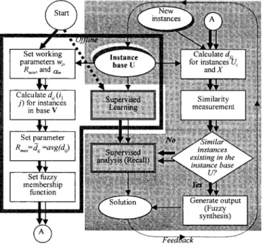
FIG. 1. Conventional IFN Learning Model

learning model, called the augmented IFN learning model, by integrating a conventional IFN learning model with two newly developed approaches. The first approach, correlation analysis in statistics, is employed to assist users in determining the appropriate working parameter to be used in the fuzzy mem-bership function. The second approach, self-adjustment in mathematical optimization, is used to obtain appropriate weights, systematically, for each decision variable required in the input of training instances. The novel model is imple-mented in C language on a DEC3000/600 workstation. The augmented IFN learning model proposed herein is applied to two structural engineering problems to verify its learning per-formance. The first example is a steel beam design problem. The second example involves the preliminary design of steel structure buildings. The two examples are also used to train a conventional IFN learning model, for the sake of comparison. REVIEW OF IFN LEARNING MODEL

This section briefly reviews the integrated fuzzy neural net-work (IFN) learning model (Hung and Jan 1997, 1999). The IFN learning model combines two sub-ANN learning models. One is a novel, unsupervised fuzzy neural network (UFN) rea-soning model: a single-layered laterally connected network with an unsupervised competing learning algorithm. The other is an offline assistant model: a supervised neural network learning model with the adaptive L-BFGS learning algorithm (Hung and Lin 1994). The IFN learning model is schemati-cally depicted in Fig. 1.

Assume that U is an associated instance base, with N solved

instances U1, U2, . . . , UN and X is a new instance. Instance

Ujis defined as a pair, including input Uj,iand its

correspond-ing output Uj,o. If there are M decision variables in the input

and K items of data in the output, the input Uj,iand output Uj,o

of instance Ujare represented as vectors of the decision

vari-ables and data, and are denoted as Uj,i= . . . , and

1 2 M

{u , u ,j j u }j

Uj,o= . . . , Similarly, the new instance X can also

1 2 K

{o , o ,j j o }.j

be defined as a pair including input Xi and unsolved output

Xo, respectively. The input Xiis a set of decision variables as

Xi= {x

1

, x2

, . . . , xM

}. The output Xois currently a null vector.

The learning stage in the IFN model is performed in two sub-ANN models concurrently. First, the offline assistant su-pervised neural network model is trained, based on the adap-tive L-BFGS supervised learning algorithm using these N given instances. In the UFN reasoning model, however, the learning process simply involves selecting appropriate work-ing parameters for the fuzzy membership function and weights for each decision variable in the input. The process is imple-mented in the following steps. The first step attempts to de-termine the degree of difference between any two distinct in-stances in base V, which contains P inin-stances randomly selected from instance base U. Therefore, a total of T = P=

C2

P(P2 1)/2 degrees of difference must be computed. The func-tion of degree of difference, diff (Ui,i, Uj,i), is employed to

mea-sure the difference, dij, of two inputs Ui,iand Uj,ifor instances

Uiand Ujin V. The function is defined as the modified square

of Euclidean distance and represented as

M

m m 2

d = diff (U , U ) =ij i,i j,i

O

m =1

where wi and am denote predefined weights and are used to

represent the degree of importance for the ith instance in the instance base for the mth decision variable in the input. The weights wiare generally set as constant one. The weightsam,

however, are set by trial and error. After the values of dijfor

all instances in base V are computed, the average of the sum of dij, denoted as = avg(dij) = (dij)/T, can be computed.

T

¯dij (t =1

The second step entails determining the fuzzy membership function. The relationship of ‘‘similarity’’ between any two instances is represented using a fuzzy membership function. In the UFN reasoning model, a quasi-Z-type membership func-tion is used and defined as

m(d ) = f(R , R , d )ij max min ij

0 if dij$ Rmax

RmaxRmin2 R dmin ij

=

H

(Rmax2 R )dmin ij

1 if dij# Rmin (2)

The terms Rmaxand Rminare two working parameters that define

the upper and lower bounds of ‘‘degree of difference.’’ The lower bound Rminis set as a constant 10

25_{. The upper bound,}

however, is set as Rmax = hd .¯ij The term h is a real number

between zero and one and it was set by trial and error. Con-sequently, the degree of similarity for instances Uiand Ujcan

be determined from the fuzzy membership function.

After learning in the UFN and in the assistant supervised learning model is completed, any new instance X can be solved via the IFN learning method. The reasoning in UFN is per-formed through a single-layered, laterally connected network with an unsupervised competing algorithm, and it is imple-mented in three steps. The first step involves searching for some instances from the instance base U that resemble the new instance X according to their inputs; that is, the degree of dif-ference, dXj, between the inputs, Xiand Uj,i, for instance X and

instance Uj in base U is calculated. The input Xi of instant X

is presented to the first node and the input Uj,i of instance Uj

JOURNAL OF COMPUTING IN CIVIL ENGINEERING / JANUARY 2000 / 17

FIG. 2. Example of Accumulative Correlation Curve

is presented to the ( j1 1)th node simultaneously. The degree of difference dXjis then computed using (1) as diff (Xi, Uj,i) =

am(wxx m ₂

The second step entails representing

M m 2

(m =1 w u ) .j j

the relationships among the new instance and its similar in-stances, with dXjless than Rmax. The fuzzy set,Ssup,X,of ‘‘similar

to X ’’ was then expressed as follows:

Ssup,X= (m /S ) 1 (m /S ) 1 ??? 1 (m /S ) 1 ???1 1 2 2 p p (3)

where Sp = pth similar instance to instance X; the term ‘‘1’’

denotes a union operator; andmp= corresponding fuzzy

mem-bership value.

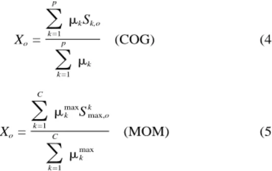
The final step involves generating the output Xo vector of

instance X by synthesizing the outputs of its similar instances according to their associated fuzzy membership values using center of gravity (COG) or mean of maximum (MOM) meth-ods (Hung and Jan 1999). For the given unsolved instance X, assume that P similar instances are in fuzzy set Ssup, x; they are

classified into C distinct clusters according to their outputs. Then, the output Xoof instance X yielded via these two

meth-ods are defined, respectively, as follows:

p m Sk k,o

O

O

O

O

where mk denotes the membership value for the kth similar

instance in fuzzy set Ssup, x. Correspondingly, denotes the max

mk

membership value for the most similar instance k in the kth Smax

cluster.

The reasoning process of the UFN depends on determining the degree of similarity among X and Uj. Consequently, no

solution can be generated by the UFN reasoning model if the new instance entirely differs from all instances in the instance base, e.g., all dXi are greater than Rmax. In addition, using

in-appropriate working parameters would allow for the possibility that no similar instances can be derived. For the above issues, the undertrained adaptive L-BFGS supervised neural network is used as an assistant system to generate an approximate out-put for the new instance.

AUGMENTED IFN LEARNING MODEL

In the conventional IFN learning model, working param-eters (such as wj,am, Rmax, and Rmin) are selected subjectively

by users, and generally, on a trial-and-error basis. Conse-quently, the learning performance is highly affected by these parameters, especially Rmax and am. In this work, two novel

approaches are employed for assisting the users to determine these parameters and weights systematically. One approach, correlation analysis in statistics, is used to determine the ade-quate Rmax value in the fuzzy membership function. The other

approach, self-adjustment based on mathematical optimization theory, is employed to find proper values for weightsam.

Correlation Analysis for Rmaxin Fuzzy

Membership Function

In conventional IFU, the similarity measurement between two instances heavily depends on the value of parameter Rmax.

A small value of Rmaximplies that a strict similar relationship

between instances is utilized. Consequently, most of the stances are sorted as dissimilar. As a result, few similar

in-stances to the new instance can be found and, ordinarily, no solution can be generated via the UFN reasoning model. On the other hand, a loose similar relationship is adopted under the case of a larger Rmax. Accordingly, a large number of

in-stances are taken to be ‘‘similiar inin-stances’’ and the solution generated via these similar instances is inferior. Here, the lin-ear correlation analysis in statistics is employed to facilitate the determination of appropriate value of Rmax in the fuzzy

membership function. The analysis is a process that aims to measure the strength of the association between two sets of variables that are assumed to be linearly related.

For the above instance base U with N instances, the corre-lation analysis in the fuzzy membership function is imple-mented in the following steps. The first step is to determine the degree of difference between any two instances in the base

U using the aforementioned function of degree difference in

(1). Hence, a total of 1 N) resembling samples Sij(Ui,o, N

(C2

Uj,o, dij) can be compiled. A resembling sample contains two

instances’ outputs (Ui,oand Uj,o) and the corresponding degree

of difference (dij). Thereafter, two arrays, At and Bt, can be

assorted from resembling samples in the case of dijless than

or equal to a prescribed value, say t. The elements in At and

Bt are the first and second items, respectively, of these

resem-bling samples. Next, the accumulative correlation coefficient, AcoCORREL(At, Bt, t), is calculated for arrays At and Btwith

the degree of difference less than or equal to t. Assume that for a total P resembling samples with dijless than a prescribed

t, the arrays At and Bt can be denoted as

A = {at kua = U [ S , for d # t} = {a , a , . . . , a }k i,o ij ij 1 2 p

B = {bt kub = U [ S , for d # t} = {b , b , . . . , b }k j,o ij ij 1 2 p

The value of the accumulative correlation coefficient equals

Cov(A , B , t)t t AcoCORREL(A , B , t) =t t (6) s sAt Bt p 1 Cov(A , B , t) =t t

O

wheresA_tand sB_t are standard errors of arrays At and Bt;mA_t

andmB_tare the means of At and Bt. The formulas expressed in

(6) and (7) represent the relationship between the accumulative correlation coefficient to any value of t. An accumulative cor-relation curve can be plotted as a function of t and Ac oCOR-REL(At, Bt, t). Fig. 2 demonstrates an accumulative correlation

curve for two arrays At = sin (x) and Bt = 0.95(x 2 x

3

/3!1 x5

/5!) such that x =2p 1 (p/15)i, i = 0 to 30. Shown in Fig. 2, the curve falls from one to zero as the value of t increases, and it resembles the quasi-Z-type fuzzy membership function defined in (2) for the case of Rminequal to zero. Note that the

FIG. 3. Augmented IFN Learning Model

appropriate Rmaxequals a certain value of t, such that instances

in the instance base U have a certain degree of correlation. Obviously, the smaller the t implies a larger accumulative correlation coefficient, indicating a strong relationship between the two arrays, e.g., the strongest correlation, t = 0, between the two arrays refers to the case in which the instances in the two sets are identical and the value of AcoCORREL(At, Bt, t)

equals one. In such a case, no solution to a new instance can be generated via the UFN reasoning model except for when identical instances exist in the instance base. In order to avoid this issue here, we set AcoCORREL(At, Bt, t) equal to 0.8 as

the lower bound for similarity measurement. The value of t corresponding to this lower bound is adopted as the appropri-ate value of Rmax.

Self-Adjustment Approach for Selecting Weightsam

Except for Rmax, the selected weightsam also significantly

affect the learning performance for the conventional IFN. This occurrence has been investigated in the earlier work (Hung and Jan 1999). The learning results indicated that significant improvements were achieved as the weights were gradually updated via a basis of heuristic knowledge associated with learning problems. In this study, a more systematical approach — self-adjustment based on mathematical optimization — is adopted to facilitate the search for appropriate weights.

For the above instance base U with N instances, the self-adjustment approach can be briefly stated as consisting of the following steps. First, set up the corresponding working pa-rameters, Rmax, Rmin, and wj, where Rmax is determined using

the aforementioned correlation analysis approach and where parameter Rminand weights wjare set as constants in this work.

Meanwhile, weightsamfor each decision variable in the input

are directly initialized as one. Then, based on these working parameters, the outputs for training instances are found via the UFN reasoning model. Then the error, Ei, between the

com-puted and desired outputs, Y and Ui,o, for training instance Ui,

is calculated. The system error, E, for a total N instances is then defined as half of the average sum of errors and denoted as N 1 E =

O

O

= kth items of data in desired and computed

k

oi

outputs, Ui and Y, respectively. Note that the system error is

an implicit function of the weightsam as E(am).

Weights am in the UFN reasoning model are adjusted to

reduce the system error as much as possible. This goal can be achieved if a set of appropriate weights, am, are used. The

problem, then, can be considered as an unconstrained opti-mization problem, that is, searching a set of optimum weights by iteration to minimize the system error. In the mathematical optimization approaches, the conjugate gradient (CG) method has been proved an efficient means of solving the problem. The weights am are updated in each iteration, say the (s 1

1)th iteration, as_a(s11)=_a(s)1_{ld .}(s) The terml is step length

m m

and is set as a constant in this work. The search direction is defined as (s) d (s) (s) (s) d = g =2=E(a ) if s = 0m (10a,b)

H

The iteration is terminated as the value of ig(s11)i or

2 is sufficiently small. The term is the

(s11) (s) (s)

uE(am ) E(a )um g

negative gradient vector of function E(am). For simplicity, the

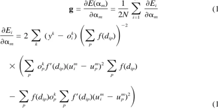
superscript (s), denoted as the sth iteration, is ignored. Here-inafter, vector g is derived using chain rule and denoted as

N ­E(a )m 1 ­Ei g = =

O

O

SO D

SO

O

O O

D

where index p denotes the pth similar instance in fuzzy set and indices m and k denote the mth decision variable Ssup, U_i,

in the input and the kth data item in the output vectors, re-spectively.

Augmented IFN Learning Model

In this section, we present an augmented IFN learning model. Fig. 3 schematically depicts the procedures of the aug-mented IFN learning model. Instead of using a constant work-ing parameter Rmax, as in conventional IFN, the appropriate

parameter is determined using correlation analysis. Mean-while, the appropriate weightsamare adapted during the

self-adjustment process through a mathematical approach. These two approaches, called self-organized learning, are used to en-hance the learning capability of the conventional IFN learning model. The procedure of the augmented IFN learning model can be summarized as follows:

• Self-organized learning phase

Step 0. Train the adaptive supervised L-BFGS learning neural network model offline.

Step 1. Initialize parameter Rmin as constant 1025 and

JOURNAL OF COMPUTING IN CIVIL ENGINEERING / JANUARY 2000 / 19 weight am for each decision variable, on a heuristic

basis or by trial and error.

Step 2. Calculate the degree of difference dij(i ≠ j)

among all instances in base V.

Step 3. Determine the parameter Rmaxusing correlation

analysis and set Rmax = t such that AcoCORREL(At, Bt,

t) = 0.8.

Step 4. Set the fuzzy membership function, m(dij) =

f (Rmin, Rmax, dij), defined in (2).

Step 5. Adjust the weightamfor each decision variable

in input, using the self-adjustment approach. • Analysis phase (after learning phase is completed)

Step 6. Present the new (unsolved) instance X to the UFN reasoning model, and perform a similarity mea-surement between X and instance Uiin the base U using

a single-layered, lateral-connected competing network. Step 7. If more than one similar instance is found in Step 6, generate the solution Xo for the new instance

using fuzzy synthesis approaches in (4) or (5), and go to Step 9. Otherwise go to next step.

Step 8. Compute the solutions via the undertrained as-sistant adaptive L-BFGS supervised learning model and go to next step.

Step 9. Feedback the new instance into the base U. Meanwhile, further learning in the assistant supervised learning model is launched offline.

APPLICATIONS

Here the novel augmented IFN learning model is applied to problems of engineering design. Two structural design exam-ples are presented to verify the learning performance of the augmented IFN learning model. The first example is a steel beam design problem. The second is the preliminary design of steel structure buildings. The two examples are also used to train a conventional IFN learning model for comparison.

Steel Beam Design Problem

The problem is the design of the lightest W-section simply supported steel beam with compact section, under LRFD Spec-ification (Manual 1994). The problem was studied in our ear-lier work (Hung and Jan 1999), with those results demonstrat-ing that the conventional IFN learndemonstrat-ing model is superior to a stand-alone supervised neural network with L-BFGS learning algorithm when the number of training instances was large enough. This work investigates only the learning performances of the conventional IFN and the novel augmented IFN learning models.

The LRFD design method, applied to the effect of lateral torsional buckling for beam with compact section, is summa-rized in the following steps:

1. Determine the factored moment Muat midspan of a given

beam.

2. Select one potential member with plastic section modu-lus Z so that the required nominal moment Mn= Zfy

sat-isfies 0.9Mn$ Mu, where fyis the specified yield strength

of the beam.

3. Estimate whether the lateral supports are close enough to design the beam using plastic analysis or whether we should use the fully plastic moment strength Mpwithout

plastic analysis, for a given unbraced length Lb. The

nominal moment Mn is then obtained according to the

following formulas with different conditions:

a. If L < L ,b p then M = Mn p b. If L < L < L ,p b r then Mn = C [Mb p2 (M 2 M )((L 2 L /L 2 L ))] # Mp r b r r p p c. If L > L , then Mb r n 2 p pE = M = Ccr b

Î

S D

where Mp= plastic moment strength; Lpand Lr= limited

laterally unbraced length for full plastic bending capacity and for inelastic lateral-torsional buckling, respectively; Cb= moment gradient coefficient; Mr= limited buckling

moment; E = elasticity modulus of steel; Cw= warping

constant; Iy = moment of inertia about the minor axis;

G = shear modulus of elasticity of steel; and J = torsional constant.

4. Finally, confirm whether or not the section of selected member satisfies the requirements of flexural design strength, 0.9Mn $ Mu, and shear design strength, 0.9Vn

$ Vu, where Vnis the nominal shear strength.

The above steps are repeated until a satisfactory lightest mem-ber is obtained. Eight hundred instances, created according to the aforementioned design process, are used in the present ex-ample to train and verify the conventional and augmented IFN learning models. Of these, 600 are used as training instances and the remaining two hundred (200) are used as verification instances. Seven decision variables are used as inputs in order to determine the plastic modulus Z of a lightest W-section steel beam with compact section. The seven decision variables are the yielding strength of steel fy, factored maximum bending

moment Mu, the live load wl, the factored maximum shear

force Vu, the span of the beam L, the moment gradient

coef-ficient Cb, and the unbraced length Lb. Notably, the first

de-cision variable, fy, was not used in the earlier work (Hung and

Jan 1999), as the yielding strength of steel was identical for each instance.

The parameters Rminand wiare set as constant 1025and one,

respectively. The weightsam, however, are initialized as [1, 9,

1, 1, 1, 1, 1] for the seven decision variables. Of these, the second weight, a2, for decision variable, factored maximum

bending moment Mu, is set based on the finding investigated

in the earlier work (Hung and Jan 1999). Using these param-eters and weights, the augmented IFN learning model is trained in four different cases with different numbers of train-ing instances in base V. The number of traintrain-ing instances is increased from 100 to 400 with an increment of 100. After performing the correlation analysis in four different bases of

V, the accumulative correlation coefficients can be computed

with respect to any specified value t. With the value of Aco CORREL(At, Bt, t) equal to 0.8, the values of t(=Rmax) for four

different cases are obtained. Those values are 0.044, 0.034, 0.033, and 0.030, respectively, for 100, 200, 300, and 400 training instances in base V, and are displayed in Fig. 4. In-terestingly, according to this figure, the greater the number of instances in bases V implies a higher correlation among these instances. Restated, the value of Rmax decreases with an

in-crease of the number of training instances. After the value of Rmax is determined, the self-adjustment approach is launched

to search the appropriate weightsamfor each decision variable

in the input.

After self-adjustment is achieved, a set of weights am is

obtained, e.g., the weights am are adjusted to values [1.42,

6.93, 1.02, 1.01, 1.01, 1.51, 0.73] for the case of V with 400 training instances. Note that the first, second, and sixth weights (a1,a2, anda6) are changed by more than the other weights.

These adjustments illustrate that the first and sixth decision

FIG. 4. Accumulative Correlation Curve for Steel Beam De-sign Example

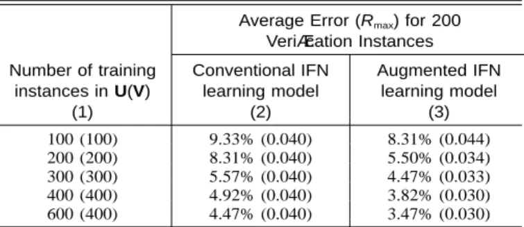
TABLE 1. Results of Steel Beam Design Problem

Number of training instances in U(V)

(1)

Average Error (Rmax) for 200 Verification Instances Conventional IFN learning model (2) Augmented IFN learning model (3) 100 (100) 9.33% (0.040) 8.31% (0.044) 200 (200) 8.31% (0.040) 5.50% (0.034) 300 (300) 5.57% (0.040) 4.47% (0.033) 400 (400) 4.92% (0.040) 3.82% (0.030) 600 (400) 4.47% (0.040) 3.47% (0.030)

FIG. 5. Comparison of Computed and Desired Outputs for Verification Instances: Steel Beam Design Example

variables, fyand Cb, are more important than we would be led

to believe by a process of trial and error. However, the weight

a2 for the second decision variable, Mu, is adjusted from 9 to

6.93. The occurrence reveals that the factored moment, Mu, is

the most important decision variable in the input, as compared with other decision variables. Then, the 200 verification in-stances are used to verify the learning performance of the con-ventional and augmented IFN learning models. The verifica-tion in the augmented IFN is based on the newly adjusted weightsamwith the appropriate Rmax. The working parameters

and weights used in the conventional IFN, however, are se-lected by trial and error. Fig. 5 compares the computed and desired outputs of the 200 verification instances for the aug-mented and conventional IFN learning models. The correlation coefficients for the computed and desired outputs are 0.997 and 0.992 for the augmented and conventional IFN learning model, respectively. Table 1 summarizes the computing results

for the 200 verification instances. According to this table, the learning performance is improved as the number of training instances increases for the augmented and conventional IFN learning models. This same table reveals that the average er-rors for verification instances are 3.47% and 4.47% for the augmented and conventional IFN learning models, respec-tively. In sum, the learning performance of the augmented IFN learning model is much better than that of the conventional IFN learning model in this example.

Based on the newly adjusted weights am, correlation

anal-ysis is next performed for the case of 400 instance bases in V again. According to those results, the accumulative correlation coefficients are higher for any specified value t than those ob-tained from the initial set of weights. For example, the accu-mulative correlation coefficient is from 0.8 to 0.9 at the value t equal to 0.03 (Fig. 4).

Preliminary Design of Steel Structural Buildings In the complete design of a structure, the preliminary design stage is mainly a creative, experiential process that involves the choice of structure type, selection of the material, and de-termination of the sections of beams and columns in the struc-ture. An experienced engineer is likely to carry out this stage more quickly than does an inexperienced one. The basic con-figuration of the structure at this stage should satisfy the spec-ified design code, such as LRFD for steel structures. To satisfy the prescribed constrains and achieve minimum expenditure for materials and construction, this stage becomes a looped optimization decision-making process. Hence, a good initial development of the basic form, with sections of beams and columns satisfying the aforementioned constraints, will reduce the number of redesign cycles. After a basic structure is de-termined, the structural analysis stage involves analyzing the initial guessed structure and computing the service loads on the members. Also, the maximum lateral drift of the structure and the drifts between floors are computed if lateral loads are considered. The present example involves a complete design structure that satisfies the conditions that the service loads should not exceed the strength of the members; the drifts should be within the prescribed limits, and the structure should be economical in material (e.g., minimum weight), construc-tion, and overall cost. In this example, the augmented IFN learning model is trained to learn how to implement the pre-liminary design of buildings satisfying the conditions of utility, safety, and economy in only one design cycle. For simplicity, only regular buildings with a rectangular layout — such as most factory buildings — are considered herein. Also, the beams in every floor have the same sectional dimensions, as do the columns.

In this example, 416 instances are used. They are randomly divided into 380 training instances and 36 verification in-stances. Seven decision variables are used as inputs to deter-mine the sections of beams and columns of a building that satisfies the given specifications. The seven decision variables and their limits are described as follows:

1. Number of stories = [9, 10, 11, 12, 13, 14, 15]

2. Bay length in long-span direction (X direction) = 9 to 12 m

3. Bay length in short-span direction (Y direction) = 6 to 9 m

4. Number of bays in both directions = [3, 4, 5] 5. Seismic zone coefficient = [0.18, 0.23, 0.28, 0.33] 6. Live load (kgw/m2

) = 200 to 350 7. Wall load (kgw/m) = [100, 200]

Other corresponding decision variables used in the stage of preliminary design are assumed to be constant. In practice, the

JOURNAL OF COMPUTING IN CIVIL ENGINEERING / JANUARY 2000 / 21

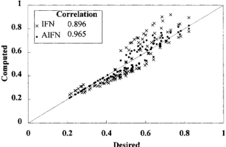
FIG. 7. Comparison of Computed and Desired Outputs (Beams) for Verification Instances: Preliminary Design of Steel Structural Buildings

FIG. 8. Comparison of Computed and Desired Outputs (Col-umns) for Verification Instances: Preliminary Design of Steel Structural Buildings

TABLE 2. Results of Preliminary Structural Design Problem

Error (%)

(1)

NUMBER OF ITEMS IN OUTPUT FOR VERIFICATION INSTANCES Conventional IFN Learning Model Beam (2) Column (3) Augmented IFN Learning Model Beam (4) Column (5) 0; 5 12 43 52 51 5; 10 29 29 39 31 10; 15 21 22 13 20 15; 20 29 10 3 6 >20 17 4 1 0

Average error for 36

ver-ification instances 13.81% 9.36% 6.10% 6.17%

Note: Each instance has six items, three beams, and columns, in out-put.

FIG. 6. Accumulative Correlation Curves for Example of Pre-liminary Design of Steel Structural Buildings

sections of beams and columns of a building are classified into certain groups for convenience in construction, instead of sep-arate consideration being given to each element. Here, a build-ing with three groups of steel elements in both beams and columns is considered. The three groups are upper, medium, and lower. For a building with N stories, these three groups are defined as upper group: floors from 2N/3 to N; medium group: floors from N/3 to 2N/3; and lower group: floors from one to N/3. An instance contains seven decision variable inputs and six data items as outputs.

The parameters Rminand wiare set as constant 10

25_{and one,}

respectively. The weightsam, however, are initialized as [1, 1,

1, 1, 1, 1, 1] for the seven decision variables. Using these parameters and weights, correlation analysis in the augmented IFN learning model is performed first to determine the work-ing parameter Rmax. Fig. 6 displays the result of correlation

analysis. With the value of AcoCORREL(At, Bt, t) equal to 0.8,

the values of t(=Rmax) are obtained. They are 0.12 for beams

and 0.178 for columns, respectively.

After the fuzzy membership function is defined, the self-adjustment approach is launched to obtain the adequate weightsamfor each decision variable in the input. The weights

am for each decision variable are updated from [1, 1, 1, 1, 1,

1, 1] to [1.471, 1.369, 0.416, 0.008, 1.104, 0.825, 0.513] for beams and to [1.106, 0.997, 0.542, 0.009, 1.232, 0.999, 0.997] for columns. Interestingly, the weights of the fourth decision variable in beams and columns are both self-adjusted close to zero. This observation indicates that this decision variable (number of bays in both directions) is insignificant in the input. Consequently, this decision variable can be neglected. The 36 verification instances are used to verify the learning perfor-mance of the augmented and conventional IFN learning mod-els, respectively. Notably, the augmented IFN is verified on the basis of the newly adjusted weightsam with the adequate

Rmax. The working parameters and weights used in the

con-ventional IFN, however, are selected on a trial-and-error basis. Fig. 7 depicts the correlation between the computed and de-sired outputs of beams for the 36 verification instances for the augmented as well as conventional IFN learning models. Sim-ilarly, Fig. 8 displays the correlation between the computed and desired outputs for columns for the thirty-six verification instances using the two IFN learning models. Table 2 sum-marizes the learning results for thirty-six verification instances. According to this table, the average percentage errors for beams and columns are 13.81 and 9.36 for the conventional IFN learning model. However, these errors are reduced to 6.17 and 6.1 for beams and columns, respectively, for the aug-mented IFN learning model. The augaug-mented IFN learning model significantly improves in terms of learning. This

ex-ample also illustrates that the augmented IFN learning model yields a substantially better learning performance than that of the conventional IFN learning model.

CONCLUDING REMARKS

This work presents an augmented IFN learning model by integrating two newly developed approaches into a conven-tional IFN learning model. These approached are a correlation analysis in statistics and self-adjustment in mathematical

timization, which collaboratively enhance the learning capa-bility of the conventional IFN. The first approach, correlation analysis in statistics, assists users in determining the appro-priate working parameter used in the fuzzy membership func-tion. The second approach, self-adjustment in mathematical optimization, obtains appropriate weights, systematically, for each decision variable in the input of training instance. The augmented IFN learning model proposed herein is applied to engineering design problems. Two structural design problems were addressed to assess the learning performance of the aug-mented IFN learning model. Based on the results of this work, we can conclude the following:

1. The problem of arbitrary trial-and-error selection of the working parameter (Rmax) in fuzzy membership function,

encountered in the conventional IFN learning model, is avoided in the newly developed augmented IFN learning model. Instead of arbitrary Rmax, the appropriate value of

Rmaxis determined using correlation analysis in statistics.

Thus, the new learning model provides a more solid sys-temic foundation for IFN learning than the conventional IFN learning model.

2. In the conventional IFN learning model, the weightsam,

denoting the importance of the mth decision variable in the input, are set on a trial-and-error basis. For compli-cated problems, the appropriate weights are difficult to obtain because of a lack of the relevant heuristic knowl-edge. In due course, the value is commonly initialized as one for most of the examples. This problem is avoided by the newly developed learning model. Instead of an assumed constant, the appropriate weights are deter-mined through the self-adjustment approach in mathe-matical optimization. Therefore, the augmented IFN learning model provides a more solid mathematical foun-dation for neural network learning.

3. For each training instance, decision variables in the input are generally selected subjectively by users. As a result, some trivial decision variables may be adopted in the input for some complicated examples. Based on the self-adjustment approach, the importance of a decision vari-able in an input can be derived systematically. Therefore, insignificant or redundant decision variables in the input can be neglected.

4. The results illustrate that the value of the appropriate Rmax

gradually falls with an increase in the number of in-stances. Consequently, not only is the learning perfor-mance for training instances enhanced, but also the per-formance for verification instances is improved. Notably, a small value of Rmax indicates that a strict similarity

measurement is utilized in the UFN reasoning model and the possibility that no similar instances can be derived for any new instance also increases.

ACKNOWLEDGMENTS

The writers would like to thank the National Science Council of the Republic of China for financially supporting this research under Contract No. NSC 86-2221-E-009-070.

APPENDIX. REFERENCES

Adeli, H., and Hung, S. L. (1993a). ‘‘A concurrent adaptive conjugate gradient learning on MIMD machines.’’ J. Supercomputer Appl., 7(2), 155–166.

Adeli, H., and Hung, S. L. (1993b). ‘‘A fuzzy neural network learning

model for image recognition.’’ Integrated Computer-Aided Engrg., 1(1), 43–55.

Adeli, H., and Hung, S. L. (1995). Machine learning—neural networks, genetic algorithms, and fuzzy systems. Wiley, New York.

Adeli, H., and Park, H. S. (1995). ‘‘Counterpropagation neural network in structural engineering.’’ J. Struct. Engrg., ASCE, 121(8), 1205– 1212.

Carbonell, J. G. (1981). ‘‘A computational model of analogical problem solving.’’ Proc., 7th Int. Joint Conf. on Artificial Intelligence, William Kaufmann, Los Altos, Calif., 1, 147–152.

Carpenter, G. A., and Grossberg, S. (1988). ‘‘The ART of adaptive pattern recognition by a self-organizing neural network.’’ IEEE Comp., 21, 77–88.

Elkordy, M. F., Cheng, K. C., and Lee, G. C. (1994). ‘‘A structural dam-age neural network monitoring system.’’ Microcomp. in Civ. Engrg., 9(2), 83–96.

Ghaboussi, J., Garrett, J. H., and Wu, X. (1991). ‘‘Knowledge-based mod-eling of material behavior and neural networks.’’ J. Engrg. Mech., ASCE, 117(1), 132–153.

Gunaratnam, D. J., and Gero, J. S. (1994). ‘‘Effect of representation on the performance of neural networks in structural engineering applica-tions.’’ Microcomp. in Civ. Engrg., 9(2), 97–108.

Hajela, P., and Berke, L. (1991). ‘‘Neurobiological computational modes in structural analysis and design.’’ Comp. and Struct., 41(4), 657–667. Hung, S. L., and Adeli, H. (1991a). ‘‘A model of perceptron learning with a hidden layer for engineering design.’’ Neurocomputing, 3(1), 3–14. Hung, S. L., and Adeli, H. (1991b). ‘‘A hybrid learning algorithm for

distributed memory multicomputers.’’ Heuristics—J. of Knowledge Engrg., 4(4), 58–68.

Hung, S. L., and Adeli, H. (1992). ‘‘Parallel backpropagation learning algorithms on Cray Y-MP8/864 supercomputer.’’ Neurocomputing, 5(6), 287–307.

Hung, S. L., and Adeli, H. (1994a). ‘‘An adaptive conjugate gradient learning algorithm for effective training of multilayer neural net-works.’’ Appl. Math. and Computat., 62(1).

Hung, S. L., and Adeli, H. (1994b). ‘‘A parallel genetic/neural network learning algorithm for MIMD shared memory machines.’’ IEEE Trans. on Neural Networks, 5(6), 900–909.

Hung, S. L., and Lin, Y. L. (1994). ‘‘Application of an L-BFGS neural network learning algorithm in engineering analysis and design.’’ Proc., 2nd Nat. Conf. on Struct. Engrg., Vol. III, Chinese Society of Structural Engineering, Taipei, Taiwan, 221–230 (in Chinese).

Hung, S. L., and Jan, J. C. (1997). ‘‘Machine learning in engineering design—an unsupervised fuzzy neural network learning model.’’ Pro-ceedings of Intelligent Information Systems (IIS’97), IEEE Computer Society, California, 156–160.

Hung, S. L., and Jan, J. C. (1999). ‘‘Machine learning in engineering analysis and design—an integrated fuzzy neural network learning model.’’ Computer-Aided Civ. and Infrastruct. Engrg., 14(3), 207–219. Kang, H.-T., and Yoon, C. J. (1994). ‘‘Neural network approaches to aid simple truss design problems.’’ Microcomp. in Civ. Engrg., 9(3), 211– 218.

Kishi, N., Chen, W. F., and Goto, Y. (1997). ‘‘Effective length factor of columns in semirigid and unbraced frames.’’ J. Struct. Engrg., ASCE, 123(3), 313–320.

Kitipornchai, S., Wang, C. M., and Trahair, N. S. (1986). ‘‘Buckling of monosymmetric I-beams under moment gradient.’’ J. Struct. Engrg., ASCE, 112(4), 781–799.

Kruse, R., Gebhardt, J., and Klawonn, F. (1994). Foundations of fuzzy systems. Wiley, New York.

Maher, M. L., Balachandran, M. B., and Zhang, D. M. (1995). Case-based reasoning in design. Lawrence Erlbaum Assoc., Mahwah, N.J. Manual of steel construction—load and resistance factor design. (1994).

American Institute of Steel Construction, Inc., Chicago, Ill.

Rumelhart, D., Hinton, G., and Williams, R. (1986). ‘‘Learning represen-tations by back-propagation errors.’’ Parallel distributed processing, Vol. 1, D. Rumelhart et al., eds., MIT Press, Cambridge, Mass., 318– 362.

Stephen, J. E., and Vanluchene, R. D. (1994). ‘‘Integrated assessment of seismic damage in structures.’’ Microcomp. in Civ. Engrg., 9(2), 119– 128.

Vanluchene, R. D., and Sun, R. (1990). ‘‘Neural networks in structural engineering.’’ Microcomp. in Civ. Engrg., 5(3), 207–215.

Zadeh, L. A. (1978). ‘‘Fuzzy set as a basics for a theory of possibility.’’ Fuzzy Sets and Sys., 1(1), 3–28.