國立交通大學
資訊工程學系
碩士論文
MPEG Layer III 與 MPEG-4 AAC 與 MPEG-4 HE-AAC
上之有效率的位元儲存分配器設計
Efficient Bit Reservoir Design for
MPEG Layer III, MPEG-4 AAC, and MPEG-4 HE-AAC
研究生︰陳立偉
指導教授:劉啟民 教授
李文傑 博士
MPEG Layer III 與 MPEG-4 AAC 與 MPEG-4 HE-AAC
上之有效率的位元儲存分配器設計
Efficient Bit Reservoir Design for
MPEG Layer III, MPEG-4 AAC, and MPEG-4 HE-AAC
研 究 生:陳立偉
Student:Li-Wei Chen
指導教授:劉啟民
Advisor:Dr. Chi-Min Liu
李文傑
Dr. Wen-Chieh Lee
國 立 交 通 大 學
資 訊 工程 系
碩 士 論 文
A Thesis
Submitted to Institute of Computer Science and Information Engineering College of Electrical Engineering and Computer Science
National ChiaoTung University in partial Fulfillment of the Requirements
for the Degree of Master in
Computer Science and Information Engineering June 2005
HsinChu, Taiwan, Republic of China
MPEG Layer III 與 MPEG-4 AAC 與 MPEG-4 HE-AAC
上之有效率的位元儲存分配器設計
學生:陳立偉 指導教授:劉啟民 博士 李文傑 博士 國立交通大學資訊工程所碩士班中文論文摘要
位元儲存分配器擔負著回收量化後殘餘位元與管控訊框之間位元分配的責 任,在目前的音訊壓縮器,如MP3、AAC 中,扮演了平衡有限位元與壓縮品質 之間的核心角色。位元儲存分配器的設計可以從需求導向與儲量導向兩種方式來 探討:需求導向的方法根據音訊內容決定所需分配的位元量;儲量導向的方法則 是根據位元儲存器中所累積儲存的位元多寡決定所需分配的位元量。現存的位元 儲存分配器設計主要是依循儲量導向的方式來實作。本論文中提出一個綜合需求 導向與儲量導向的有效率位元儲存分配器設計:經由需求預測器,我們可以適切 的估測出每一個訊框的位元需求;同時透過儲量管理器,我們可以根據壓縮器協 定與偏好的模組設定來控制分配的位元量。 更進一步來說,為了在低於 96kbps 的位元率之下達到良好的壓縮品質,因 而提出了結合AAC 壓縮器與 SBR 模組的 HE-AAC 壓縮器。SBR 模組藉由複製 訊號的低頻部分來重建高頻部分,使得AAC 壓縮器可以專注在處理訊號的低頻 部分。因此,妥善的分配位元於AAC 壓縮器與 SBR 模組之間決定了壓縮的品質 與效率。在本論文中,我們將位元儲存分配器的概念延伸至 HE-AAC 上並有效 的分配位元於AAC 壓縮器與 SBR 模組之間。同時為了驗證品質的改進與效率的 增進,我們採用了主觀的聆聽評量與客觀的軟體量測,並且獲得良好的結果。Efficient Bit Reservoir Design for
MPEG Layer III, MPEG-4 AAC, and MPEG-4 HE-AAC
Student: Li-Wei Chen Advisor: Dr. Chi-Min Liu
Dr. Wen-Chieh Lee
Institute of Computer Science and Information Engineering National ChiaoTung University
ABSTRACT
Bit reservoir controlling the bits budget among music frames has been the kernel module to have good bits-quality tradeoff in current audio encoders like MPEG Layer III (MP3) and Advanced Audio Coding (AAC). The approaches of bit reservoirs can be investigated from demand-driven approach and budget-driven one. Demand-driven approach determines the required bits according to the audio contents while budget-driven one allocates bits according to the bit budgets accumulated in the bit reservoir. Existing bit reservoirs follow basically the budget-driven approach. This thesis presents an efficient bit reservoir design with concerns from both demand and budget. The bit reservoir includes a demand estimator to adaptively predict the bits required for each frame. Also, there is a budget regulator to control the bits used according to the codec protocol and the preferred scenario.
Furthermore, High efficiency AAC (HE-AAC) has included the Spectral Band Replication (SBR) in combination with AAC to achieve high audio quality at bit rates lower than 96 kbps. SBR reconstructs high frequency signal through replicating the low frequency parts. The bits allocated to AAC encoder module and SBR module decides the quality and compression efficiency. This thesis also extends the concept of bit reservoir to HE-AAC for efficient bits distribution between the AAC encoder and the SBR module. Both subjective and objective tests are conducted to verify the improved quality and efficiency of the new bit reservoir design.
致謝
感謝指導老師劉啟民教授兩年來的指導與栽培,讓我在紮實的訓練中對於口 語表達能力及文字撰寫技巧上皆能獲得長足的進步。同時在老師的引領下更讓我 有機會可以將研究的成果發表於國外的會議論文,如此的鼓勵加深了我對研究主 題的信心和興趣,也令我在這兩年的碩士班求學過程中留下了難忘的紀錄與回 憶。同時感謝李文傑博士的指導,讓我在發掘問題與解決問題的能力上學習到很 多的技巧,使我獲益良多。感謝博士班的楊宗翰學長與許瀚文學長經常適時地指 正我在研究理論與方法上的缺失,使我能及時修正方向並精益求精。感謝已經畢 業的蕭又華學長、彭康硯學長、張子文學長和邱挺學長,在龐大的編碼器專案中, 有了學長們辛苦而卓越的研究成果為基礎,學弟才能夠專心的在研究主題上盡情 發揮。感謝同學蘇明堂不時教導我程式的技巧,拯救我在寫程式時遇到的瓶頸, 同時在這兩年之中,一同寫作業、準備考試、討論研究心得、相互吐嘈,在枯燥 的研究生活中增添了不少趣味。另外要感謝學弟楊詠成、張家銘、唐守宏和李侃 峻的協助,讓我可以將研究方向延伸到新的編碼器協定之中。對於其他曾經提供 協助與鼓勵的同學、朋友們,在此一併表達個人由衷的感謝之意。 最後,感謝我的父母從小至今對我的養育栽培,並在研究所兩年的過程中給 予我精神上的關心與鼓勵以及生活上的資助,使我能無後顧之憂、全心全意地在 這個專業的領域中研究探索並且完成這本畢業論文。Contents
Contents ...i
Figure List... iii
Table List ... viii
Chapter 1 Introduction ...1
Chapter 2 Backgrounds...4
2.1 Psychoacoustic Model ...4
2.1.1 Absolute Threshold of Hearing...4
2.2.2 Critical Bands...6
2.2.3 Masking Effects ...8
2.2.3.1 Simultaneous masking ...9
2.2.3.1 Nonsimultaneous masking ...9
2.2 Psychoacoustic Model in MP3 and AAC...10
2.3 Perceptual Entropy...12
Chapter 3 Bit Reservoir Design in Current Audio Codec...15
3.1 Bit Reservoir Schemes in MP3 Codec...15
3.1.1 Frame Format...15
3.1.2 Bit Rate Scenario ...16
3.1.3 Recommended Scheme in Standard...17
3.1.4 Scheme in LAME 3.88 ...18
3.2 Bit Reservoir Schemes in AAC ...20
3.2.1 Bitstream Format ...20
3.2.2 Recommended Schemes in Standard ...22
3.2.3 Schemes in FAAC 1.24...22
3.3 Bit Reservoir Schemes in HE-AAC...23
3.3.1 Bitstream Overview ...23
3.3.2 Schemes in 3GPP...23
Chapter 4 Efficient Bit Reservoir for MP3 and AAC ...25
4.1 Allocation Entropy ...25
4.2 Demand Estimator ...29
4.2.1 AE Average ...29
4.2.2 Demand Ratio ...30
4.2.2.1 Demand Curve for MP3 CBR Mode ...31
4.2.2.3 Demand Curve for AAC ...33
4.3 Budget Regulator ...33
4.3.1 Budget Curve for MP3 CBR Mode ...34
4.3.2 Budget Curve for MP3 ABR Mode ...35
4.3.3 Budget Curve for AAC ...36
4.4 Allocated Bits Calculation ...36
4.5 Experiments for MP3 and AAC...38
4.5.1 Objective quality evaluation ...39
4.5.1.1 Objective quality evaluation for MP3 CBR mode...39
4.5.1.2 Objective quality evaluation for MP3 ABR mode...42
4.5.1.3 Objective quality evaluation for AAC ...43
4.5.2 Parameter Evaluation ...44
4.5.2.1 Parameter evaluation for MP3 CBR mode ...45
4.5.2.2 Parameter evaluation for MP3 ABR mode ...46
4.5.2.3 Parameter evaluation for AAC...47
4.5.3 Objective quality measurement based on music database ...49
4.5.3.1 Objective quality measurement based on music database for MP3 CBR mode...50
4.5.3.2 Objective quality measurement based on music database for MP3 ABR mode...52
4.5.3.3 Objective quality measurement based on music database for AAC ...54
4.5.4 Objective quality measurement with existing codecs...55
Chapter 5 Bit Reservoir Design for HE-AAC ...59
5.1 Spectral Band Replication (SBR) ...59
5.2 Demand Estimator for SBR ...61
5.3 HE-AAC Bit Allocation...65
5.4 Experiments for HE-AAC...67
5.4.1 Objective quality evaluation for HE-AAC ...67
5.4.2 Parameter evaluation for HE-AAC...71
5.4.3 Objective quality measurement based on music database for HE-AAC ...72
5.4.4 Objective quality measurement with existing codecs...75
5.4.5 Subjective quality evaluation for HE-AAC ...76
Figure List
Figure 1: General Perceptual encoder. ...1
Figure 2: Block diagram of HE-AAC encoder...2
Figure 3: Experiment result of absolute threshold of hearing [9]. ...5
Figure 4: The absolute threshold of hearing in quiet. ...5
Figure 5: The structure of human ear [8]. ...6
Figure 6: Critical bandwidth measurement: (a) and (c) detection threshold decreases as masking tones transition from auditory filter passband into stopband; (b) and (d) the same interpretation with roles reversed [11]. ...7
Figure 7: Critical bandwidth as a function of center frequency [11]. ...7
Figure 8: Example of simultaneous masking. ...9
Figure 9: Example of nonsimultaneous masking [8]. ...10
Figure 10: Block diagram of MPEG Psychoacoustic Model II [12]... 11
Figure 11: Flow chart of MPEG Psychoacoustic Model II. ...12
Figure 12: Bitstream format of MPEG-1 Layer III [1]. ...16
Figure 13: Example of MP3 frame structure [1]...16
Figure 14: The flow chart of recommended bit reservoir control in [1]. ....17
Figure 15: The flow chart of bit reservoir design in LAME 3.88. ...19
Figure 16: ADIF birstream. ...20
Figure 17: ADTS bitstream. ...21
Figure 18: Flow chart of bit reservoir control in [2]. ...22
Figure 19: Bitstream organization of HE-AAC [3]...23
Figure 20: Flow chart of 3GPP HE-AAC. ...24
Figure 21: Effective bandwidth for MP3 (Long Window, Sample Rate: 44.1 KHz) [19]. ...26
Figure 22: Effective bandwidth for AAC (Long Window, Sample Rate: 44.1 KHz) [19]. ...27
Figure 23: The spectrogram (top) and the values of AE (bottom) of natural vocal (es03)...28
Figure 24: The spectrogram (top) and the values of AE (bottom) of complex sound (sc02). ...28
Figure 25: The spectrogram (top) and the values of AE (bottom) of transient (si02). ...28
Figure 26: The spectrogram (top) and the values of AE (bottom) of
harmonic (si03). ...29
Figure 27: Flow chart of AEaverage calculation...30
Figure 28: Demand curve for MP3 CBR mode. ...31
Figure 29: Demand curve for MP3 ABR mode. ...32
Figure 30: Demand curve for AAC ABR mode. ...33
Figure 31: Budget curve for MP3 CBR mode. ...34
Figure 32: Budget curve for MP3 ABR mode. ...35
Figure 33: Budget curve for AAC ABR mode. ...36
Figure 34: Flow chart of the efficient bit reservoir design...37
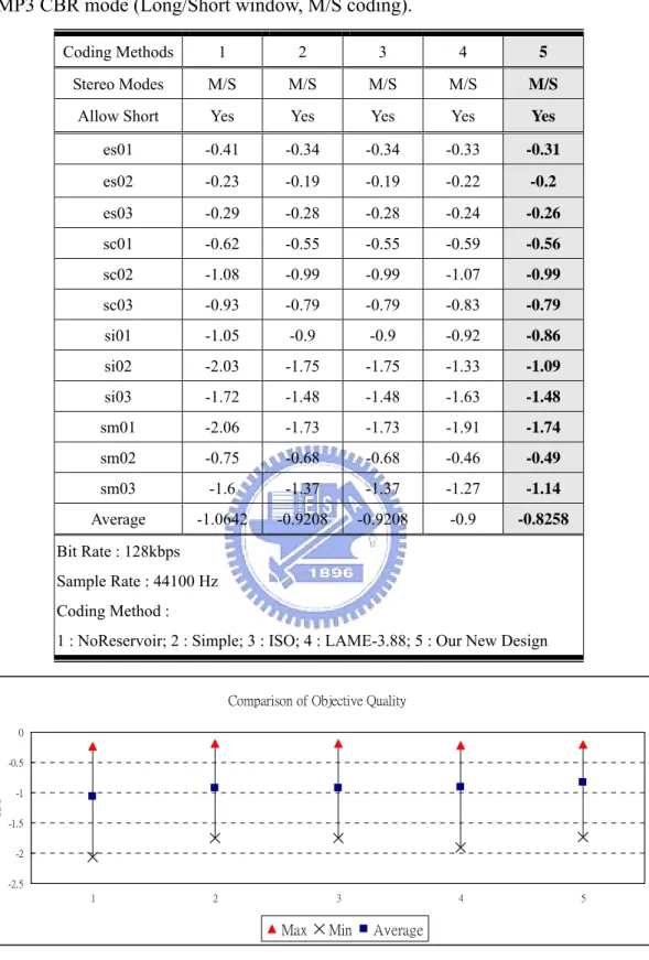
Figure 35: The ODG range comparison of Table 3. The top arrow represents the maximum ODG value, the down cross represents the minimum ODG value, and the middle square represents average ODG value among the twelve test tracks. ...40
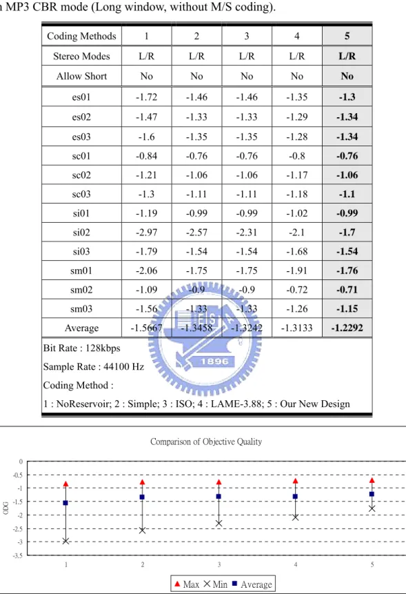
Figure 36: The ODG range comparison of Table 4. The top arrow represents the maximum ODG value, the down cross represents the minimum ODG value, and the middle square represents average ODG value among the twelve test tracks. ...41
Figure 37: The ODG range comparison of Table 5. The top arrow represents the maximum ODG value, the down cross represents the minimum ODG value, and the middle square represents average ODG value among the twelve test tracks. ...43
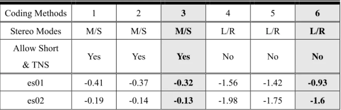
Figure 38: The ODG range comparison of Table 6. The top arrow represents the maximum ODG value, the down cross represents the minimum ODG value, and the middle square represents average ODG value among the twelve test tracks. ...44
Figure 39: The average objective quality of NCTU-MP3 CBR mode without bit reservoir and with new bit reservoir for the 16 bitstream sets in PSPLAB audio database. Bit rate: 128 kbps; Sample rate: 44100 Hz (Long/Short window, M/S coding)...51
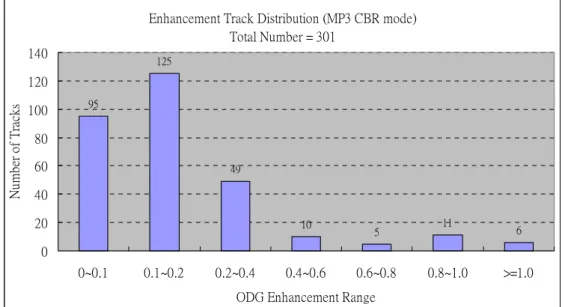
Figure 40: The enhancement tracks distribution of NCTU-MP3 CBR mode without bit reservoir and with new bit reservoir for the 16 bitstream sets in PSPLAB audio database. Bit rate: 128 kbps; Sample rate: 44100 Hz (Long/Short window, M/S coding)...51
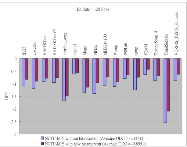
Figure 42: The average objective quality of NCTU-MP3 ABR mode
without bit reservoir and with new bit reservoir for the 16 bitstream sets in PSPLAB audio database. Bit rate: 128 kbps; Sample rate: 44100
Hz (Long/Short window, M/S coding)...52
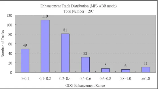
Figure 43: The enhancement tracks distribution of NCTU-MP3 ABR mode without bit reservoir and with new bit reservoir for the 16 bitstream sets in PSPLAB audio database. Bit rate: 128 kbps; Sample rate: 44100 Hz (Long/Short window, M/S coding)...53
Figure 44: The degradation tracks distribution of NCTU-MP3 ABR mode without bit reservoir and with new bit reservoir for the 16 bitstream sets in PSPLAB audio database. Bit rate: 128 kbps; Sample rate: 44100 Hz (Long/Short window, M/S coding)...53
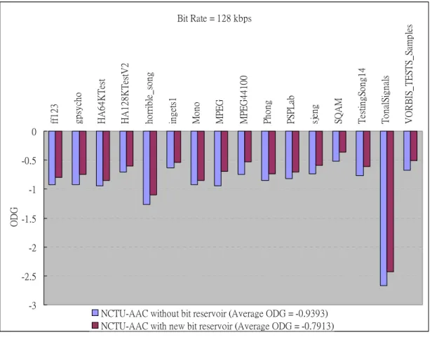
Figure 45: The average objective quality of NCTU-AAC without bit reservoir and with new bit reservoir for the 16 bitstream sets in PSPLAB audio database. Bit rate: 128 kbps; Sample rate: 44100 Hz (Long/Short window, M/S coding, TNS)...54
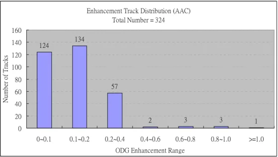
Figure 46: The enhancement tracks distribution of NCTU-AAC without bit reservoir and with new bit reservoir for the 16 bitstream sets in PSPLAB audio database. Bit rate: 128 kbps; Sample rate: 44100 Hz (Long/Short window, M/S coding, TNS)...55
Figure 47: The degradation tracks distribution of NCTU-AAC without bit reservoir and with new bit reservoir for the 16 bitstream sets in PSPLAB audio database. Bit rate: 128 kbps; Sample rate: 44100 Hz (Long/Short window, M/S coding, TNS)...55
Figure 48: The ODG range comparison of Table 11...57
Figure 49: The ODG range comparison of Table 12...57
Figure 50: The ODG range comparison of Table 13...58
Figure 51: Block diagram of SBR encoder. ...60
Figure 52: The spectrogram of an interval in input signal with the superimposed envelope time-frequency gird [5]. ...61
Figure 53: Block diagram of bit reservoir for HE-AAC. ...61
Figure 54: Natural vocal (es03). ...62
Figure 55: Complex sound (sc02). ...62
Figure 56: Transient (si02). ...63
Figure 57: Harmonic (si03)...63
Figure 58: The flow chart of bit reservoir design for HE-AAC...66
Figure 59: Objective measurements through the ODGs for three kinds of SBR demand estimator designs at 48kbps. ...68
Figure 60: Objective measurements through the ODGs for three kinds of
SBR demand estimator designs at 64kbps. ...68
Figure 61: Objective measurements through the ODGs for three kinds of
SBR demand estimator designs at 80kbps. ...68
Figure 62: Objective measurements through the ODGs for three kinds of
SBR demand estimator designs at 96kbps. ...69
Figure 63: The ODG range comparison of Table 15. The top arrow
represents the maximum ODG value, the down cross represents the minimum ODG value, and the middle square represents average ODG value among the twelve test tracks. ...70
Figure 64: The average objective quality of NCTU-HEAAC without bit
reservoir and with new bit reservoir for the 16 bitstream sets in PSPLAB audio database. Bit rate: 48 kbps; Sample rate: 44100 Hz (Long/Short window, M/S coding, TNS)...72
Figure 65: The average objective quality of NCTU-HEAAC without bit
reservoir and with new bit reservoir for the 16 bitstream sets in PSPLAB audio database. Bit rate: 64 kbps; Sample rate: 44100 Hz (Long/Short window, M/S coding, TNS)...73
Figure 66: The average objective quality of NCTU-HEAAC without bit
reservoir and with new bit reservoir for the 16 bitstream sets in PSPLAB audio database. Bit rate: 80 kbps; Sample rate: 44100 Hz (Long/Short window, M/S coding, TNS)...73
Figure 67: The average objective quality of NCTU-HEAAC without bit
reservoir and with new bit reservoir for the 16 bitstream sets in PSPLAB audio database. Bit rate: 96 kbps; Sample rate: 44100 Hz (Long/Short window, M/S coding, TNS)...73
Figure 68: The enhancement tracks distribution of NCTU-HEAAC without
bit reservoir and with new bit reservoir at different bit rates for the 16 bitstream sets in PSPLAB audio database. Sample rate: 44100 Hz (Long/Short window, M/S coding, TNS)...74
Figure 69: The degradation tracks distribution of NCTU-HEAAC without
bit reservoir and with new bit reservoir at different bit rates for the 16 bitstream sets in PSPLAB audio database. Sample rate: 44100 Hz (Long/Short window, M/S coding, TNS)...74
Figure 73: ABX dialog box of ABC/Hidden Reference Audio Comparison
Tool. ...79
Figure 74: Subjective quality evaluation of NCTU-HEAAC with and
Table List
Table 1: Idealized critical band filter bank [8]. ...8
Table 2: The twelve test tracks recommended by MPEG...38
Table 3: Objective measurements through the ODGs for different bit reservoir designs in MP3 CBR mode (Long/Short window, M/S coding). ...40
Table 4: Objective measurements through the ODGs for different bit reservoir designs in MP3 CBR mode (Long window, without M/S coding). ...41
Table 5: Objective measurements through the ODGs for different bit reservoir designs in MP3 ABR mode...42
Table 6: Objective measurements through the ODGs for different bit reservoir designs in AAC. ...43
Table 7: MP3 CBR mode parameters evaluation. ...45
Table 8: MP3 ABR mode parameters evaluation. ...46
Table 9: AAC parameters evaluation...48
Table 10: The PSPLAB audio database...49
Table 11: Objective quality comparison for MP3 CBR mode at different bit rates...56
Table 12: Objective quality comparison for MP3 ABR mode at different bit rates...57
Table 13: Objective quality comparison for AAC at different bit rates. ...58
Table 14: The minimum, maximum, average, and standard deviation of bits usage at 80 kbps. The “Minimum” and “Maximum”, “Average”, and “Standard Deviation” columns denote respectively the minimum, the maximum bits, the average bits, and the standard deviation used in the SBR encoder among all the frames in the correspondent track. The percentage in each the above category column is the bit percentage for the budget in a frame at bit rate 80 kbps...63
Table 15: Objective measurements through the ODGs for different bit
Chapter 1
Introduction
Current perceptual audio encoders like MPEG-1 Layer 3 (MP3) [1] and MPEG-4 Advanced Audio Coding (AAC) [2] has included a mechanism referred to as the bit reservoir to control the bits variation among frames. The mechanism provides the space to loan or deposit bits to control the audio quality under a bit rate constraint.
The general perceptual encoders can be considered in Figure 1. The audio signal is segmented into frames for encoding. The bit allocation module assigns the available bits provided by the bit reservoir to quantize bands according to the information from the psychoacoustic models. The bit reservoir deciding the dynamic of the available bits among frames is the quality buffer avoiding the severe quality degradation from critical frames. Time/Frequency Transform Stereo Transform Quantization VL Coding Audio Signals Packing Bit Allocation Psychoacoustic
models Bit Reservoir
Output Bit Stream
Figure 1: General Perceptual encoder.
The explicit bit reservoir in MP3 or the implicit bit reservoir in AAC have been used to efficiently maintain the frame bits and quality during varying audio contents such as attack, critical tracks, and silence. The bit reservoir design can be considered from the bit demand to compress the basic time frame in a track and the bit budget to regulate the consumed bits. The methods of bit reservoir can be classified into demand-driven method and budget-driven method. Demand-driven approach determines the required bits according to the audio contents while budget-driven one allocates bits according to the bit budgets accumulated in the bit reservoir.
budget according to the codec protocol and preferred scenario. The codec protocols affect the buffering size and resolution of the bit deposit and loan. On the preferred scenario, there are in general three cases: the constant bit rate (CBR), the variable bit rate (VBR), and the average bit rate (ABR). The CBR allows very limited bit variation in consecutive frames. The VBR in general have no regulation on the bit rates. The ABR allow the constant bit rates over a time period longer than several time-frames. The bit reservoir presented in this thesis can adjust the bit dynamic to efficiently maintain the audio quality for the CBR and the ABR.
In order to achieve high audio quality at bit rates lower than 96 kbps, High Efficiency AAC (HE-AAC) is proposed. HE-AAC is the extension of the conventional AAC codec by supporting the Spectral Band Replication (SBR) module [3][4][5][6]. The block diagram of the HE-AAC is illustrated in Figure 2. The audio signal is fed into the filterbank and split into high frequency signal sh(n) and low
frequency signal sl(n) through a filterbank. The low frequency signal sl(n) is half the
sampling rate of the original signal. The high frequency signal sh(n) is reconstructed
through the band replication technique from the low frequency signal sl(n). The
replication parameters are used to keep the reconstructed high frequency bands perceptually similar to the original high frequency bands. The bit reservoir finds the suitable bit distribution between the AAC encoder and SBR encoder according to the signal contents and the available bit budget.
Figure 2: Block diagram of HE-AAC encoder.
The bit reservoir design in AAC should be extended to HE-AAC. On the bit allocation for the AAC encoder and SBR encoder, the problem leads to a closely dependent issue. The SBR, which reconstructs the high frequency signal from the low frequency signal encoded, needs to check the AAC encoding results to predict the bit required. However, the AAC also need to know the bit consumed by SBR to efficiently encode the signals based on the available bits. Furthermore, the bit reservoir should control the quality among frames with regulation on the bit variation.
Although this kind of deadlock or interdependent issue can be approached through an iterative manner, the complexity would increases tremendously due to the inherent complexity in AAC encoder and SBR encoder. This thesis proposes a single iteration approach on the bit reservoir. Based on the demand estimator and budget regulator, we design a SBR demand estimator through a recurrent mechanism. Also, on the budget regulator, we modify the budget regulator that was used in AAC to be the one for both AAC and SBR.
This thesis is organized as follows: Chapter 2 introduces the fundamental knowledge of psychoacoustic model. Chapter 3 introduces the related bit reservoir design in current audio codec. Chapter 4 presents an efficient bit reservoir design for MP3 and AAC through demand estimator and budget regulator. Chapter 5 extends the bit reservoir design to HE-AAC through demand estimator of SBR and global budget regulator. Both subjective and objective measurements are conducted to verify the audio quality and efficiency of our bit reservoir design in Chapter 4 and Chapter 5. The objective test is based on the recommendation system by ITU-R Task Group 10/4. Chapter 6 gives a conclusion on this thesis.
Chapter 2
Backgrounds
This chapter introduces some fundamental background knowledge of the perceptual audio coding. The psychoacoustic model for optimizing coding efficiency and quality is described first. Some psychoacoustic phenomena and measurements are shown in this chapter.
2.1 Psychoacoustic Model
The objective of perceptual audio coding is to achieve transparent audio quality under bit rate constraint. The psychoacoustic model derives the masking thresholds that quantify the maximum amount of coding distortion without introducing audible artifacts from human auditory system. Therefore, the psychoacoustic model allows the coding algorithms and quantization to exploit perceptual irrelevancies. Irrelevant information is identified during signal analysis by incorporating into several psychoacoustic principles including absolute hearing thresholds, critical band analysis, simultaneous masking, the spread of masking along the basilar membrane, and temporal masking. Furthermore, the theory of perceptual entropy [7], which combines these psychoacoustic notions above with basic properties of signal quantization, is proposed. It is a quantitative estimate for transparent audio signal compression.
2.1.1 Absolute Threshold of Hearing
The absolute threshold of hearing, or threshold in quiet, represents the minimum amount of sound level at given frequency to be detected by a listener in a noiseless environment. The absolute threshold is typically expressed in terms of dB SPL, which is a standard metric for quantifying the intensity of an acoustical stimulus [8]. Through the information of absolute threshold, the quantization noise lower than this threshold level would not be perceived by human hearing so some minor details can be ignored during coding process without introducing audio distortion. In general, the threshold stimulus is measured by tuning the sound pressure level of a test tone whose frequency is slowly sweeping from low to high values to the testing listeners. Fletcher [9] reported the frequency dependence of this threshold. The result is close to the
zigzag curve as shown in Figure 3. By connecting the top and bottom points in the zigzag graph, the average of these two curves could be used to evaluate the absolute threshold of hearing.
Figure 3: Experiment result of absolute threshold of hearing [9].
Terhardt [10] proposed a well approximated nonlinear function: 4 3 ) 3 . 3 1000 *( 6 . 0 8 . 0 ) 1000 ( * 10 * 5 . 6 ) 1000 ( * 64 . 3 ) ( 2 f e f f T f q − − − − − + = (dB SPL), (1)
where Tq(f) could be deemed the maximum allowable energy level for coding
distortion applying to audio coding. The graph of the frequency dependent function above can be depicted as Figure 4.
Figure 4: The absolute threshold of hearing in quiet.
playback levels; hence the curve is often referenced to the coding system by equating the lowest point (i.e., near 4 kHz) to the energy in ±1 bit of signal amplitude [11].
2.2.2 Critical Bands
The absolute threshold of hearing shapes the basic coding distortion spectrum. However, it is not clear and definite understanding in the coding context. It is necessary to exploit the human hearing model to get maximum coding gain. The structure of human ear is shown in Figure 5. The function of outer ear is to collect sound energy and to transmit this energy through the outer ear canal to the eardrum. The eardrum that is firmly attached to the malleus operates over a wide frequency range as a pressure receiver. The motions of the eardrum are transmitted to the stapes by the middle ear ossicles named malleus, incus, and stapes. The stapes, together with a ring-shaped membrane call the oval window, forms the entrance to the inner ear. The inner ear, cochlea, is shaped like a snail and is embedded in the extremely hard temporal bone. When the oval window receives the excitation from mechanical vibrations, the cochlea structure induces traveling waves along the length of the basilar membrane. The traveling waves generate peak responses at frequency-specific membrane positions, and different neural receptors are effectively tuned to different frequency bands according to their locations. Therefore, the cochlea where the frequency-to-plane transformation takes place can be assumed as a bank of highly overlapping band pass filters [9]. These band pass filters is called the critical bands and its frequency dependent bandwidth is so called “critical bandwidth.”
Figure 5: The structure of human ear [8].
The critical bandwidth measurement experiments are shown in Figure 6. Figure 6 (a) and (c) show that the detection threshold for a narrow-band noise source presented
between two masking tones. The threshold remains constant as long as the frequency separation between the two masking tones remains within a critical bandwidth. Beyond this bandwidth, it drops off rapidly. An analogous experiment with reverse masker and maskee is shown in Figure 6 (b) and (d).
Figure 6: Critical bandwidth measurement: (a) and (c) detection threshold decreases
as masking tones transition from auditory filter passband into stopband; (b) and (d) the same interpretation with roles reversed [11].
The critical bandwidth can be conveniently approximated [8] by 69 . 0 2] ) 1000 ( 4 . 1 1 [ 75 25 f f = + + ∆ (Hz). (2)
The critical bandwidth is narrower in low frequency region and wider in high frequency region. The curve of critical bandwidth and the relation between frequency and critical band can be illustrated in Figure 7.
In addition, a distance of one critical band is commonly referred to as one “Bark”. The formula [8] ] ) 7500 arctan[( 5 . 3 ) 1000 76 . 0 arctan( 13 ) (f f f 2 z = + (Bark). (3)
is often used to transfer from frequency in Hertz to the Bark scale. Table 1 gives the transformation that the nonuniform Hertz spacing of the filter bank is actually uniform on Bark scale. The masking curve shapes are much easier to describe with the Bark scale notion.
Table 1: Idealized critical band filter bank [8].
Band No. Central Frequency (Hz) Bandwidth (Hz) Band No. Central Frequency (Hz) Bandwidth (Hz) 1 50 0 – 100 14 2150 2000 – 2320 2 150 100 – 200 15 2500 2320 – 2700 3 250 200 – 300 16 2900 2700 – 3150 4 350 300 – 400 17 3400 3150 – 3700 5 450 400 – 510 18 4000 3700 – 4400 6 570 510 – 630 19 4800 4400 – 5300 7 700 630 – 770 20 5800 5300 – 6400 8 840 770 – 920 21 7000 6400 – 7700 9 1000 920 – 1080 22 8500 7700 – 9500 10 1170 1080 – 1270 23 10500 9500 – 12000 11 1370 1270 – 1480 24 13500 12000 – 15500 12 1600 1480 – 1720 25 19500 15500 - 13 1850 1720 – 2000 2.2.3 Masking Effects
Masking effect is the phenomenon that one sound is inaudible because of the existence of another sound at the same time. It is an important reference for perceptual audio encoder designers to optimize the bit allocation strategy for input signals. If one sound tends to be masked by other sounds, the audio encoder could allocate most bits to the most audible sound and allocate little bits to the insensitive one. However, the relation between masker and maskee is complicated, and it is difficult to exactly analyze the masking effect within them. In general, the masking effects could be discussed from two categories: simultaneous masking (spectral
masking) and nonsimultaneous masking (temporal masking). 2.2.3.1 Simultaneous masking
The simultaneous masking is that the existence of a strong tone or noise masker creates excitation of sufficient strength on the basilar membrane at the critical band location to block effective detection of a weaker signal. This phenomenon in spectral domain is shown in Figure 8. This figure illustrates the masker with strong SPL masks the other weak signals at nearby frequencies. The masking threshold indicates the lowest sound level that can be heard. Therefore, we can focus on the significant components and ignore those unperceived ones.
Figure 8: Example of simultaneous masking.
2.2.3.1 Nonsimultaneous masking
Nonsimultaneous masking, or temporal masking, as shown in Figure 9 is different to simultaneous masking in occurrence of maskee. There are two types of temporal masking: pre-masking and post-masking. Pre-masking appears before the onset of the masker; post-masking appears after the masker is vanished.
Figure 9: Example of nonsimultaneous masking [8].
The statement of pre-masking is not well comprehensible since it occurs prior to the masker is trigger. The duration of pre-masking lasts 50~60 ms but only a few milliseconds preceding the masker are effective. Pre-masking is an important design issue for pre-echo problem. It has been utilized in conjunction with adaptive block switching to compensate for pre-echo distortions in several audio coding. With referring to post-masking, it presents a momentary masking after the masker and stronger masking effect than pre-masking. Post-masking can sustain more than 100 ms after the maker removal. The duration of post-masking depends on the strength, duration, and relative frequency of masker [8].
2.2 Psychoacoustic Model in MP3 and AAC
There are two psychoacoustic models presented in [1]. The calculation of the psychoacoustic parameters can be done either with Psychoacoustic Model I or Psychoacoustic Model II. Typically, Model I is applied to MPEG-1 Layer I and II, and Model II to MPEG-1 Layer III, MPEG-2 AAC, and MPEG-4 AAC. The process of psychoacoustic model is mainly to receive the time representation of the signal content over a certain time interval and the corresponding outputs are the signal-to-mask ratio (SMR) for every frequency partition in coders. Based on SMR, the noise shaping allowance and bit allocation are determined for each band in input signals. In this section we only pay attention to Psychoacoustic Model II because Model I is not the main policy adopted in MP3 and AAC encoder design.
A block diagram of Model II is shown in Figure 10. At the first stage, analysis stage, the input data is applied to a Hanning-windowed FFT. The outputs of FFT are grouped into “threshold calculation partitions” which are roughly 1/3 of a critical band or one FFT line wide. The following procedures are divided into two branches. One branch uses the predicted magnitude and phase for unpredictability measure
calculation. The unpredictability is convolved with a spreading function to estimate the tonality index. The property of tonality is that high unpredictability approaching to 0 while low unpredictability approaching to 1. In the other one branch, the partitioned energies are also applying the same spreading function. With the tonality, we can use the noise masking tone (NMT) and tone masking noise (TMN) effects to evaluate the signal-to-noise ratio (SNR). Finally, the actual SMR is derived from SNR and the renormalized signal energies with spreading function.
FFT Unpredictability Levels Signal Levels Spread Unpredictability Levels Tonality Indices Masking Levels SMR per subband Spread Signal Levels Input Signal Perceptual Entropy
Figure 10: Block diagram of MPEG Psychoacoustic Model II [12].
The precise steps for masking calculation in Psychoacoustic Model II are depicted in Figure 11. We only point out the main function in each step. The details are described in [1] and [2]. r(w) and f(w) represent the magnitude and phase components. c(w) represents the unpredictability measure.
Figure 11: Flow chart of MPEG Psychoacoustic Model II.
2.3 Perceptual Entropy
Johnston [7][13] defined the perceptual entropy (PE) as a measure of perceptually relevant information contained in audio signals. PE combines the psychoacoustic masking with signal quantization principles to represent theoretical bits requirement for transparent audio coding. The signal is first windowed and transformed to the frequency domain. The masking threshold is then obtained by perceptual rules. Finally, the number of bits required to quantize the spectrum without injecting any perceptual difference with respect to the original signal is determined. The estimation process of PE is accomplished as follows:
First, it is assumed that the quantization noise σn associated with a uniform quantizer with step size ∆ is given by
12 2 2 = ∆
n
σ . (4)
Reconstruct samples of input signals
Calculate the complex spectrum of input signals
Estimate predicted value of r(w) and f(w)
Calculate the unpredictability measure c(w)
Calculate energy and unpredictability in threshold calculation partition band
Convolve partitioned energy and unpredictability with spreading function
Tonality index calculation
Calculate required SNR in each partition band
Calculate the power ratio
Calculate actual energy threshold
Pre-echo control Absolute threshold in quiet
Then the masking power per spectral line is calculated as i i k T , (5)
where Ti is the psychoacoustic masking threshold and ki is the number of spectral
lines in critical band i. Since the real and imaginary parts of the spectrum are quantized independently, the energy at each frequency must be divided by 2. Hence the masking power per real and imaginary components is
i i
k T
2 . (6)
Next we want that the quantization noise per component can be lower than the masking capacity. It means
i i i k T * 2 12 2 ≤ ∆ , (7)
and the step size ∆i is derived from
2 1 * 6 ⎟⎟ ⎠ ⎞ ⎜⎜ ⎝ ⎛ ≤ ∆ i i i k T . (8)
Now, the quantizer levels Ni to represent quantized spectral lines are determined by
⎟⎟ ⎠ ⎞ ⎜⎜ ⎝ ⎛ ∆ = i i NRe(ω) nint Re(ω) , (9) and ⎟⎟ ⎠ ⎞ ⎜⎜ ⎝ ⎛ ∆ = i i NIm(ω) nint Im(ω) , (10) where ω represents each spectral line in critical band i, nint is a function that returns the nearest integer to its argument, and | | denotes the absolute value function. With the level information, the number of bits required for per band i are
) 1 ) ( * 2 ( log ) ( Re 2 Re ω = ω + i i N b , (11) and ) 1 ) ( * 2 ( log ) ( Im 2 Im ω = ω + i i N b . (12)
) 1 / * 6 ) Im( int * 2 ( log ) 1 / * 6 ) Re( int * 2 ( log ) ( 2 2 Im Re + ⎟ ⎟ ⎠ ⎞ ⎜ ⎜ ⎝ ⎛ + + ⎟ ⎟ ⎠ ⎞ ⎜ ⎜ ⎝ ⎛ = + =
∑
∑
= = i i bh bl i i bh bl i i i k T n k T n b b PE i i i i ω ω ω ω , (13) (14) where bl and i bh are lower and upper bounds of band i. iChapter 3
Bit Reservoir Design in Current
Audio Codec
This chapter reviews the bit reservoir schemes in current codec standards and audio encoders to illustrate the fundamentals of bit reservoir design and to provide reference materials for comparing with our proposed design.
3.1 Bit Reservoir Schemes in MP3 Codec
MPEG-1 Layer III (MP3) uses a so-called bit reservoir to make up for temporary shortage of bits required for encoding. If a frame is easy to code then the some of the bits can be saved in the reservoir. If a frame is difficult to compress, some additional bits can be allocated to the frame. Through this mechanism, the reservoir can control the audio frame quality without direct limitation to the bit regulation.
3.1.1 Frame Format
The bitstream format of MP3 [1] is shown in Figure 12. The length of Header is always 4 bytes long; the length of side information is 17 bytes in mono mode and 32 bytes in stereo mode. The distance between adjacent frame headers is determined by bit_rate_index in Header. Once the value of bit_rate_index in current frame is extracted, the position of next frame header can be derived immediately.
Figure 12: Bitstream format of MPEG-1 Layer III [1].
The bit reservoir technique is realized by the dynamic data allocation of MP3. It is implemented by a 9-bit pointer (main_data_begin), which indicates the location of the starting byte of the audio data (main_data) for that frame, in side information. The frame structure is shown in Figure 13. With the assistance of main_data_begin pointer, the Frame 3 with much more demand can utilize the space of Frame 2 to achieve better quality without breaking bit rate restriction.
Frame 1 Frame 2 Frame 3
main_data_begin 1
Frame 4
sync sync sync sync side info 1 side info 2 side info 3 side info 4
main_data 4 main_data 3
main_data 2 main_data 1
main_data_begin 2 main_data_begin 3 main_data_begin 4
Figure 13: Example of MP3 frame structure [1].
The main_data_begin pointer also determines the maximum bit reservoir size in MP3. The maximum amount of accumulated bits is calculated by
4096 2 * 8 size reservoir bit Maximum = 9 = (bits) (15) The exceed bits will be padded to maintain bit rate constraint while the bit reservoir overflows.
3.1.2 Bit Rate Scenario
On the preferred scenario, there are three cases: the constant bit rate (CBR), the variable bit rate (VBR), and the average bit rate (ABR). Coding at a constant perceptual quality generally leads to a variable rate coding like VBR. The VBR in general has no regulation on bit rates. Conversely, coding at a constant bit rate like CBR will usually result in a time-dependent coding quality depending on segments of input signal. The CBR allows very limited bit variation in consecutive frames. Both concepts can be combined advantageously by using ABR. ABR allows the constant bit rate over a time period longer than several time-frames and attains constant output quality over times. Therefore, our efficient bit reservoir design for MP3 presented in this thesis mainly focuses on CBR mode and ABR mode.
The implementation of CBR mode in MP3 is achieved by fixed bit_rate_index setting. Hence the maximum size of bit reservoir is 4096 bits as calculate in (15). In ABR mode, the bit_rate_index can vary between frames as long as the bit rate on average over a long time satisfies the desired bit rate request. For this reason, the limitation of physical bit reservoir size can be freed. An abstract bit reservoir with larger size, which is implemented by adjusting bit_rate_index dynamically, is used to regulate bit rate and obtain better audio quality. The details are shown in later chapters in this thesis.
3.1.3 Recommended Scheme in Standard
The MPEG draft [1] recommends a scheme for bit reservoir design. The numbers of bits, which are made available for the main_data are derived from the actual estimated threshold (the PE as calculated by the psychoacoustic model), the average number of bits (mean_bits) and the actual content of the bit reservoir. The number of bytes in the bit reservoir is given by main_data_begin. The actual rules for controlling bit reservoir in [1] are given in Figure 14.
R > R_MAX * 0.8 extra_bits = R - R_MAX * 0.8 more_bits > 100 extra_bits += max(more_bits, R * 0.6) Yes No Yes No
The variables in Figure 14 are defined as follow: R current reservoir size;
R_MAX maximum allowable reservoir size; more_bits derived from
bits mean PE
bits
more_ =3.1* − _ ; (16)
PE perceptual entropy calculated by the psychoacoustic model;
max() function that return the maximum value between arguments; mean_bits average bits of one frame derived from desired bit rate; allocation_bits allocated bits for quantization.
After the actual loops computations have been completed, the number of bytes not used for main_data is added to the bit reservoir. If the number of bytes accumulated in the bit reservoir exceeds the maximum allowable content, stuffing bits are written to the bitstream and the content of the bit reservoir is adjusted accordingly. This scheme only considers the reservoir size variation (budget size) and roughly estimates the demand. It may encounter quality risks while applying to different bit rate request.
3.1.4 Scheme in LAME 3.88
LAME 3.88 [14] is currently a popular MP3 encoder. The bit reservoir control scheme in LAME 3.88 is depicted in Figure 15. The variables in Figure 15 are defined as follows:
R current reservoir size;
R_MAX maximum allowable reservoir size;
PE perceptual entropy calculated by the psychoacoustic model;
ch channel index;
mean_bits average bits of one frame derived from desired bit rate; add_bits temporary variable in reservoir control steps.
The allocated bits per channel, allocation_bits[ch], is derived by
] [ _ ] [ _ ] [
_bits ch mean bits ch add bits ch
allocation = + . (17)
In the mechanism, there are some heuristic number like 750 and 1.4, this number will lead to variation on the different bit rates and sample rates. Furthermore, there is no deposit mechanism for bit reservoir in addition to the silence frames. Hence in most situations, there is no bit deposited in the reservoir to regulate the bit demand from critical audio frames.
R > R_MAX * 0.9
add_bits = R - R_MAX * 0.9 add_bits = 0
R > R_MAX * 0.6
extra_bits = R_MAX * 0.6 extra_bits = R
extra_bits -= add_bits Yes No Yes No extra_bits < 0 extra_bits = 0 add_bits[ch] = (PE[ch] - 750) / 1.4 add_bits[ch] > mean_bits * 0.75 Yes No add_bits[ch] = mean_bits * 0.75 add_bits[ch] < 0 add_bits[ch] = 0 Yes No add_bits[0] + add_bits[1] > extra_bits Yes No
add_bits[ch] = extra_bits * (add_bits[ch]/ (add_bits[0]+ add_bits[1]))
Yes
3.2 Bit Reservoir Schemes in AAC
AAC follows the same basic paradigm as MP3 (high frequency resolution filterbank, non-uniform quantization, Huffman coding), but includes a lot of new coding tools to improve the coding efficiency. Also, with the flexible bitstream format, AAC can achieve a high bits variation among frames to control the frame quality and various bit rate scenario.
3.2.1 Bitstream Format
The MPEG-4 AAC [2] system has a very flexible bitstream syntax. There are two parts in AAC bitstream: Audio Data Interchange Format (ADIF) and Audio Data Transport Stream (ADTS). The type of each audio format is shown in Figure 16 and Figure 17. ADIF is not used in the on-line network environment because that is the storage mass, so playing is impossible at some point of bitstream. ADTS is possible playing at the network environment because there are syncword, CRC and frame length information in bitsream. Therefore, we focus on ADTS format as our research domain. adif_id(32) [0x41444946 =“ADIF”] co pyr ight_id_present(1) copyright_id(72) 8+64=72 copyright_id(8) +copyright_number(64) original_copy(1) home(1) bitstream_type(1) bitrate(23) num_program_config_ E lements(4) adif_buff er_f ullness
Program_config_ elements(20) adif_buff
er_f
ullness
Program_config_ elements(20)
adif_header byte_alignment raw_data_stream
adts_fixed_header adts_va riable_header adts_ erro r_ch eck raw_data_block byte_al ignment syncword(12) [1111 1111 1111] ID(1) ‘1’ la yer( 2) ‘00 ’ pr ote ction_abse nt(1 ) pr of ile(2 ) sa mpling_frequ en cy_ ind ex (4) pr iva te_bit (1) chann
el_configuration(3) original/copy(1) home(1)
cop yr igh t_id en tifi cat ion _bi t(1) fra m e_len gt h( 13) copyright_identification_ start(1) adts_buffer_fullness(11) nu mber_o f_r aw_d at a_ blocks_in_frame(2) CRC_ ch ec k(16)
Figure 17: ADTS bitstream [2].
Since the AAC system has a data buffer that permits its instantaneous data rate to vary as required by the audio signal, the length of each frame is not constant. In this respect the AAC bitstream uses a variable rate headers that are byte-aligned so as to permit editing of bitstreams at any frame boundary. It is the main difference with MP3 discussing in section 3.1.1. Because the distance between headers is no longer fixed, the bitstream element, syncword, is used for searching header position. The syncword is composed of bit string ‘1111 1111 1111.’ Once the decoder meets up syncword in bitstream, the position of header is derived quickly for decoding process.
The maximum bit reservoir size in AAC is limited by decoder input buffer size while in MP3 is determined by main_data_begin pointer. The maximum bit reservoir size for constant rate can be calculated by subtracting the mean number of bits from the minimum decoder input buffer size. Such as
bits mean bits channel ma reservoir bit max_ _ = x_ _ *2− _ . (18)
where max_bit_reservoir is the maximum bit reservoir size, max_channel_bits is the maximum number of bits per channel that is 6144, and mean_bits is the average number of bits per frame. For variable bit rate the encoder must operate in a way that the input buffer requirements do not exceed the minimum decoder input buffer.
reservoir control not only implies on short-term frames but also implies on whole track for bit rate control. The details are shown in later chapters in this thesis.
3.2.2 Recommended Schemes in Standard
The paper [2] provides a rough bit reservoir control method. Bits are saved to the bit reservoir when the bits are fewer than the mean_bits of one frame. If the reservoir is full, unused bits have to be encoded in the bitstream as fill-bits. The maximum amount of bits available for a frame is the sum of mean_bits and bits saved in the bit reservoir. The number of bits that should be used for encoding a frame depends on the maximum available bits and more_bits value, which is calculated by
) _ f _ _ ( _
_bits bit allocation mean bits side in o bits
more = − − . (19)
where bit_allocation is derived from psychoacoustic model, side_info_bits is bits used for side information. The actual rule is given in Figure 18.
more_bits > 0
available_bits = average_bits + min(more_bits, bitres_bits)
available_bits = average_bits + max(more_bits, bitres_bits - max_res_bits)
Y
N
Figure 18: Flow chart of bit reservoir control in [2].
The variables in Figure 18 are defined as follow: available_bits bits used for quantization;
average_bits the mean number of bits per frame derived from desired bit rate; min() function that returns the minimum value within arguments; max() function that returns the maximum value within arguments; bitres_bits bits saved in bit reservoir;
max_res_bits maximum bit reservoir size calculated by (18).
3.2.3 Schemes in FAAC 1.24
seems to have no bit reservoir control design in FAAC except the check of input buffer restriction. The only relative part is the function “MaxBitresSize” that is used for stuffing. Hence we have no any other discussion about FAAC here.
3.3 Bit Reservoir Schemes in HE-AAC
HE-AAC [3] is the combination of conventional AAC codec and Spectral Band Replication (SBR) module to achieve high audio quality at low bit rates. There are no definite statements concerning bit reservoir design for HE-AAC in [3]. Current limited literature seems to have no relative bit reservoir design in HE-AAC. We propose a novel design [16] and state it explicitly in this thesis.
3.3.1 Bitstream Overview
The bitstream of HE-AAC shown in Figure 19 is form by AAC frame and SBR frame. The decoder will identify the content of bitstream element to determine whether it is sycnword for next AAC frame header or header flag for SBR frame. The decoding process of SBR part is independent of AAC part. Hence the bits distribution between AAC and SBR in HE-AAC frame leads to dependent issue. How to allocate bits properly would affect the audio quality and bit rate control.
AAC header AAC main_data
syncword SBR extension data element
header flag main, tuning grid, dtdf, ctrl envelope and noise floor data etc
Side_info Raw data
Data Header
header flag
Figure 19: Bitstream organization of HE-AAC [3].
3.3.2 Schemes in 3GPP
The 3rd Generation Partnership Project (3GPP) provides a reference code for HE-AAC [17]. The flow chart of 3GPP is given in Figure 20. There is a bit reservoir
appropriately adjusted. The masking threshold to be adjusted is different from the one calculated by psychoacoustic model. The psychoacoustic model calculates the idea masking for human hearing. The adjusted masking is used to estimate the scale factor for quantization later. So the available bits for AAC part are derived from Usable_bits, which is calculated by subtracting SBR bits from mean bits of HE-AAC, and Reservoir_bits. Although this strategy in 3GPP maintains bit rate constrain but comes up against quality degradation in AAC part.
Psychoacoustic model Desired_PE Usable_bits Transform Corresponding_PE = Bits2pe(Usable_bits) Corresponding_PE' < Desired_PE BitFactor calculation (Corresponding_PE'= Corresponding_PE * BitFactor) PE correction (Corresponding_PE'*= CorrectionFactor) Usable_Bits is not enough Usable_Bits is enough Adjust masking to
get new Desired_PE
Allocate Available_bits (Available_bits = Usable_bits + Reservoir_bits) to each channel according to ratio of (PE_ch / PE_total)
Y N
Chapter 4
Efficient Bit Reservoir for MP3 and
AAC
The bit reservoir deposits bits from “easy” frames and loans bits for “difficult” frames. The efficiency of bit reservoir depends on the accuracy to predict the demand bits with consideration to the bit rates, accumulated bits, audio contents, allowable bit-variation range, allowable bit-variation resolution, and tools used in the encoder. These factors are jointly considered through two modules: demand estimator and budget regulator. The demand estimator will take care of the factors like bit rates and bit-quality dynamics. Based on the demand bits, the budget regulator will decide the available bits from the tools used and the allowable range or resolution of bit variation. As mentioned in Chapter 3, there is limited information on the detailed bit reservoir implementation in current literature. However, the basic approach is to predict demand bits through the perceptual entropy and budget control through the fullness of bit reservoir. The variation with the bit rates and the statistics of the quality over frames is usually not well considered. On the other budget part, the loan range and the resolution are two spaces that can be extended in addition to the fullness control. Therefore, this chapter will present an efficient bit reservoir design based on the demand estimator and the budget regulator for MP3 and AAC.
4.1 Allocation Entropy
Johnston [7][13] defined the perceptual entropy (PE) to reflect the minimum bits required for transparent quality. The PE is defined as
) 1 ( log * 10 + = i i i W SMR PE , (20)
where Wi is the number of spectrum lines in partition band i. The partition band has a
bandwidth proportional to the critical bandwidth. The signal-to-masking ratio SMRi is
where Ei and Mi are the spectrum energy and masking threshold in partition band i.
Except the general perceptual entropy, there is another perceptual criterion, allocation entropy (AE) [18]. The PE does not reflect the bits required for the case where the transparent quality is not achievable under limited bit rates. For audio coding, the main issue is the tradeoff between bits-constrain and quality instead of achieving transparent quality. The AE could well reflect the bits required to have the graceful degradation and have put into consideration the bandwidth proportional noise-shaping criterion [19]. To derive the AE, we modify the SMRi in (21) as SMR’q:
⎪ ⎩ ⎪ ⎨ ⎧ < ≥ = ) * ( , 0 ) * ( , * ' q i i q q q q q q q B M E if B M E if B M E SMR , (22)
where q is the index of quantization band and the effective bandwidth Bq defined in
[19] is illustrated in Figure 21 and Figure 22. Therefore, the definition of AE in each band can be described as
) 1 ' ( log * 10 + = q q q W SMR AE , (23)
where Wq is the number of spectrum lines in quantization band q.
If the noise is higher than masking threshold, a noise proportional to effective bandwidth is the suitable bit allocation criterion for optimum graceful degradation according to [19]. The effective bandwidth is derived from the critical band with bandwidth about one-third to one-forth of the critical bandwidth. In general, the higher spectrum bands often have wider effective bandwidth and should have a higher noise shape. Also, the AE is evaluated with the unit of the scale factor bands to match directly the units in quantization and encoding process.
Effective Bandwidth B(q) in MP3 0 5 10 15 20 1 3 5 7 9 11 13 15 17 19 21 Quantization Band (q) B(q)
Figure 21: Effective bandwidth for MP3 (Long Window, Sample Rate: 44.1 KHz)
Effective Bandwidth B(q) in AAC 0 5 10 15 20 1 4 7 10 13 16 19 22 25 28 31 34 37 40 43 46 49 Quantization Band (q) B( q)
Figure 22: Effective bandwidth for AAC (Long Window, Sample Rate: 44.1 KHz)
[19].
Since the granule in MP3 and the frame in AAC is the basic coding unit, we need to sum up the values of AE in each quantization band. The bits required for either the granule or the frame can be obtained from
∑∑
=∑∑
+ = ch q chq ch q chq chq SMR W AE f AE( ) , , *log10( ' , 1), (24)where ch is the channel index, q is the quantization band index, Wch,q is the number of
spectrum lines in quantization band q of channel ch, SMR’ch,q is the signal-to-masking
ratio as shown in (22) for quantization band q of channel ch, and f is the frame or granule index. AE(f) represents the bits required for the frame to have a specified quality.
In order to illustrate that AE is the representative of bits required for variable signals, we list some tracks with its corresponding spectrogram and AE as examples. These tracks shown in Figure 23 to Figure 26 are chosen from Table 2. From the results in Figure 23-Figure 26, the AE definitely indicates the transient of signals. Based on this information, the demand estimator design in later section is appropriate to evaluate the bits required for each frame.
AE Hz
Frame
Figure 23: The spectrogram (top) and the values of AE (bottom) of natural vocal
(es03).
AE Hz
Frame
Figure 24: The spectrogram (top) and the values of AE (bottom) of complex sound
(sc02).
AE Hz
Frame
AE Hz
Frame
Figure 26: The spectrogram (top) and the values of AE (bottom) of harmonic (si03).
4.2 Demand Estimator
The responsibility for demand estimator is to actively allocate bits among frames instead of passively consumes accumulated bits. The demand estimator adaptively predicts the bits required for a frame according to the audio content. The proposed idea based on the allocation entropy is to predict demand bits through average in the past and demand ratio calculation. The demand estimator will also take care of the factors such as bit rates and bit-quality dynamics.
4.2.1 AE Average
In addition to AE, which represents the requirement for a frame, we should have the average demands aligned to the average bit rates to control the average quality. The average demand AEaverage can be estimated through the average over past N
frames: UBound f AE LBound for N f AE AE N f average = < <
∑
= ) ( , ) ( 1 , (25)where LBound is the lower bound of AE and UBound is the upper bound of AE. The boundary constraint comes from the definition of masking threshold in SMR’q
calculation as shown in (22). The masking threshold Mq for quantization band q is
defined as )) * _ , min( , max(qthr T T l repelev Mq = q q q , (26)
strong attack signal, the Mq of the Kth signal is the small value T_lq*repelev, not Tq. So
the corresponding AE of the Kth signal with strong energy will be extremely large. This kind of AE only indicates the occurrence of transient but the actual bits demand is drowned in that enormous value. In order to filter out this type of interference in AEaverage calculation, the AE(f) larger than UBound should not be put into reference
frames. The similar reason is applied on AE(f) smaller than LBound to avoid the influence from silence frames. The flow chart of detailed AEaverage calculation
processes is depicted in Figure 27. Num_AE denotes the number of processed frames. AEcur denotes the AE of current frame. Reference_Array denotes the temporary array
that stores the AEs of past frames.
Num_AE >= N N f AE AE N f average
∑
= = 1 ) ( AEcur > UBound AEcur > UBound AEcur < LBound AEcur < LBound
Do Not Put AEcur into Reference_Array
Do Not Put AEcur into Reference_Array
Put AEcur into Reference_Array
AEaverage = UBound AEaverage = AEcur
Do Not Put AEcur into Reference_Array
Do Not Put AEcur into Reference_Array
Put AEcur into Reference_Array Y N Y Y N N Y N Y N
Figure 27: Flow chart of AEaverage calculation.
4.2.2 Demand Ratio
Through the average AE, we could evaluate the demand ratio D to represent the trend of demand variation.
average average AE AE f AE f D( )= ( )− . (27)
D(f) represents the current demand over the previous N coding units. The demand ratio D(f) should be transformed into Rdemand(f) by a transform function to shape the
curve and clip the upper/lower bounds:
)) ( ( ) (f D f Rdemand =η . (28)
The three η(⋅) examples used in MP3 [20] and AAC [21] encoders are illustrated in Figure 28 to Figure 30.
4.2.2.1 Demand Curve for MP3 CBR Mode
-0.2 2.375 3.85 -1.0 -0.8 -0.2 0.55
R
demand(f)
0. 45 1.5Figure 28: Demand curve for MP3 CBR mode.
Figure 28 illustrates the transform function of demand ratio for MP3 CBR mode. The slope is small due to the limited explicit budget buffer size. The “zero-zone” from -0.2 to 0.45 in D(f) is used to neglect the slight demand variation come from the prediction accuracy based on AE and AEaverage. The saturation value of Rdemand(f) is set
to 1.5 with referring to the ratio of maximum bit rate (320 kbps) to reference bit rate (128 kbps). The lower bound of Rdemand(f) is set to -0.2 to prevent quality degradation
4.2.2.2 Demand Curve for MP3 ABR Mode 0.01 -1.0 -0.8 -0.2 -0.1 Rde mand(f) 1.5 0.6 0.25 0.6 0.5 0.25
Figure 29: Demand curve for MP3 ABR mode.
Figure 29 illustrates the transform function of demand ratio for MP3 ABR mode. ABR mode has an implicit bit reservoir in addition to the explicit bit reservoir. With such flexible reservoir budget condition, the slope could increase with demands growing. Also the zero-zone of D(f) in negative part could be stretched to tolerate much more negative demands. The saturation value of Rdemand(f) is set to 1.5 by the
same reason in CBR mode. The lower bound of Rdemand(f) could be set to -0.1 to
4.2.2.3 Demand Curve for AAC -0.66 1.2 0.5
R
demand(f)
-0.3 -0.054 0.6 1.0D(f)
-0.2Figure 30: Demand curve for AAC ABR mode.
Figure 30 illustrates the transform function of demand ratio for AAC ABR mode. The slope is constant due to the intensive tools (e.g. M/S Coding [22], Window Switch [23], TNS [24]) used. Owing to these auxiliary modules the upper bound and lower bound setting of Rdemand(f) is more conservative.
4.3 Budget Regulator
The budget regulator decides the available bits according to the preferred scenario. We define a budget ratio and adjust the budget ratio with the fullness (denoted as F) of the bit reservoir. The variable F stands for the fullness of the bit reservoir budget. The fullness F is evaluated through
MAX
S S
F = , (29)
where S is the current accumulated budget size, SMAX is the maximum allowable bit
reservoir size. SMAX is defined as
B bits mean
ABR mode. It means that the budget buffer size is allowed to be negative. We can draw bits in advance and reimburse them in near future as long as conforming to the desired bit rate. Therefore, the eq. (29) could be redefined as
⎪ ⎪ ⎩ ⎪ ⎪ ⎨ ⎧ − ≤ ≤ − > = else S S S if S S S S if F MAX MAX MAX MAX , 1 , , 1 . (31)
The fullness F should be transformed into Rbudget by a transform function to regulate
the depositing or loaning rate:
) (F
Rbudget =ϕ . (32)
The three φ(·) examples used in MP3 [20] and AAC [21] encoder are illustrated in Figure 31 to Figure 33.
4.3.1 Budget Curve for MP3 CBR Mode
1.0
0.9 Rbudget
1.05
0.6
F
Figure 31: Budget curve for MP3 CBR mode.
Figure 31 illustrates the transform function of budget regulator for MP3 CBR mode. As described in section 3.1.1, the maximum bit reservoir size in MP3 CBR mode is limited by frame format. Since the maximum reservoir size is small and inflexible, the budget regulator only gives extra bonus for granules while reservoir budget is almost full. In other words the demand estimator plays a major role for bit reservoir controlling in MP3 CBR mode.
4.3.2 Budget Curve for MP3 ABR Mode Rbudget 0.5 -0.2 -0.6 1.25 1.5 0.7 0.37 0.07 F
Figure 32: Budget curve for MP3 ABR mode.
Figure 32 illustrates the transform function of budget regulator for MP3 ABR mode. The “flat-zone” from -0.2 to 0.07 is used to eliminate the function of budget regulator while the bit reservoir is not full or deficient in order to prevent wasting budget or degrading quality. The increasing rate of Rbudget slows down when the
reservoir approaches full. The lower bound of Rbudget is set to 0.5 to refund bits and
4.3.3 Budget Curve for AAC -1.0 -0.7
R
budget 1.0 0.75 0.8 0.7 -0.5 -0.4 1.15 1.0 0. 1 0.35 0. 7 1.5F
1.375Figure 33: Budget curve for AAC ABR mode.
Figure 33 illustrates the transform function of budget regulator for AAC ABR mode. The trend is similar to that for MP3 ABR mode but with a little detailed due to adopt other auxiliary modules.
4.4 Allocated Bits Calculation
The proposed bit reservoir design not only manages accumulated bits but also determines allocated bits for each coding units based on novel concept of adaptive budget buffer size. Through the demand estimator and the budget regulator, the allocated bits for encoding units is derived from
budgt demnd mean bits R
R bits mean bits
Allocated_ = _ + * _ * , (33)
where mean_bits is derived from the desired bit rate, Rdemand comes from demand
curve, and Rbudget comes from budget curve. The Allocated_bits is used for bit
allocation and quantization later. The over estimated bits are reclaimed after quantization and feed into bit reservoir for next coding unit. There is an exception need to be noticed. If the Rdemand is smaller than zero, the Rbudget is revised to one to
avoid undesired product of Rdemand and Rbudget. The flow chart of our efficient bit