Multifractality of instantaneous normal modes at mobility edges
B. J. Huang and Ten-Ming Wu*
Institute of Physics, National Chiao-Tung University, HsinChu, Taiwan 300, Republic of China
共Received 8 July 2010; revised manuscript received 7 October 2010; published 29 November 2010兲
In terms of the multifractal analysis, we investigate the characteristics of the instantaneous normal modes 共INMs兲 at two mobility edges 共MEs兲 of a simple fluid, where the locations of the MEs in the INM spectrum were identified in a previous work关B. J. Huang and T. M. Wu,Phys. Rev. E 79, 041105共2009兲兴. The mass exponents and the singularity spectrum of the INMs are obtained by the box-size and system-size scalings under the typical average. The INM eigenvectors at a ME exhibit a multifractal nature and the multifractal INMs at each ME yield the same results in generalized fractal dimensions and singularity spectrum. Our results indicate that the singularity spectrum of the multifractal INMs agrees well with that of the Anderson model at the critical disorder. This good agreement provides numerical evidence for the universal multifractality at the localization-delocalization transition. For the multifractal INMs, the probability density function and the spatial correlation function of the squared vibrational amplitudes are also calculated. The relation between the prob-ability density function and the singularity spectrum is examined numerically, so are the relations between the critical exponents of the spatial correlation function and the mass exponents of the multifractal INMs. DOI:10.1103/PhysRevE.82.051133 PACS number共s兲: 05.40.⫺a, 05.45.Df, 63.50.⫺x, 72.15.Rn
I. INTRODUCTION
The localization-delocalization transition 共LDT兲 induced by disorder, also known as the Anderson transition, is at the forefront of physics and has been intensively studied with the model proposed by Anderson for the transport of noninter-acting electrons关1兴. Nowadays, the researches on this subject are more active than ever, since the LDT occurs in a broad range of physical systems related to waves 关2–8兴. In the Anderson model 共AM兲, the amplitudes of the electronic wave functions at the LDT exhibit strong fluctuations char-acterized in a multifractal nature 关9兴. It is challenging to study the multifractality at the LDT by numerical methods, with which only finite-size systems are investigated. Owing to the recent advance in computers and algorithms, the AM has been calculated at much large scales关10–13兴 so that the understanding for the multifractality at the LDT has consid-erably progressed.
The LDT also happens to vibrational excitations, the waves of atomic motions, in disordered media 关14–17兴. The studies with vibrational excitations have the benefit to avoid the complicated problems occurring in the electronic systems due to the electron-electron and electron-phonon interac-tions, which make the electron transport in the real materials deviated from the AM. Vibrational modes in perfect lattices are extended and some localized modes appear as weak dis-order is introduced by impurities or defects in lattices. In topologically disordered systems, such as amorphous mate-rials, the strong disorder in atomic structures makes the sys-tems no longer possess a reference of lattice. The vibrational modes in the topologically disordered systems are generally extended at low frequencies but localized in the high-frequency end of the vibrational spectrum, so that a LDT occurs at some vibrational frequency, named as mobility edge共ME兲. Expected to behave multifractally also, the
vibra-tional modes at a ME provide an alternative for investigating the universality of the multifractals at the LDT. Recently, localization of ultrasound is observed in a three-dimensional elastic network of aluminum beads and the localized ultra-sounds show strong multifractality 关5,18兴.
We have recently identified the LDT in the instantaneous normal mode 共INM兲 spectrum of a simple fluid 关19兴. Re-ferred as the eigenmodes of the Hessian matrices calculated at the instantaneous configurations, the INMs of a fluid may have positive and negative eigenvalues since the fluid con-figurations are not necessary at the local minima of energy landscape 关20兴. By the level-spacing 共LS兲 statistics and the approach of finite-size scaling, we find two MEs—one with a positive eigenvalue and the other with a negative eigenvalue—in the INM spectrum. Determined by the scale invariance of the nearest-neighbor LS distribution, the loca-tions of the two MEs are confirmed by good agreement in the critical exponent and the nearest-neighbor LS distribution at each ME with those of the AM at the critical disorder. This confirmation is fulfilled with the requirement by the random matrix theory关21兴, which indicates that the LS statistics at a LDT is universal and subject to the universality class of the associated random matrices.
Although the universal features of the vibrational modes and the electronic eigenstates at the LDT were reported关17兴, the comparison in quantity between the multifractal natures of the vibrational modes and those obtained by the AM is lacking. In this paper, we calculate the multifractal properties at the MEs in the INM spectrum of the simple fluid we studied before and compare our results with those of the AM at the critical disorder. Since the two disordered systems are fundamentally different, this comparison serves a naive nu-merical examination for the universal multifractality at the LDT. In Sec.II, we describe how the fluid configurations are generated by simulations and present a visualization of the multifractal structures of the INMs at a ME. In Sec.III, we generalize the multifractal analysis for the INMs. In Sec.IV, by the standard box-counting method关22兴, we calculate the singularity spectrum of the multifractal INMs. Also, the *[email protected]
probability density function共PDF兲 and the spatial correlation function of the squared vibrational amplitudes in the multi-fractal INMs are investigated and their relations to the sin-gularity spectrum and the mass exponents are examined. Our conclusions are given in Sec.V.
II. INMS AT MOBILITY EDGE
Using the Monte Carlo simulation for N particles in a cubic box of length L and the periodic boundary conditions, we generate the configurations of the truncated Lennard-Jones 共TLJ兲 fluid at reduced density ⴱ= 0.972 and reduced temperature Tⴱ= 0.836 in terms of the LJ units关23兴. Given in Table Ifor the particle number N and the box length L, the simulations of six system sizes are performed.
With the definition given in Ref.关24兴, the Hessian matri-ces of the generated configurations are evaluated and then diagonalized with theJADAMILUpackage 关25,26兴. Presented in Fig. 2 of Ref. 关19兴, the INM-eigenvalue spectrum D共兲 consists of two branches, corresponding to the positive and negative eigenvalues. According to the results of the LS sta-tistics for four system sizes between N = 3000 and N = 24 000, the MEs are located at pc= 1183.8⫾0.8 and nc
= −87.1⫾0.3. By the multifractal analysis given below for system sizes up to N = 96 000 关15,27兴, the ME in the negative-eigenvalue branch is found at nc= −86.6⫾0.5,
which, within numerical errors, agrees with that obtained by the LS statistics.
For each configuration of N particles, there are 3N INMs with discrete eigenvaluess, where the INM label s is from
1 to 3N. For INM s, the 3N components of the normalized eigenvector are denoted as ej
s
for j = 1 , . . . , N, where ej s
is the three-dimensional projection vector of particle j in the INM 关28兴. The magnitude of the projection vector, 兩esj兩, stands for the vibrational amplitude of particle j in INM s. Due to the normalization of an INM eigenvector, the vibrational ampli-tudes of all particles in an INM are subject to a sum rule,
兺
j=1 N
兩ej
s兩2= 1. 共1兲
Generally, the geometric structure of an INM eigenvector can be represented by the spatial distribution of the vibra-tional amplitudes. A visualization for the vibravibra-tional ampli-tudes in an INM at the ME is shown in Fig.1.
III. MULTIFRACTAL ANALYSIS FOR INMS In this section, we generalize the multifractal analysis 关29兴 for the INMs at the two MEs. We use the standard box-counting procedure, first dividing the simulation box into N small boxes of linear size l, where N=−3 with
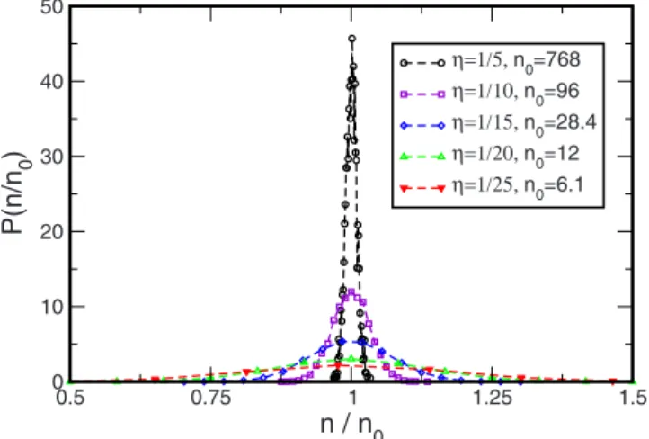
= l/L. Because of the fluidity in our system, the particle num-ber n in a small box of each realization fluctuates around the average value n0= N/N. As shown in Fig.2, for a small, n0is very small so that a small variation of n from boxes to boxes causes a large fluctuation on the particle ratio n/n0. The fluctuation of n is generally a result due to the topologi-cally disordered structures in our model. This is one of the differences between our model and the AM, in which the numbers of lattice points in every small boxes in the box-counting procedure are the same. Thus, the box-box-counting procedure for our model is nothing but a coarse graining of our system from particles with a unit size into the small boxes by a scaling factor l in length.
TABLE I. The system sizes of our simulations for the TLJ fluid atⴱ= 0.972 and Tⴱ= 0.836. N is the particle number and L =共N/ⴱ兲1/3is the length of simulation box. Both L andⴱare in the LJ units.
N 3000 6000 12000 24000 48000 96000
L 14.56 18.38 23.12 29.12 36.69 46.22
FIG. 1. 共Color兲 Geometric structure of the INM with 共a兲 = 1183.25 or 共b兲 −86.78 for the TLJ fluid of 96 000 particles in a box of L = 46.22. In each panel, particles with vibrational ampli-tudes 兩eis兩 larger than the average value N−1/2 are presented by
spheres with diameter of one and centered at particle position. The color of each sphere indicates the兩ejs兩 value of the particle. The total numbers of spheres presented in 共a兲 and 共b兲 are about 5700 and 7000, respectively.
Considering INM s of a configuration, we define a mea-surek
s共兲 as the sum of the squared vibrational amplitudes
of particles inside the kth small box with the expression as
k
s共兲 =
兺
j苸boxk兩ej
s兩2. 共2兲
The generalized inverse participation ratio Pq
s共兲 of this INM
is defined as a summation of the qth moment of k
s共兲 over
all small boxes. That is,
Pq s共兲 =
兺
k=1 N 关k s共兲兴q . 共3兲Due to the normalization condition in Eq. 共1兲, as q=1,
Pq
s共兲=1 for all INMs and all values of
. Then, we make a typical average on Pq
s共兲 over the INMs within a small
ei-genvalue window 关11,29,30兴. The typical average of Pq s共兲,
denoted as Pq共,兲, is defined as Pq共,兲 ⬅ exp ⬍ ln Pq
s共兲⬎
, 共4兲
where 具¯典 is an arithmetic average over the INMs with eigenvalues within a small interval of width⌬ and centered at.
Underlying the assumption of multifractality, which, in principle, has no relevant length scale, Pq共,兲 is assumed
to follow the power-law behavior
Pq共,兲 ⬀q. 共5兲
From this scaling relation,qis given as q= lim
→0
ln Pq共,兲
ln . 共6兲
The mass exponentqis a quantity characterizing the nature
of the INMs under the average:q= d共q−1兲 for the
delocal-ized INMs, where d is the space dimension andq= 0 for the
localized INMs. At the MEs, q= Dq共q−1兲, where Dq is the
so-called generalized fractal dimension. Generally, Dq
de-pends only on the universality class of the associated random
matrices so that Dq should be the same for the two MEs in
the INM spectrum. The value of Dq is less or larger than d
for positive or negative q, respectively.
In the multifractal analysis, the singularity spectrum f共␣兲 is a useful quantity, which can be obtained fromqthrough a
Legendre transformation, fq= f共␣q兲 =␣qq −q, 共7兲 with ␣q= dq dq, q = f
⬘
共␣兲. 共8兲The meaning of f共␣兲 for the INMs is given as the following: as long as the scaled linear size L
⬘
= 1/is large enough, the small boxes, which are specified with the coarse-grain squared vibrational amplitudes ks共兲 scaled as ␣
, form a fractal with a fractal dimension f共␣兲. That is, the number of such small boxes scales as L
⬘
f共␣兲. Alternatively, by consider-ing directly the particles in the fluid configuration of linear size L, f共␣兲 is the fractal dimension of the set of particles with兩ejs兩2⬃L−␣and, thus, the number of such particles scales as Lf共␣兲. In the typical average, the behavior of Pq共,兲 isgenerally dominated by a single representative INM关30兴. To make sure that the particle number scaling as Lf共␣兲 in the
representative INM is always larger than one, f共␣兲 under the typical average is always positive 关11兴 no matter what the value of L is.
According to the definitions given in Eqs.共7兲 and 共8兲 and
qin Eq.共6兲,␣qand fqcan be reformulated as the following
expressions: ␣q= lim →0 ln Tq共,兲 ln , 共9兲 fq= lim →0 ln Fq共,兲 ln , 共10兲 where ln Tq共,兲 =
冓
兺
k=1 N ␦k s共q,兲ln␦ k s共1,兲冔
, 共11兲 ln Fq共,兲 =冓
兺
k=1 N ␦k s共q,兲ln␦ k s共q,兲冔
, 共12兲 with ␦k s共q,兲⬅关 k s共兲兴q/ P qs共兲. With the sets of ␣
q and fq
calculated by Eqs. 共9兲 and 共10兲 for different values of the implicit parameter q, the function of f共␣兲 under the typical average is obtained such that the difficulties in numerical calculations via Eqs.共7兲 and 共8兲 are avoided.
IV. MULTIFRACTALITY OF INMs AT A ME In this section, we present the multifractal properties of the INMs at the MEs, including the generalized fractal di-mension and the singularity spectrum. We also show the probability density function and the spatial correlation func-tion of squared vibrafunc-tional amplitudes in the multifractal
0.5 0.75 1 1.25 1.5 n / n0 0 10 20 30 40 50 P(n /n 0 ) η=1/5, n0=768 η=1/10, n0=96 η=1/15, n0=28.4 η=1/20, n0=12 η=1/25, n0=6.1
FIG. 2. 共Color online兲 Distribution of particle number n in a small box in the box-counting method for the TLJ fluid of N = 96 000 particles. The symbols are the numerical results for several
INMs. The results presented in the following are averaged for the INMs with =−86.6⫾0.5 or those with = 1183.8⫾1.
A. Fractal dimension and singularity spectrum The thermodynamic limit in Eq.共6兲 is achieved by either
L→⬁ or l→0 but, practically, these two limits cannot be
obtained numerically for the discrete nature of our model due to particle size and the finite sizes of simulated systems. Instead of taking the limit, the value of q is interpreted as
the slope of ln Pq共,兲 versus ln as is very small.
Hence, this slope can be obtained numerically by a linear fit of the ln Pq共,兲 data within a finite interval of. Similarly,
the values of␣qand fqin Eqs.共9兲 and 共10兲 are obtained from
the slope of a linear fit for ln Tq共,兲 and ln Fq共,兲 versus
ln, respectively. By this approach, the three quantities ver-sus lncan be calculated in two different ways: the box-size scaling and the system-size scaling. In the box-size scaling, only one system with very large L is needed so that L is a constant and the variations of the three measured quantities with the box-size l are calculated. In the system-size scaling, all simulated systems with different L are partitioned into small boxes of the same size so that l is a constant and the variations of the measured quantities with L are evaluated.
In the box-size scaling, by averaging 5⫻103INM eigen-vectors of N = 96 000 at the ME in the negative branch and taking the scaled size L
⬘
= 1/as an integer varied from 2 to 10, we have calculated ln Pq共,兲, ln Tq共,兲, andln Fq共,兲 for q between −5 and 5. The numerical results of
integer q are presented in Fig.3, including the linear fit for the data of each q. Generally, for each q, the ln Pq共,兲,
ln Tq共,兲, and ln Fq共,兲 data have a linear behavior at
small ln. We have performed the same calculations at the positive-eigenvalue ME and the results are almost the same as those in Fig. 3.
In system-size scaling, we set l = 2.427 such that the simu-lated system of N = 3000 is exactly partitioned into 216 boxes, with L
⬘
= 6 and the average particle number n0= 13.9. For other larger simulated systems and with this l, L/l is not exactly an integer so that we partition each realization into small boxes of size l as many as possible, with some remains not enough to be a small box. In such a partition, the number of small boxes available is L˜3, where L˜ is the maximum integer which is smaller than or equal to L/l. Thus, for the six system sizes that we have simulated, the values of L˜ are 6, 7, 9, 12, 15, and 19; correspondingly, the definition ofin the system-size scaling changes as 1/L˜. For a partition with remains, only particles in those small boxes are involved in the calculations of ks共兲; however, by requiring that one corner of the partitioned box of size L˜ coincides with one of the simulation box, each realization may have eight different ways of partition, which enhances the number of sampling for statistical average. Calculated with the system-size scal-ing, the results of ln Pq共,兲, ln Tq共,兲, and ln Fq共,兲versus ln are close to those shown in Fig.3.
The mass exponentq and the generalized fractal
dimen-sion Dq=q/共q−1兲 at the two MEs are plotted in Fig.4 for
−5ⱕqⱕ5. The data obtained by the box-size scaling are accurate enough to indicate that q and Dq at the two MEs
are identical. At q = 0,q= −d and Dq= 0 as expected. For q
= 2, D2is the correlation dimension of the inverse participa-tion ratio P2 关28,30,31兴. The results of the box-size scaling give D2= 1.40⫾0.03, which is generally comparable with the D2 value of the AM estimated with the previously re-ported methods 关32–35兴. However, the value of D2 by the system-size scaling is 1.29⫾0.04, close to the value reported recently by the generalized multifractal analysis for the AM 关36兴. In principle, as q varies from −⬁ to ⬁, q is a
mono-tonically increase function of q, but the slope of the function, which is ␣q, decreases from the limiting value ␣+ to ␣−, which confines the range of the singularity spectrum f共␣兲 under the typical average 关11兴. Estimated by our data at 兩q兩 = 5 in Fig. 4共a兲, the value of ␣ by the box-size scaling is limited from 0.86 to 6.7; with almost the same upper limit, the range of␣by the system-size scaling is extended to 0.78. Presented in the insets of Figs. 5共a兲and5共b兲 are the val-ues of␣qand fqgenerated from the slope of the linear fit for
ln Tq共,兲 and ln Fq共,兲 with −5ⱕqⱕ5, respectively.
With the ␣q and fq data by the box-size scaling, the
singu-larity spectra f共␣兲 at the two MEs are plotted in Fig. 5共a兲. Within numerical errors, the singularity spectra at the two
0 20 40 60 80
ln
P
q(λ,
η)
q=-5 q=-4 q=-3 q=-2 q=-1 q=0 q=1 q=2 q=3 q=4 q=5 -12 -8 -4 0ln
T
q(λ,
η)
-2.5 -2 -1.5 -1 -0.5 lnη -6 -4 -2 0ln
F
q(λ,
η)
(a) (b) (c)FIG. 3. 共Color online兲 共a兲 ln Pq共,兲, 共b兲 ln Tq共,兲, and 共c兲 ln Fq共,兲 versus lnfor the INMs with=−86.6⫾0.5. The nu-merical data are obtained by the box-size scaling for N = 96 000, with the scaled size L⬘= 1/an integer from 2 to 10. The symbols are the numerical results, with the filled ones for negative q, the open ones for positive q, and the crosses for q = 0. The data errors are smaller than the symbol size. The linear fits for the data are indicated by either the black dashed lines for q⫽0 or the red solid line for q = 0.
MEs are generally identical and also agree with that of the AM at the critical disorder 关11兴. This agreement provides another confirmation for the locations of the two MEs in the INM spectrum. Indicated by our results, the maximum of
f共␣兲 occurs at␣0= 4.034⫾0.006 for the positive-eigenvalue ME and ␣0= 4.049⫾0.016 for the negative-eigenvalue ME; the two values of ␣0 generally agree with each other. Simi-larly, with the data of the system-size scaling, the singularity spectrum at the negative-value ME is presented in Fig.5共b兲, with␣0= 4.1⫾0.02 and the left end of the spectrum extended toward smaller␣as compared with the one obtained by the box-size scaling. The singularity spectrum generally agrees with that of the AM obtained by the system-size scaling关11兴, except for a small deviation in the right共large␣兲 end, which is attributed to the small average particle number and large fluctuations in the small boxes in our system-size-scaling calculations.
Around the maximum at␣0, where f共␣0兲=d, the singular-ity spectrum can be described by Wegner’s parabolic ap-proximation共PA兲 关37兴,
fPA共␣兲 = d −共␣−␣0兲 2
4共␣0− d兲, 共13兲 which is ensured to go through the maximum of f共␣兲 and to be tangential to the line f共␣兲=␣. As shown in Figs.5共a兲and 5共b兲, f共␣兲 deviates from the PA as␣is near either␣+or␣−, and the overall shape of f共␣兲 becomes asymmetric about the maximum of f共␣兲.
By substituting f共␣兲 in Eqs. 共7兲 and 共8兲 with fPA共␣兲,
q
and Dqunder the PA are given as q PA = −共␣0− d兲q2+␣0q − d, 共14兲 Dq PA = −共␣0− d兲q + d, 共15兲 where␣0is the only parameter. By setting␣0= 4.04,qPAand DqPA, as shown in Fig.4, are good only for small q.
Relative to the fully delocalized states, the anomalous di-mension of multifractals is defined as ⌬q⬅q− d共q−1兲.
Re-cently, based on the nonlinear model 关10,38,39兴, a sym-metric relation of the anomalous dimension is shown as -30 -20 -10 0
τ
q Positive eigenvalue Negative eigenvalue Parabolic approx. System-size scaling -4 -2 0 2 4q
0 2 4 6D
q(a)
(b)
FIG. 4. 共Color online兲 共a兲 Mass exponentqand共b兲 generalized fractal dimension Dqas a function of q. The black circles and red triangles are obtained by the box-size scaling for INMs with = 1183.8⫾1.0 and =−86.6⫾0.5, respectively. The green dia-monds are obtained by the system-size scaling for INMs with= −86.6⫾0.5. The data errors in 共a兲 and those around q=0 in 共b兲 are smaller than the symbol size. The dashed-dotted lines are the PA with␣0= 4.04. 0 2 4 6 8 α 0 1 2 3 f( α) Positive INMs Negative INMs Symmetric Parabolic approx. AM -4 -2 0 2 4 q 0 2 4 6 αq -4 -2 0 2 4 q 0 1 2 3 fq (a) 0 2 4 6 8 α 0 1 2 3 f( α) Negative INMs Symmetric Parabolic approx. AM -4 -2 0 2 4 q 0 2 4 6 αq -4 -2 0 2 4 q 0 1 2 3 fq (b)
FIG. 5. 共Color online兲 Singularity spectrum f共␣兲 of the INMs at a ME obtained by 共a兲 the box-size scaling and 共b兲 the system-size scaling. In共a兲, the INMs are calculated with =1183.8⫾1 共circles兲 and=−86.6⫾0.5 共squares兲 for N=96 000; in 共b兲, the INMs with =−86.6⫾0.5 共squares兲 are calculated for six system sizes from
N = 3000 to 96 000. In each panel, f共␣兲 is generated with the data of
␣q and fq shown in the insets for −5ⱕqⱕ5 with a step of ⌬q = 0.1. The green solid line is the corresponding spectrum trans-formed via the symmetric relation in Eq.共17兲. The red dashed line is that of the AM at the critical disorder 关11兴. The blue dashed-dotted lines in 共a兲 and 共b兲 are the PA with␣0= 4.04 and␣0= 4.10, respectively.
⌬q=⌬1−q. 共16兲 With the symmetric relation of ⌬q, it has been proved that
the f共␣兲 value for ␣⬍d and that for ␣⬎d are transformed with each other via the relation
f共2d −␣兲 = f共␣兲 + d −␣, 共17兲 where ␣ is only defined between 0 and 2d. The symmetric relation of⌬qhas been confirmed numerically for the
power-law random banded matrix model in one dimension关10兴, the symplectic Anderson model in two dimensions关40兴 and the orthogonal Anderson model in three dimensions关11,12兴 and evidenced experimentally by the ultrasound waves in two dimensions关18兴.
We also show in Figs. 5共a兲and5共b兲 the comparison be-tween the singularity spectrum of the INMs and the one gen-erated via the symmetric relation in Eq.共17兲. By the box-size scaling, f共␣兲 at a ME is generally satisfied with the symmet-ric relation within 2ⱕ␣ⱕ4, which is similar as the range for the AM. To examine the symmetric relation of ⌬q for the
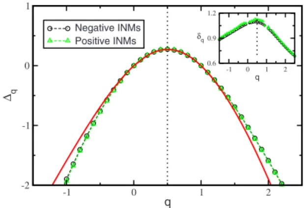
INMs at a ME, we plot in Fig.6the anomalous dimension⌬q
and compare ⌬q with⌬1−q, which is obtained by the mirror image of ⌬q with respect to q = 1/2. Our data of ⌬q at each
ME are satisfied with the symmetric relation for q between −0.5 and 1.5. Shown in the inset in Fig. 6 is the reduced anomalous dimension␦q=⌬q/q共1−q兲. Our result of ␦q
ver-sus q has a similar shape as the one measured by the multi-fractal ultrasounds on the surface of an elastic network关18兴. According to our results, we have shown that the INMs at the MEs behave in the same multifractal features as those of the lattice AM at the critical disorder. The agreement be-tween our results and those of the AM gives a numerical evidence for the universality of multifractals at a LDT. In the following, we investigate the vibrational amplitudes in the multifractal INMs and present only the results at the ME in the negative branch.
B. Probability density function
Another approach to characterize the multifractal INMs is the statistics of squared vibrational amplitudes in individual INM eigenvector. Averaged over the multifractal INMs of N particles in a system of size L, the PDF P˜L共兲 of the squared
vibrational amplitudes=兩ej
s兩2is defined such that P˜ L共兲⌬
is the ratio ⌬N/N, where ⌬N is the averaged number of particles with squared vibrational amplitudes lying between
and+⌬in an INM. By changing variable to the singu-larity strength ␣= −ln/ln L, the corresponding PDF PL共␣兲
is given as P˜L共兲d/d␣. Based on the physical meaning of f共␣兲, PL共␣兲 has a scaling of Lf共␣兲−d. Recently, it has been
proved analytically and confirmed with the numerical results of the AM in three dimensions 关13兴 that the proportionality of the scaling is the maximum value of the PDF at ␣0 be-cause of f共␣0兲=d. Thus, PL共␣兲 can be expressed as
PL共␣兲 = PL共␣0兲Lf共␣兲−d. 共18兲 Since the scale invariance of␣0 with system size, the posi-tion of the maximum PDF is expected to be independence of
L.
By using the PA of f共␣兲 in Eq. 共13兲, we obtain a Gaussian approximation 共GA兲 of PL共␣兲 as PL GA共␣兲 = P L共␣0兲exp
再
− 共␣−␣0兲2 4共␣0− d兲ln L冎
. 共19兲 Under the GA, the distribution width of PL共␣兲 decreaseswith 共ln L兲1/2, while the maximum PL共␣0兲 increases with 共ln L兲1/2 due to the normalization of the PDF. On the other hand, in terms of the symmetric relation of f共␣兲 in Eq. 共17兲,
PL共␣兲 for large enough L is expected to approach the one
generated via the symmetric transformation共ST兲,
PL
ST共␣兲 = L␣−dP
L共2d −␣兲, 共20兲
where 0ⱕ␣ⱕ2d. The equivalence of PL共␣兲 and PL
ST共␣兲 im-plies that the values of PL共␣ⱖd兲 and PL共dⱕ␣兲 are
corre-lated with each other. Therefore, the investigation of PL共␣兲
provides an insight into the property of f共␣兲.
Calculated with 7000 INM eigenvectors for each N from 3000 to 96 000, the variation of PL共␣兲 with system size is
shown in Fig.7. Located at␣= 4.1⫾0.04, the position of the
PL共␣兲 maximum is almost invariant with system size. Within
our numerical resolution, this maximum position is very close to the ␣0 value of f共␣兲 obtained by the system-size scaling in Fig. 5共b兲. Shown in the inset of Fig. 7, PL共␣0兲, with ␣0= 4.1, indeed scales as 共ln L兲1/2, which agrees with the prediction of the GA.
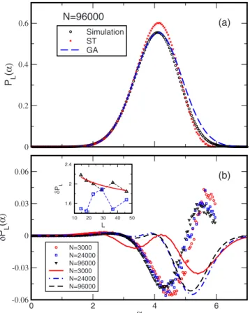
The comparisons of PL共␣兲 with PL
GA共␣兲 and P
L
ST共␣兲 are shown in Fig.8共a兲for N = 96 000. Our results indicate that a noticeable deviation of PL共␣兲 from the GA or the ST is found
in the large-␣region, which corresponds to small vibrational amplitudes. To quantify the deviation of PL共␣兲 from the GA
or the ST, we define the difference ␦PL O共␣兲= P
L共␣兲− PL O共␣兲,
where O is either GA or ST and the integrated difference
␦PL O
=兰0␣c兩␦P L O共␣兲兩d␣
, where␣c= 2d for O = ST and␣c= 7 for O = GA. The numerical results of ␦PL
O共␣兲 are presented in
Fig.8共b兲and the system-size dependences of␦PL
ST and␦PL GA -1 0 1 2 q -2 -1 0 1 ∆q Negative INMs Positive INMs -1 0 1 2 q 0.6 0.9 1.2 δq
FIG. 6. 共Color online兲 Anomalous dimension ⌬q and reduced anomalous dimension␦q共inset兲 versus q at a ME. Obtained by the box-size scaling, the circles and triangles, guiding the eye with the dashed line, are the⌬qdata of the INMs with =−86.6⫾0.5 and 1183.8⫾1, respectively. The data errors are smaller than the sym-bol size. The red solid line is the mirror image of the⌬qdata with respect to the line q = 1/2.
are in the inset of the figure. For the system sizes investi-gated so far, the integrated difference of the GA is generally smaller than that of the ST. However, the integrated differ-ence of the ST is found to decrease with increasing system
size, which is consistent with the result of the AM 关13兴. Fluctuating with the system size, the integrated difference of the GA does not decay with increasing system size, which implies the non-Gaussian nature of PL共␣兲 at even large
sys-tem sizes. Thus, our results suggest that, by increasing the system size of our model, the singularity spectrum f共␣兲 at a ME gets satisfied with the symmetric relation in Eq.共17兲 but not with the PA in Eq.共13兲.
C. Spatial correlation function
To characterize the spatial structures of the multifractal INMs, we define the spatial correlation function关41兴 for the
qth moment of the squared vibrational amplitudes of two
particles separated at a distance r in a system of size L as
Cq共r,L兲 =
冓
1 N兺
i=1 N兺
j⫽i N 兩ei s兩2q兩e j s兩2q␦共r − r ij兲冔
, 共21兲 where rijis the distance between particles i and j, thebrack-ets denote an ensemble average for the multifractal INMs, and r is assumed to be smaller than half of L. Since the distribution of squared vibrational amplitudes relies on the system size, Cq共r,L兲 not only is a function of the distance
between two particles but also depends on L. In terms of ⌬Nr, which is the number of particles within a spherical shell
between r and r +␦r about a central particle, the expression
of Cq共r,L兲 is written as Cq共r,L兲 =
冓
1 N⌬Nr兺
i=1 N兺
j=1 ⌬Nr 兩ei s兩2q兩e j s兩2q冔
, 共22兲where the second summation is subject to those particles within the shell.
Based on the multifractal nature, a scaling argument for the spatial correlation function of the critical states at the Anderson transition has been given关42,43兴. By applying the scaling argument for the squared vibrational amplitudes of the multifractal INMs, the scaling behavior of Cq共r,L兲 is
predicted as
Cq共r,L兲 ⬀ L−yq· r−zq, 共23兲
where yqand zq, the correlation exponents of the spatial
cor-relation function, are given as
yq= d +2q, 共24兲
zq= d + 2q−2q. 共25兲 By using the PA of q in Eq.共14兲, yq and zq in the PA are
expressed as
yqPA= 2␣0q − 4共␣0− d兲q2, 共26兲 zq
PA= 2共␣
0− d兲q2. 共27兲
To examine whether the correlation exponents of the mul-tifractal INMs follow the predictions of the scaling argu-ment, we calculate Cq共r,L兲 at the ME in the negative branch
for several system sizes. Presented in Fig. 9共a兲 are the
Cq共r,L兲 of N=48 000 with 0⬍q⬍2 for r less than L/2.
2 4 6 α 0 0.2 0.4 0.6 PL (α ) N=3000 N=6000 N=12000 N=24000 N=48000 N=96000 1.6 1.8 2 (lnL)1/2 0.48 0.52 0.56 PL (α0 )
FIG. 7. 共Color online兲 System-size dependence of PL共␣兲 for INMs with =−86.6⫾0.5. ␣=−ln兩esj兩2/ln L. The symbols denote
the numerical results with a resolution⌬␣=0.04. With ␣0= 4.10, the inset shows PL共␣0兲 versus 共ln L兲1/2and the fit of A + B共ln L兲1/2共red
solid line兲, with A=0.043 and B=0.261.
0 0.2 0.4 0.6 P L (α) Simulation ST GA 0 2 4 6 α -0.06 -0.03 0 0.03 0.06 δP L (α) N=3000 N=24000 N=96000 N=3000 N=24000 N=96000 10 20 30 40 50 L 1.6 2 2.4 δPL N=96000 (a) (b)
FIG. 8. 共Color online兲 共a兲 PL共␣兲 共circles兲, PL
GA共␣兲 共dashed line兲,
and PLST共␣兲 共crosses兲 for N=96 000. 共b兲 For N=3000, 24 000, and 96 000,␦PLGA共␣兲 are indicated by solid, dashed-dotted, and dashed
lines and ␦PLST共␣兲 are indicated by circles, squares, and triangles,
respectively. The inset shows the system-size dependences of␦PLGA
共squares兲 and␦PLST共triangles兲. The red solid line is the fit of AL−B
Evidenced by our results, Cq共r,L兲 indeed follows a
power-law decay with respect to r. We make a linear fit for the data of each q in Fig.9共a兲so that the data of zqare extracted. The
numerical results of zq are presented in Fig. 9共b兲, with the
error of zqestimated by a similar way given in Ref.关19兴. For
large q, the original data of Cq共r,L兲 suffer from strong
fluc-tuations, which cause large errors in zq. By substituting the
data ofqobtained by the box-size scaling or the system-size
scaling into Eq.共25兲, the predictions of the scaling argument are shown in Fig. 9共b兲 for comparison. Indicated by our re-sults, the scaling argument with q of the box-size scaling
agrees with the numerical data for q⬍1; however, withqof
the system-size scaling, the range in q for the agreement is extended up to 1.2. With␣0= 4.04 in Eq.共25兲, the PA of zqis
good for q⬍0.7, which is consistent with that the PA forq
is only good for small q.
Similarly, we calculate Cq共r,L兲 at a fixed r for several
system sizes of N varying from 3000 to 48 000. No qualita-tive difference is found in the system-size dependence of ln Cq共r,L兲, wherever r is set at 4.0, 4.5, 5, or 5.5, which are
distances around the fifth shell in the radial distribution func-tion but still smaller than half of L for N = 3000. With results
averaged for the four distances of r, ln Cq共r,L兲 versus ln L is
plotted in Fig. 10共a兲. The linearity of the data for each q in Fig. 10共a兲 indicates the power-law dependence of Cq共r,L兲
with respect to L and the slope of a linear fit gives the nu-merical data of yq, which are shown in Fig.10共b兲 with the
errors estimated in a similar way as those of zq. We have
examined the data of yq for ln Cq共r,L兲 evaluated at the four
distances of r; however, the variation of yqwith r is too small
to be noticeable. Again, with the q data obtained by the
box-size scaling, the prediction of the scaling argument for
yq agrees with the numerical results for q⬍1.2, which is a
little larger than that for zq. Similarly, by theq data of the
system-size scaling, the upper limit of the agreement extends to q = 1.4. However, the PA of yqin Eq.共26兲 is still only good
for q⬍0.7.
V. CONCLUSIONS
In this paper, we have investigated the multifractality of the INMs at the two MEs of a simple fluid, with the two MEs distinguishable by positive or negative eigenvalue. The loca-tions of the MEs were determined in a previous work by
1.5 2 2.5 3 ln r -40 -30 -20 -10 0 ln C q (r, L) 0 0.5 1 1.5 q 0 1 2 3 z q Numerical data Parabolic approx. Scaling theory (box-sizeτq)
Scaling theory (system-sizeτq)
(a)
(b)
FIG. 9. 共Color online兲 共a兲 Spatial dependence of Cq共r,L兲 in a log-log plot for N = 48 000. The symbols are the averaged results of INMs with =−86.6⫾0.5. The data from top to bottom are for q from 0.2 to 1.8 with a step of⌬q=0.2. The solid lines are a linear fit for each q. 共b兲 Correlation exponent zq versus q. The red filled squares are obtained by the linear-fit results in 共a兲. The dashed-dotted line is the PA. The black circles and green triangles are the predictions of the scaling theory withqobtained by the box-size scaling and the system-size scaling, respectively.
2.8 3.2 3.6 ln L -24 -16 -8 0 ln C q (r, L ) 0 0.5 1 1.5 q 0 2 4 6 y q Numerical data Parabolic approx. Scaling theory (box-sizeτq)
Scaling theory (system-sizeτq)
(a)
(b)
FIG. 10. 共Color online兲 共a兲 System-size dependence of Cq共r,L兲 in a log-log plot for an average over r at 4.0, 4.5, 5, and 5.5. The numerical data are for the INMs with=−86.6⫾0.5. From left to right, the system sizes N are from 3000 to 48 000; from top to bottom, the values of q are from 0.2 to 1.6 with a step of⌬q=0.2. The dashed lines are a linear fit for each q.共b兲 Correlation exponent
yqversus q. The lines and symbols are similar in meaning as those in Fig.9共b兲.
using the level-spacing statistics and the finite-size scaling 关19兴. We generalize the multifractal analysis for the INMs at a ME with the box-counting method, in which the simulated system is partitioned into small boxes of equal volumes. Be-cause of the fluidity of our model, the particle numbers in the divided small boxes fluctuate around an average value; this is a major difference between our model and the lattice AM. By means of the multifractal analysis under the typical average, we have calculated the generalized inverse participation ra-tios of the squared vibrational amplitudes in the INMs by the box-size and system-size scalings. The results of the box-size scaling indicate that the INMs at a ME are characterized in the multifractal nature and the multifractals at the two MEs yield the same results in generalized fractal dimensions and singularity spectrum. By both box-size and system-size scal-ings, the singularity spectrum of the multifractal INMs agrees well with that of the AM, which provides a numerical evidence for the universal multifractality at the localization-delocalization transition due to disorder.
We have examined the singularity spectrum of the INMs with the symmetric relation originally proposed for the non-linear model关10兴. Our results indicate that the symmetric relation is obeyed as our model is in a very large system size; a similar conclusion is also obtained with the AM关11,13兴. In principle, multifractals exhibit self-similarity for all length scales, indicating that no length scale is determined by the systems where the multifractals are produced. However, our model and the AM are discrete models with a fundamental length unit, which is the lattice constant in the AM or the particle size in our model. In a length scale comparable with the length unit of a discrete model, the basic assumption of multifractals breaks down for the model. We conjecture that this is the reason why the system sizes of our model and the AM should be extremely large in order that the singularity spectra of the two models are fulfilled with the proposed symmetric relation.
For the multifractal INMs, the PDF of the logarithm of squared vibrational amplitudes is calculated for several sys-tem sizes. Associated with the maximum of the singularity
spectrum, the location of the maximum PDF is invariant with the system size. For the system sizes we have investigated so far, the PDF of the multifractal INMs is deviated from a Gaussian distribution, which corresponds to the singularity spectrum under the PA, especially in the region for the small vibrational amplitudes. Indicated by our numerical results, the deviation does not decrease with increasing the system size.
The spatial characteristics of the multifractal INMs in a finite-size system are examined by the spatial correlation function for the qth moment of the squared vibrational am-plitudes of two particles. Being a function of the two-particle distance and the system size, the spatial correlation function is numerically evidenced to decay in a power law for each variable with a correlation exponent. By a scaling argument 关42,43兴, the two correlation exponents of the spatial correla-tion funccorrela-tion are related to the mass exponents of the multi-fractal INMs. With the mass exponents obtained by the box-size and system-box-size scalings, the predications of the scaling argument agree with the numerical results of the two corre-lation exponents at small q but are deviated at large q; the prediction by the system-size scaling produces a larger range of agreement in q than that of the box-size scaling. The de-viation at large q is possibly resulted from the different av-erages used in our calculations for the spatial correlation function and the mass exponents of the multifractal INMs, which are under the ensemble and typical averages, respec-tively. The deviation is expected to be improved as the mass exponents of the INMs are also calculated under the en-semble average, which produces better results in the singu-larity spectrum of the AM than the typical average does关12兴. The multifractal analysis for the INMs under the ensemble average will be one of our future works.
ACKNOWLEDGMENTS
We are indebted to Professor R. A. Römer for providing their data of the AM. T.-M.W. acknowledges financial sup-ports from the National Science Council of Taiwan, under Grant No. NSC 99-2112-M-009-003-MY2.
关1兴 P. W. Anderson,Phys. Rev. 109, 1492共1958兲.
关2兴 F. Evers and A. D. Mirlin,Rev. Mod. Phys. 80, 1355共2008兲. 关3兴 J. Billy, V. Josse, Z. Zuo, A. Bernard, B. Hambrecht, P. Lugan, D. Clement, L. Sanchez-Palencia, P. Bouyer, and A. Aspect, Nature共London兲 453, 891 共2008兲.
关4兴 G. Roati, C. D’Errico, L. Fallani, M. Fattori, C. Fort, M. Zac-canti, G. Modugno, M. Modugno, and M. Inguscio, Nature 共London兲 453, 895 共2008兲.
关5兴 H. Hu, A. Strybulevych, J. H. Page, S. E. Skipetrov, and B. van Tiggelen,Nat. Phys. 4, 945共2008兲.
关6兴 A. Lagendijk, B. van Tiggelen, and D. S. Wiersma,Phys. To-day 62共8兲, 24 共2009兲.
关7兴 A. Aspect and M. Inguscio,Phys. Today 62共8兲, 30 共2009兲. 关8兴 A. Richardella, P. Roushan, S. Mack, B. Zhou, D. A. Huse, D.
D. Awschalom, and A. Yazdani,Science 327, 665共2010兲. 关9兴 M. Schreiber and H. Grussbach, Phys. Rev. Lett. 67, 607
共1991兲.
关10兴 A. D. Mirlin, Y. V. Fyodorov, A. Mildenberger, and F. Evers, Phys. Rev. Lett. 97, 046803共2006兲.
关11兴 L. J. Vasquez, A. Rodriguez, and R. A. Römer,Phys. Rev. B
78, 195106共2008兲.
关12兴 A. Rodriguez, L. J. Vasquez, and R. A. Römer,Phys. Rev. B
78, 195107共2008兲.
关13兴 A. Rodriguez, L. J. Vasquez, and R. A. Römer,Phys. Rev. Lett.
102, 106406共2009兲.
关14兴 W. Garber, F. M. Tangerman, P. B. Allen, and J. L. Feldman, Philos. Mag. Lett. 81, 433共2001兲.
关15兴 J. J. Ludlam, S. N. Taraskin, and S. R. Elliott,Phys. Rev. B 67, 132203共2003兲.
关16兴 J. L. Feldman and N. Bernstein, Phys. Rev. B 70, 235214 共2004兲.
J. Phys.: Condens. Matter 17, L321共2005兲.
关18兴 S. Faez, A. Strybulevych, J. H. Page, A. Lagendijk, and B. A. van Tiggelen,Phys. Rev. Lett. 103, 155703共2009兲.
关19兴 B. J. Huang and T. M. Wu,Phys. Rev. E 79, 041105共2009兲. 关20兴 R. M. Stratt,Acc. Chem. Res. 28, 201共1995兲.
关21兴 M. L. Mehta, Random Matrices 共Academic Press, San Diego, 1991兲.
关22兴 A. Chhabra and R. V. Jensen, Phys. Rev. Lett. 62, 1327 共1989兲.
关23兴 T. M. Wu, W. J. Ma, and S. F. Tsay, Physica A 254, 257 共1998兲.
关24兴 T. M. Wu and R. F. Loring,J. Chem. Phys. 97, 8568共1992兲. 关25兴 M. Bollhöfer and Y. Notay,Comput. Phys. Commun. 177, 951
共2007兲.
关26兴 O. Schenk, M. Bollhöfer, and R. A. Römer,SIAM J. Sci. Com-put.共USA兲 28, 963 共2006兲.
关27兴 B. J. Huang and T. M. Wu, Comput. Phys. Commun. 182, 213 共2011兲, doi:10.1016/j.cpc.2010.07.015
关28兴 T. M. Wu and W. J. Ma,J. Chem. Phys. 110, 447共1999兲. 关29兴 T. Nakayama and K. Yakubo, Fractal Concepts in Condensed
Matter Physics共Springer-Verlag, Berlin, 2003兲.
关30兴 A. D. Mirlin and F. Evers,Phys. Rev. B 62, 7920共2000兲.
关31兴 D. A. Parshin and H. R. Schober, Phys. Rev. B 57, 10232 共1998兲.
关32兴 T. Terao,Phys. Rev. B 56, 975共1997兲.
关33兴 D. A. Parshin and H. R. Schober,Phys. Rev. Lett. 83, 4590 共1999兲.
关34兴 E. Cuevas, M. Ortuño, V. Gasparian, and A. Pérez-Garrido, Phys. Rev. Lett. 88, 016401共2001兲.
关35兴 A. Mildenberger, F. Evers, and A. D. Mirlin,Phys. Rev. B 66, 033109共2002兲.
关36兴 A. Rodriguez, L. J. Vasquez, K. Slevin, and R. A. Römer, Phys. Rev. Lett. 105, 046403共2010兲.
关37兴 F. Wegner,Nucl. Phys. B 316, 663共1989兲.
关38兴 A. D. Mirlin and Y. V. Fyodorov,J. Phys. I 4, 655共1994兲. 关39兴 D. V. Savin, H. J. Sommers, and Y. V. Fyodorov, JETP Lett.
82, 544共2005兲.
关40兴 A. Mildenberger and F. Evers, Phys. Rev. B 75, 041303 共2007兲.
关41兴 M. E. Cates and J. M. Deutsch,Phys. Rev. A 35, 4907共1987兲. 关42兴 K. Pracz, M. Janssen, and P. Freche,J. Phys.: Condens. Matter
8, 7147共1996兲.