Jwusheng Hu
Associate Professor.Shiang-Hwua Yu
Graduate Student.Shih-Chang Huang
Graduate Student.Department ot Control Engineering, National Cfiao-Tung University, Hsinctiu, Taiwan
Optimal MISO Repetitive Control
System Design Using Mixed
Time and Frequency
Domain Criteria
This paper presents an optimal repetitive controller design approach when both frequency and time domain criteria are considered. These criteria include limited control force, convergence rate, and robustness. In particular, the design formulation is based on MISO (multiple-input-single-output) plants which aim at solving nodal point problems encountered inflexible dynamic systems. Nodal points represent physi-cal constraints for feedback control, especially when their frequencies are within the control bandwidth. If multiple control paths with distinct nodal frequencies are available, the proposed method is able to design controllers to compensate the effect and reach certain design objectives. The ellipsoid algorithm is used to calculate controllers' parameters. Experiments were conducted to demonstrate the proposed method.
1 Introduction
Repetitive control algorithms using internal model principle (Francis and Wonham, 1975) have been studied by many re-searchers (Tomizuka et al., 1988; Hara et al., 1988). Applica-tions such as noncircular cutting (Tsao and Tomizuka, 1988), disk drive tracking (Chew and Tomizuka, 1990), repeated mo-tion of robot manipulators (Sadegh et al., 1990), material test-ing (Shaw and Srinivasan, 1993), and active harmonic noise cancellation (Hu, 1995a) have been reported in literature. When a plant has unstable zeros near the unit circle, it has been shown that conventional design approaches such as adding zero-phase filters (Hu et al., 1995b) may not give satisfactory result. Fur-ther, several design issues need to be addressed when dealing with distributed systems or when the fundamental period of the disturbance is high:
1 Robustness—especially around nodal points (those zeros close to the unit circle) where accurate identification is difficult due to a low SIN ratio.
2 Convergent speed—closed-loop poles inevitably ap-proaching the unit circle due to a high fundamental period.
3 Limited control force—system may become unstable when the control force is saturated.
All these issues clearly indicate that an optimization scheme is necessary to select proper control parameters.
Nodal points in distributed parameter systems are actually transmission zeros of the plant. Attempting to cancel distur-bances whose frequency contents are in the neighborhood of these zeros results in a very large control force. An obvious way to avoid this problem is to change transmission zeros' locations by properly placing actuators or sensors. Alternatively, for MIMO systems, it is possible to arrange actuators such that transmission zeros of all input paths are distinct. In this case, each controller should "give u p " its control effort around its transmission zeros. These considerations represent various con-straints when performing optimization.
This paper proposes an optimal design approach to an MISO (multiple-input-single-output) repetitive control problem. It is Contributed by the Dyitamic Systems and Control Division for publication in
the JOURNAL OF DYNAMIC SYSTEMS, MEASUREMENT, ANI5 CONTROL. Manuscript
received by the DSCD July 28, 1995, Associate Technical Editor: Tau-Chin Tsao.
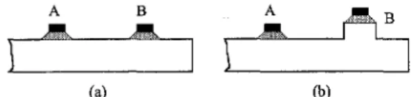
motivated from an experimental observation of active noise control in ducts. When mounting control speakers on the side of a duct, there is a great chance that the generated sound wave of some particular frequencies will be self-destructed (transmis-sion zeros). These frequencies are closely related to the dimen-sions and boundary conditions of the duct (Hu, 1995). From the explanation in preceding paragraphs, the control system's performance is limited when some of these frequencies fall into the bandwidth of design. Intuitively, multiple speakers can be arranged such that each speaker's transmission zeros are differ-ent to others. For example, as shown in Fig. 1, speaker B will have different transmission zeros from A when an additional segment of duct is added.
The organization of this paper is the following; Section 2 describes the problem formulation; Section 3 presents the solu-tion procedures and Secsolu-tion 4 explains the experiments con-ducted to verify the design methods.
2 M I S O Repetitive Control System Design
The block diagram of an m-input-1-output repetitive control system is depicted in Fig. 2. In Fig. 2, P, is the dynamic of each control path, C, is the compensator for each path and A^ represents multiplicative uncertainty, / = \,2, . . . , m. d repre-sents a periodic disturbance and M is the repetitive signal gener-ator. It is assumed that both /"j's and A,'s are stable dynamics. Let Pi = Pi{\ + A , ) , / = 1, 2, . . . , OT, and the multiplicative uncertainty A, satisfy
| A , ( w ) | = P, - Pi Pi
a{io) Va;[0, TT].
and ;• = 1, 2 . . . , m where a(a;) is a conservative estimate of the uncertainty bound. 0,
2.1 Stability and Robustness Analysis. When A
the internal stability of Fig. 2 requires that
-"c
1 - z~"(l - PC) G RH„ (2.1)
A sufficient condition to guarantee stability by using the small gain theorem is (P is assumed stable)
(a) (b)
Fig. 1 (a) Same transmission zeros of A and B; (b) different transmission zeros ( C I ) (C2) ''C e RH„ - P C L < 1 (2.2) (2.3) Note that from Eq. (2,2), C is allowed to be non-causal. When A =jS: 0, other than these two conditions, an additional condition should be added.
(C3) z-^PC
1 - z - ' ' ( l - P C ) < 1
sup |Ai(w) Vw (2.4)
At repetitive frequencies, i.e., uj = Ik'nlN, fe = 0, 1, . . . , NI2, we have.
" P C
1 - ^ - ' ' ( l - P C ) = 1
From Eq. (2.4), the maximum allowable perturbation is also 1 which limits the robust performance. Therefore, a filter is added to sacrifice disturbance rejection ability or tracking accuracy in order to gain robustness, i.e., the repetitive signal generator is changed into
M = qz 1 - qz-''
where q is the selected filter (Tsao and Tomizuka, 1988). By adding this filter, the stability and robustness conditions ( C I ) to (C3) are modified as (C4) z-'^qC e RHoo (C5) 111 - PC||„ < 1 (C6) z-^qPC
1 - z A ( l - P C )
< 1 sup | A j ( w ) | (2.5) (2.6) Vw (2.7)A more relaxed stability condition of (C5) should be ||^(1 -PC||„ < 1 since | ? ( w ) | < 1. However, implementing (C5) in design will result in more robustness since when | ^ ( a ; ) | is small.
z-yc
1 - z-^qil - P C ) « I^PCI <2\q\. (2.8)
Thus, if q is selected as an FIR low-pass filter, more high-frequency model uncertainty can be tolerated. In fact, an ideal selection of q should be
q(oj) = I, w e n , and | ^ ( w ) | = 0 , w ^ 51. (2.9)
where Q is the desired frequency range of disturbance rejection or tracking.
2.2 Performance Analysis. Two different performance requirements are investigated in this section. The first one is the speed of convergence. Assuming the z-transform of a periodic disturbance d is (denoted as d)
d =
1 F=fo+Az-' + ... +fN-iZ- (2.10)
The error of the repetitive control system, with the filter q added, is derived as (Fig. 2 ) ,
(1 - qz-") F__ [1 - z - " ? ( l - P C ) ] (1 - z - " ) (2.11) When qie'^''^"') i=s 1 and N is large, it can be seen that the convergence of the error at repetitive frequencies depends on the closed-loop poles. To reduce the design complexity, the plant P is assumed to be stable and its poles are canceled di-rectly. Further, if q and PC are FIR filters (by restricting the structure of C (see Eq. (3.4) later)), the closed-loop character-istic equation is
z"-""" + z % ( z ~ ' ) [ l - P ( z - ' ) C ( z ~ ' ) ] = 0 (2.12)
where Np is the number of poles of ^ ( z " ' ) P ( z ~ ' ) C ( z ^ ' ) at origin. Notice that ^ ( z ~ ' ) P ( z " ' ) C ( z ~ ' ) may be noncausal. Let the characteristic roots be re-'", 0 < r < 1, by maximum modu-lus theorem, we have
r"^^ = \z^q{z'){\ P ( z ' ) C ( z ' ) ] L . „
< Max | z ^ ? ( z ' ) [ l P ( z ^ ' ) C ( z ' ) ] | , . , . -^ | | 1 - P ( z - ' ) C ( z - ' ) | | c „ (2.13) since z''p^(z^')P(z~')C(z~') is analytic inside the unit circle and q is low pass (Eq. (2.9)). As a resuh, a proper constraint to limit the close-loop spectral radius is then,
111 - PCIU < <5
If the performance range (i.e., f2 in Eq. (2.9)) is considered, a more detailed constraint can be constructed as
(C7) s u p | l - P C | sup 11 PCI
< 8 and
< 1 (2.14)
Second, to avoid control force saturation, it is necessary to constrain controllers' output levels according to their physical limits. An obvious choice is the A-norm minimization (or 1, minimization) (Vidyasagar, 1986; Dahleh and Pearson, 1988), i.e., from Fig. 2,
lir„,JUMlU, i = 1,2, . . . , m ,
where T„^ = -Z-^Q
1 - z - " ( l - PC) ' this leads to the following condition (with the filter q added):
(C8) ||r„,JU^A, 7-^ = 1 1 ]f' p^,
1 - z q{\ - PC)
for i=\,l,...,m. (2.15) where /0,||(i|U is less than the saturation limit of the actuator ;.
3 Mixed Time and Frequency Domain Optimization
As explained by the design conditions ( C 4 - C 8 ) , controllers can be calculated by optimizing various time and frequency domain criteria (Boyd et al., 1988; Helton and Sideris, 1988; Khargonekar and Rotea, 1991; Sznaier, 1994). For example, if
Fig. 2 Biocl( diagram of an MISO repetitive control system (P = [P^ P2
... P„], C = [C, C2 . . . C„y, A = dlag (A,, Aa A„) and u = [u, ui...u„y)
we want to minimize the control forces under the constraint of a designated convergence speed, we could select:
min max||r„,JL, (3.1) subject to 111 - PC|U < 6, (5 < 1 (3.2) Similar problems of this type are in the area of convex optimiza-tion. Two commonly-used algorithms to solve these problems are the decent and nondecent methods. Non-decent methods such as the ellipsoid algorithm (Boyd and Barratt, 1991) are particu-larly suitable for nondifferentiable norms hke fto or Ij. To imple-ment the ellipsoid algorithm, it is necessary to calculate general-ized gradients of cost and constraint functions at each iteration (Boyd and Barratt, 1991; Clarke, 1975; Polak, 1987). In this paper, we present the solutions in finite dimensional space (i.e., suboptimal solutions). To realize the numerical calculation, it is necessary to formulate the cost function and constraints in vector notations as explained in the following sections.
3.1 Vector Space Representations of the Control Sys-tem. The plant is represented as the following,
P = [P, P2 . . . P „ ] , P,- = z - " . B , ( z - ' ) G , ( z " ' ) ,
i = 1, . . . , / n (3.3) where rii is the delay steps of Pi, Gi is minimum phase, and B, contains all zeros outside the circle centered at origin with radius ,3 < 1. The selection of f3 is to avoid stable pole-zero cancellations close to the unit circle since those zeros may not be accurately identified due to poor S/N ratios (nodal points as explained before). Let n be the maximum order of Bi's, i = 1
~ m, and
Biiz"') = b'o + bL,z-' + ... + bL„z'"
where some of the coefficients may be zero if the B,'s order is less than n.
The structure of C is selected as
C = [C, C2 . . . C„], C,. = z"'Di{z, z-')GT\z''),
i=\,...,m (3.4)
where
A ( z , z"') = d\z' + rfi-iz'"' + . . .
+ d'-MZ-'-*-' + dL,z-' (3.5)
By using Eq. (3.5), we shall perform optimization in finite dimensional space. Further, the filter q is assumed to be
q{z, z"') = qrZ'' + qr-iz'"'^ + . . . + ^0 + • • • + q-rZ'". (3.6)
The following formulae will be used in derivations later. (a) D , ( z , z - ' ) = [z' z'-' ...z-']d„
where d, = [rfi d',-i ... d'-tV (3.7) (b) z-'^^"9(z, z-')Di(z, z - ' ) = [1 Z-' . . . z - ' " " ^ ' ] Q 4 , O e R ( n + 2 ( + l ) X ( 2 ; + l ) d= \^f | e R ™ ( 2 ( + l ) X l ^ ^ , ^ d\ d'l-i d'-, (' = 1 m , e = 0,xl 1 0(„+()xl (3.9) (d) 9 ( 1 - I s , A ) _ r^'+r _ l + r - l -(/+n+r) ] Q ( e - Bd), where Q =1 O ^Ir I g Jj(n+2(+2r+l)X(/!+2/+l) / g iQ-.
3.2 Frequency Domain Design. The related functions in
frequency domain are (C6) and (C7). Since the filter q can be shaped to gain robustness (Eq. (2.8) and (2.9)), we focus the discussion on (C7). Using the vector notations in Eqs. ( 3 . 7 )
-(3.10), we have
1 - S S,A
= Re {(©'^e - 0 ^ d ) * ( 0 ' ^ e - © ' B d ) ) = (e - Bd)'^Re{©(e-^'^)0''(e^")}(e - Bd) (3.11) where&ien = le''"e y;u).j((-l)i. -j(;+n)ijl7-Re {Qie-n&'Xe'")]
Re [e"" e Jiu ,J(l-l)iu
1 cos ui COS 2u) cos (2/ + n)u y knowing that
111
-cos u 1 cos u cos (2/ + n -PCII^ = 111 l)w COS 2oj cos uj 1 m - I BiD,\\l cos(2/ + n)LO cos UJ 1 where Q = * ' - ^ . O O ^"-q-r, i ( 2 ; + 2 r + l ) X ( 2 / + l ) (3.8) = sup|l - I i B , A | ? = . - , (3.12) the generalized gradient g for ||1 - PC||i is derived by the maximum rule (Boyd and Barratt, 1991) asg = - 2 B ' ' R e {0(e-^'*'o)0'-(e>o)}(e - Bd) (3.13)
where (c) 1 - £ BiDt = [z' z'"' . . . z~<'''"*](e - Bd), where
B = [ B , B2 . . . B „ ] G R(«+2'+l)x»,(2/+l)
Wo e {w G R\ 111 - PC||„ = |1 - PCU=,/"}. Equation (3.13) can be modified to include a weighting func-tion. Other than the infinity norm, the H2 norm is also a good
index for minimizing the magnitude of (1 - PC) (under certain
smooth conditions), i.e.,
r, =
VA
111 - PCII^ = (e - Bd)^(e - Bd) (3.14) The corresponding generalized gradient can be easily derived
g ( d ) = - 2 B ^ ( e - Bd) (3.15)
1 -z^'qil - lD,B,)
1=1
The optimization is now focused on WTIWA instead of ||r„,rf||^. Suppose {>',(^)} represent the impulse response of I) and
{x(k)] an impulse input sequence, we have
There is a great flexibility of using the idea of H2 norm in selecting the performance range (i.e., Q in Eq. (2.9)). For example, if we wish to improve convergence at cj £ [wi, W2] and gain robustness at w G [ws, W4], we could use the following formula y,ik) = ie --BdVQ' y,(k- N + I + r) y,{k - N + I + r - 1) yiik - N + I + r - n) where min{||W,(l - P C ) | | 2 + ||W2PC||2]
_ 1 Vol G [wi uj^]
Wi{uj) = \ and 0 otherwise (3.16) + d f Q ' x{k) x{k- 1) x{k - 11 - 2r) fc = 0, 1, 2, (3.21) W2(LO) =
1 Vo) G [U>3 iU^] 0 otherwise
As a result, the representation of Eq. (3.16) in vector space are mm
where
| l - l B , A l ' r f w + | l B i A | ' r f w [ (3.17
|1 - J^B,D,\'-duj+ l l B . A l ' r f c
(e - Bd)'Wi(e - Bd) + d'B'WjBd (3.18)
To minimize the computational load, / (length of the filter D,) and r (length of the filter q) are restricted to satisfy {I + r) <
N/3. Under this restriction, the first N + I + r + \ terms of
the impulse response, i.e., {3',(*:)}t'=o"^', are
MO) yt{l) . . . >',(2/ + 2 r ) ] ^ = Q d , - (3.22a)
[>',(2/ + 2 r + 1 ) y,i2l + 2r + 2) ... y^iN - I - r - l)V
— 0(Ai_3(_3r_i)xl (3.22b)
[yi(N-l-r) y,{N-l-r+\) ... y^N + I + r)Y = Y,Q(e - Bd) (3.22c) where n{uj) = sin uj sin loj sm w w sin ui sin 2w 2 sin oj
sin {21 + n)ijj sin (2/ + n — \)tjj
21 + n 21 + n- I sin {21 + n)u) 21 + n sin u> and Wi = Q.{LJ2) - n ( w , ) , W2 = rJ(W4) - f^(W3) The generalized gradient is therefore derived as,
g = - 2 8 ^ ^ 1 ( 6 - Bd) + 2 B ^ 2 B d (3.19) 3.3 Time Domain Design. In minimizing the A-norm
in-dicated in (C8) (Eq. (2.15)), we limit the li norm of the impulse response from disturbance input to control forces. Since a closed-form representation of IT^.d lU is impossible due to infi-nite terms in the impulse response, a simplified approach is used. Observe first that (see Eqs. (2.15), (3.5), and (3.6))
Y = y.d) 0 y,(0) 0 . . . 0\ . . . 0
r.„
where - ( r + O qD,G-z""?(l - I s , A ) 1=1yy,(2/ + 2r) y,(2Z + r- \) ... yi{Q) 0 . . . 0/
g | » ( 2 ; + 2 / ' + l ) X ( n + 2 ( + 2 r + l )
Now the target function ||r,||^ is approximated as N+l+r
r / ( d ) I U « I | y , ( * , d ) | (3.23) According to Sznaier (1994), the error of this approximation
can be estimated. Assume that r, ( z " ' ) is analytic for every |z| a 5, 0 < 5 < 1, we have
^ l|r,IUIGr'IU (3.20)
yi{k)\ = 1 ^ ^ui=,r,(z"')z'"Vz
||r,^IU.,6* (3.24) whereDuct'.s length; 0.5m Cross Section; 0,15m x 0,15m Ciit-ol'f Frequonuy; 115.^ Hz
Fig. 3 Experimental setup
mi,s =
sup|r,.(z^')|.=&^-Therefore, the approximation error can be derived as
k=N+l+r + t
lir.ii ,A<''+'+'-+i)
|y,(fe)| ^ll^-ll-.f (3.25)
1 — 0From Eq. (3.25), the error is small if N + I + r + 1 is large or 6 is small. Note that S is the spectral radius of the closed loop system. Using the sum rule (Boyd and Barratt, 1991), the generalized gradient for the approximated function (Eq. (3.23)) is,
2 / + 2 r + l
8i(d) = X sign (yi(k- l ) ) v ,
k=l
+ sign (y,(k + N - I - r - 1))
X [-BWy/k + XtQ(e - Bd)} (3.26) where
0(i-l)(2/+l)x(2/+2r+l) Vj. is the k-th column vector of Q'^
_0(m-/)(2(+l)X(2;+2r + l) . Wj is the k-th column vector of Y f (see Eq. (3.22c)) and
X* = [Vi Vt_ O: m (2/+1) X (n+2;+2<' + 1 - * ) J
4 Design Examples and Experiments
Using the results derived in Sections 2 and 3, a design strategy was implemented. Experiments were conducted on a rectangular duct made of plastic glass. A DSP system based on TMS320c31 was installed to calculate the control signals (Fig. 3 ) . The sam-pling rate was chosen as 4 kHz. The calibration value of the error microphone is 49 mV/Pascal. A noise speaker was in-stalled to simulate a noise source. Two control speakers were
0 500 1000 1500
Frequency (Hz)
Fig. 4 Frequency response of plant Pi(z'') and Pi(z~'')
2000
Table 1 Unstable zeros of both plants (stability margin = 0.98; *\ transmission zeros within the bandwidth)
Bi d"') Bi (z-') zeros 1 2 3* 4 5 -3.4127 1.0302 0.7336 ± 0.6598/' -0.4907 ± 0.8598/--0.1766 ± 0.975V 1 2 3* 4* 5 -2.0429 1.0341 0.9366 ± 0.3031; 0.4463 ± 0.8816J -0.3009 ± 0.9545;
mounted on the side of the duct. One of them included an additional duct segment to prevent identical nodal points for both control paths. It should be emphasized that the setup is not a 1-D problem because the length (0.5m) is too short to ignore evanescent modes (Morse and Ingard, 1968; Doak, 1973). Hence, the behavior of nodal points is a 3-D phenome-non in this case.
The plant Pi (speaker 1) and P2 (speaker 2) are identified using time-domain least square algorithms with frequency weighting (weighted band = 0 ~ 1 KHz). Numerical calcula-tions were carried out by the identification toolbox of MAT-LAB. Their frequency response are depicted in Fig. 4, The total number of parameters for P^ and P2 are 56 (4 delay steps; 30 poles; 26 zeros) and 52 (4 delay steps; 28 poles; 24 zeros), respectively. Other than 0 Hz, plant P, has a transmission zero around 470 Hz and P2 around 200 and 700 Hz. They are differ-ent because a small passage to the duct is added to speaker 2 (Fig. 3). The zero at 0 Hz are common to both plants. This is the zero caused by AC-coupling of the power and microphone amplifier and is impossible to remove. As shown later, special treatment has to be done to prevent DC drift in control signals. To avoid stable pole-zero cancellation near the unit circle, the stability margin is selected to be 0.98. As a result, the non-minimum phase parts of both plants are listed in Table 1 (see Eq. (3.3)).
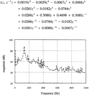
Figure 5 shows the spectrum of the periodic noise tested. Its fundamental period is 245 samples (A^ = 245; fundamental frequency is 16.32 Hz under 4 kHz sampUng). From Fig. 5, it can be seen that the noise signal is mostly within 500 Hz. Therefore, a zero-phase low-pass filter with cut-off frequency 666.7 Hz is selected for the filter q, i.e.,
q{z, z"') = 0.0019Z'' - 0.0029z'* - 0.0067z' + O.OOSSz" + 0.0261z= - 0.0182Z'' - 0.0784z' + 0.0266z' + 0.3080Z + 0.4698 + 0.3080z"' + 0.0266Z-' - 0.0784z~^ - 0.0182z-'' + 0.0261Z-' 4- O.OOSSz^' - 0.0067z~' 80 40
r'''iMi
0 200 400 600 800 1000 Frequency (Hz)Fig. 5 Spectrum of the liarmonic noise (recorded from a four cylinder engine)
0 200 400 600 800 1000 Frequency (Hz)
Fig. 6 Frequency responses of B,'s (Eq. (3.3)) with added filters to give up control around nodal points
0.1 0,08 0.06 0.04 0.02 0 -0.02 -0.04 -0.06 -0.08
i |
, , . . . : . . J l . , . . . j , . . i . . ^ . : . t . . . , . . , : . . A . . i . : . . . ; ^ . . A . '• • V- \ : i - r r i i ' 1-r r t - • i V i v - • -M IT . . . r . i ...;..,.!J...u:.l...I...^'...,...•..>.,... ..v'..i.i..i.)... ...'/...•....:.f,,.li...r.•,..i'...Ij...v...t(...-V.i.V..«...;...v.,.i(... 0.02 0.04 0.06 time (sec) 0.1Fig. 8 Steady-state noise signal before and after cancellation
- 0.0029Z-* + 0.0019Z-' (4.1) Within this bandwidth, the transmission zero of plant P^ is close to the 29th harmonic frequency of the noise (473.47 Hz) and Pj to the twelfth (195.91 Hz) and 43rd (702.04 Hz) harmonic frequency. Like the dc component, controller for each plant has to give up cancellation at the corresponding frequencies.
Base on observations from plant identification, several design principles are listed as the following:
• Give up cancellation of noise around dc and nodal points; • Enhance high-frequency robustness property;
• Improve convergence speed and noise rejection ability within the bandwidth;
• Keep control forces as small as possible.
To give up cancellation of noise around dc and nodal points, the corresponding internal models are added to the numerator of the signal generator M knowing that the controllers' internal states will not diverge if the error signal pass through the numer-ator first. In design stage, this means adding a series of filters to the plants. As a result, the frequency responses of Sj's (Eq. (3.3)) are plotted in Fig. 6. Further, two frequency segments of the open loop gain (| PC | or 11 - X ^ . A-1) are selected to satisfy:
• Unit magnitude and zero phase at frequency range 6.7 ~ 600 Hz;
• Magnitude as small as possible at frequency range 720 ~ 2000 Hz.
which represent disturbance rejection and robustness require-ments, respectively.
The optimization problem is then proposed as
min {(e - B d ) ^ i ( e - Bd) + d'B'WaBd) (4.2) Subject to
sup
lly,(d)||il|Gr
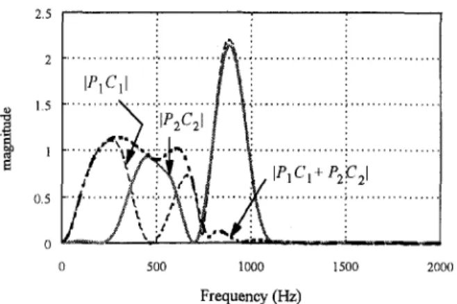
s u p ( e - B d ) ^ R e {0(e-^^'*')0^(e-'")}(e - Bd) I < 1 (4.3) where W, = n(0.37r) - n(7r/300), Wj = n(7r) - Q(0.367r) and c is the maximum saturation level for the actuators. The length of D] and D2 were chosen to be 37 (see Eqs. (3.4) and (3.7)) and the problem was solved by using the ellipsoid algorithm (Boyd and Barratt, 1991). Detailed iterative proce-dure is shown in the appendix but lengthy numerical results are not shown here (see Yu, 1995). The shaped loop gains are depicted in Fig. 7. From Fig. 7, the design objective was satis-fied since each control path gave up control effort around corre-sponding nodal points and the overall loop gain was shaped to have good convergence property within the bandwidth.
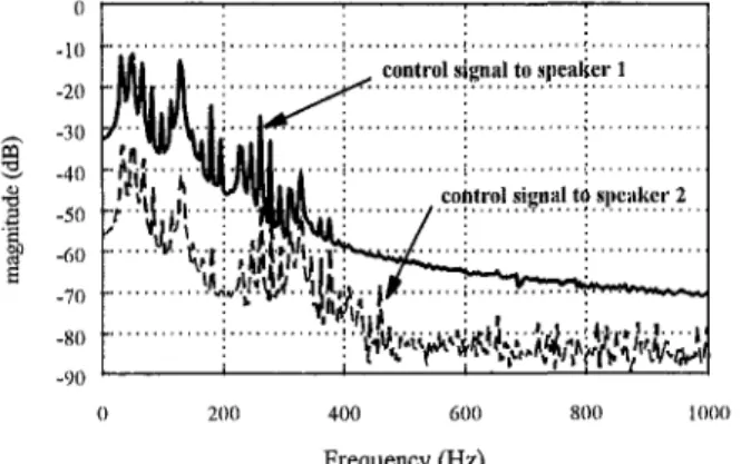
Figure 8 shows the error versus noise signal measured at the feedback microphone while Fig. 9 shows their spectrum. Figure 9 indicates that the controller effectively cancel noise under the bandwidth limited by the filter q (Eq. (4.1)). Within 1 kHz, an average of 12.7 dB noise reduction was achieved. To see if each control path gave up its effort around nodal points, the spectrum of steady-state speaker input signals are plotted in
0 500 1000 1500 2000
Frequency (Hz)
Fig. 7 Open-loop gains for individual and overall control paths
noise befor^ cancellation; VAJ ^Vi , ;^V- r ,; : noisc:aftcr cancelliiticin I'l V - . ' ' ! • , , i : ^ • ( ! -.1 • • • •
0 200 400 600 800
Frequency (Hz)
Fig. 9 Spectrum of noise before and after cancellation
0 -10 •• -20 •• ^ - 3 0 3 -40 3 -50 I -60 E -70 -80 -90
control signal to .speaker 1
m
V ' : 'Will' II' :•4^'
0 200 400 600 800 1000
Frequency (Hz)
Fig. 10 Spectrum of the steady-state control signals
Fig. 10. Around 200 and 700 Hz, speaker 2 generated no control signals. Speaker 1 essentially gave up control at high frequency range including its nodal point (470 Hz).
5 Conclusion
In this paper, we present a new approach to design repetitive controllers. Comprehensive design goals involving robustness and performance are formulated as frequency-response or im-pulse-response constraints on some system functions. In order to solve this mixed frequency-domain and time-domain prob-lem, the controller's structure is restricted to be finite dimen-sional. An interesting application of repetitive control is active harmonic noise cancellation (see Hu et al., 1995b). Because of the geometric constraint in wave propagation, one-loudspeaker ANC (Active Noise Control) system has some performance limits due to nodal points. Therefore, we designed a MISO repetitive ANC system and the proposed optimization tech-niques were applied. Experiments was conducted to demon-strate the effectiveness of this design approach.
Hu, Jwu-Sheng, Yu, Shiang-Hwua and Hsieh, Cheng-Shiang, 1995b, "On the Design of Digital Repetitive Controllers Using I2 and H» Optimal Criteria with Application to active harmonic noise cancellation in ducts," in Proc. 1995 ACC. Khargonekar, P. P., and Rotea, M. A., 1991, "Mixed H j / H . Control: A Convex Optimization Approach," Automatica, Vol. 36, No. 7, pp. 824-837.
Morse, P. M., and Ingard, K. U., 1968, Theoretical Acoustics, Princeton Univer-sity Press.
Polak, E., 1987, "On the mathematical foundations of non-differentiable opti-mization in engineering design," Society for Industrial and Applied Math. Review, Vol. 29, No. 1, pp. 21-89.
Polak, E. and Salcudean, S. E., 1988, "On the Design of Linear Multivariable Feedback Systems Via Constrained Non-Differentiable Optimization in H«," IEEE Transaction on Automatic Control, Vol. 34, No. 3, pp. 268-276.
Sadegh, N., Horowitz, R., Kao, W. W., and Tomizuka, M., 1990, " A Unified Approach to Design of Adaptive And Repetitive Controllers for Robot Manipula-tors," Trans, of the ASME. Vol. 112, pp. 618-629.
Shaw, F. R., and Srinivasan, K., 1993, "Discrete-Time Repetitive Control Sys-tems Design Using The Regeneration Spectrum," ASME JOURNAL OF DYNAMIC
SYSTEMS, MEASUREMENT, AND CONTROL, Vol. 115, pp. 228-237.
Sideris, A. and Rotstein, 1993, "Single Input-Single Output H« Control with Time Domain Constraints," Automatica, Vol. 29, pp. 969-984.
Sznaier, Mario, 1994, "Mixed li/H„ Controllers for SISO Discrete Time Sys-tems," Systems & Control Letters, Vol. 23, pp. 179-186.
Tomizuka, M., Tsao, T. C , and Chew, K. K., 1988, "Analysis and Synthesis of Discrete-Time Repetitive Controllers," American Control Conference, Atlanta. Tsao, T. C , and Tomizuka, M., 1988, "Adaptive and Repetitive Digital Control Algorithms for Non-circular Machining," in Proceedings 1988 American Control Conference, Atlanta, pp. 115-120.
Vidyasagar, M., 1986, "Optimal Rejection of Persistent Bounded Distur-bances," IEEE Transactions on Automatic Control, Vol. AC-31, No. 6, June, pp. 527-534.
Yu, Shiang-Hwua, 1995, "Design of Active Noise Controllers Using Time and Frequency Domain Optimization Techniques," master Thesis, National Chiao-Tung University, Hsinchu, Taiwan.
A P P E N D I X
Iterative Procedures to Solve Eqs. (4.2) and (4.3) Step 1. Let fc = 0 and make an initial guess of d(o) ^nd A(o)
G R", A(o) > 0, where n = 2(2/ + 1).
Step 2. Calculate the values of the constraint functions:
^2(d(t)) = imax||>',||,||Gr'||A- 1 (A.l)
Acknowledgment
This work was supported in part by the National Science Council, Taiwan, R.O.C., under grant number NSC84-2212-E009-013.
References
Boyd, Stephen P., and Barratt Craig H., 1991, Linear Controller Design: Limits of Performance, Prentice-Hall.
Boyd, Stephen P. et al., 1988, " A new CAD Method and Associated Architec-tures for Linear Controllers," IEEE Transaction on Automatic Control, Vol. 33, No. 3., March, pp. 268-279.
Clarke, Frank H., 1975, "Generalized Gradients and Application," Transac-tions of the American Mathematical Society, Vol. 205, pp. 247-262.
Chew, K. K., and M. Tomizuka, 1990, "Digital Control of Repetitive Errors in Disk Drive Systems," IEEE Control System Magazine, pp. 16-20.
Dahleh, M. A. and Pearson, J. B., 1988, Minimization of a Regulated Response to a Fixed Input, IEEE Transaction on Automatic Control, Vol. 33, No. 10, pp. 924-930, Oct.
Doak, P. E., 1973, "Excitation, Transmission and Radiation of Sound from Source Distribution in Hard-walled Ducts of Finite Length (I): The Effects of Duct Cross-section Geometry and Source Distribution Space-time Pattern," Jour-nal of Sound and Vibration, Vol. 31, No. 1, pp 1-72.
Francis, B. A. and Wonham, W. M., 1975, "The internal model principle for linear multivariable regulators," Applied Mathematics & Optimization, Vol. 2, No. 2, pp. 170-194.
Hara, S. Yamamoto, Y., Omata T., and Nakano, M., 1988, "Repetitive Control Systems: a New Type of Servo System for Periodic Exogenous Signals," IEEE Transaction on Automatic Control, AC(33)-7, pp. 659-667.
Helton, J. William and Sideris, Athanasios, 1988, "Frequency Response Algo-rithms for H„ optimization with Time Domain Constraints," IEEE Transaction on Automatic Control, Vol. 34, No. 4, Mar. pp. 427-433.
Hu, J., 1995a, "Active Sound Cancellation of Finite Length Duct Using Close-Form Transfer Function Models," in press, ASME JOURNAL OF DYNAMIC
SYS-TEMS, MEASUREMENT, AND CONTROL.
(/(i(d(,t)) = max (e - Bd(*))'W(w)
(e - Bd«,) - 1 (A.2) iA(d(t,) = max {lAiCdfi)), ip2{A^t))}. (A.3) If i/'2(d(4)) is the maximum of Eq. (A.3), the general-ized gradient for i/'(d«:)) is
| | ^ - l | | 2l+2r+[
,,(fc)=EiLJU ^ { s i g n ( y , ( ^ - l ) ) v .
c .=1
+ sign (yi(s -^- N - I - r - I))
X [ - B ^ Q % , + X,Q(e-Bd(,))]} where IIG,"'||A and y, = {y,- (0}S'^'' achieve the maxi-mum of Eq. (A. 1), v„ Wj, X, are defined in Eq. (3.26) and Q is defined in Eq. (3.8).
Otherwise (i.e. i/'i(d(*)) makes the maximum), ft(4, = -2B^(u;o)(e - Bd,^,)
where UJQ is the frequency achieving the maximum of Eq. (A.2).
Step 3. Check if i/'(d(t)) is less than zero. If yes, jump to Step 6, otherwise continue.
Step 4. Check if the following inequality is true.
If yes, stop iteration and re-initialize the guesses of A(o) and d(o) or examine if the constraint functions are
too stringent (it means that the ellipsoid established Step 6. Calculate the value of the cost function
by A(0) and d(o) does not satisfy the constraint). , , , . , , DjxT^.r / DJN , j r o r i i f u j i
Steps. Calculate the following values: <A(d(„) = {(e - Bd)-W,(e - Bd) + dTi-W.Bd},
and its generalized gradient
g(t) = -2B'AVi(e - Bd) + 2B'AV2Bd.
Step 7. Calculate the following values:
a = 4'iA<.k))lw\n^^r>hiM), h(k) — h(^i,)/yh^k)A(^ii-)h^i,-i, 1 + ""^ A . h„ 8 = 8»)lhV)'A»)8ik), 1 + n (kVHk)^
- ( 1 - a ^ ) ( A ( „
1 „2 d(*:+l) = d(;i) - A(f,gl{n + 1 ) , and 2(1 + n ) ( l + a) Step 8. Check if the following inequalities are satisfied, and iA(d(i)) =s e, and ig[k)A^k)gik) ^ £2
j^ = y^ _j_ J where ei and £2 are pre-specified tolerance levels. If yes, stop iteration and d^ is the answer. Otherwise let Go back to Step 2. fe = fc + 1 and go back to Step 2.