一個有效率在成對測試上產生測試資料的演算法

國

立

交

通

大

學

資訊科學與工程研究所

碩

士

論

文

一個有效率在成對測試上產生測試資料的演算法

An Efficient Algorithm to Case Generation for Pairwise Testing

研 究 生：林宗蔚

指導教授：王豐堅 教授

一個有效率在成對測試上產生測試資料的演算法

An Efficient Algorithm to Case Generation for Pairwise Testing

研 究 生：林宗蔚 Student：Chung-Way Lin

指導教授：王豐堅 Advisor：Feng-Jian Wang

國 立 交 通 大 學

資 訊 科 學 與 工 程 研 究 所

碩 士 論 文

Submitted to Institute of Computer Science and Engineering College of Computer Science

National Chiao Tung University in partial Fulfillment of the Requirements

for the Degree of Master

in

Computer Science

June 2007

Hsinchu, Taiwan, Republic of China

一個有效率在成對測試上產生測試資料的演算法

摘要

，

。

，

，

花費大量的時間和金錢

。

，

合都必須再test case set 中至少出現一次

。

並與其他策略比較實驗的結果

。

，

前提條件下

，

。

An Efficient Algorithm to

Case Generation for Pairwise Testing

Student: Chung-Way Lin Advisor: Dr. Feng-Jian Wang Institute of Computer Science and Engineering

Nation Chiao Tung University 1001 Ta Hsueh Road, Hsinchu, Taiwan, ROC

Abstract

Software testing is expensive, time consuming and is often restricted by budgets. Given different input parameters with distinct values, exhaustive testing which tests all possible combination needs lots of money and time. Pairwise testing requires that, for each pair of input parameters of a system, every combination of valid values of any two parameters must be covered at least once in a test case set. In this paper, we present a testing generation strategy for pairwise testing. The algorithms are constructed by improving the testing strategy IPO and the simulation is then made for comparison with IPO. Besides, a study for quick extension of test cases is presented. Under some constraints, the existent test cases can be extended quickly by using the extension method.

誌謝

Table of Contents

摘要………...I Abstract………II 誌謝………III Table of Contents………...IV List of Figures and Tables………...V

Chapter 1. Introduction………..….…….1

Chapter 2. Background………...…….4

2.1. Overview Of Testing Techniques……….4

2.2. The IPO Strategy………..6

2.3. Orthogonal Latin Squares………...10

Chapter 3. The IVO Strategy………..13

3.1. The IVO Strategy……….13

3.2. The Modified IVO (MIVO)………..20

Chapter 4.Extending A Test Case Set Based On Duplication...…....27

4.1. An Extension Algorithm With Duplicate Technique....………...……27

4.2. The Pairwise Graph Model………...31

4.3. Proof Of The Duplicate Algorithm….…….………....33

Chapter 5. Conclusion and Future Work…...……….39

Reference………....40

List of Figures and Tables

Figure 1 Testing strategy………..4

Figure 2 Software testing steps………5

Figure 3 Algorithm IPO_H………..7

Figure 4 Algorithm IPO_V………...7

Figure 5 The user interface for simulation……….18

Figure 6 Simulation results of IVO and IPO for E6……….19

Figure 7 Simulation results of IVO and IPO for E7……….20

Figure 8 Simulation result for different k’s with 10 n-valued parameters……..…21

Figure 9 Simulation result for different k’s with 20 n-valued parameters…..……21

Figure 10 Simulation results of MIVO and IPO for n two-valued parameters…..………25

Figure 11 Simulation results of MIVO and IPO for n three-valued parameters..………..25

Figure 12 Pairwise perfectly for 3………...………28

Figure 13 Example of the duplicate algorithm………....30

Figure 14 Pairwise graph ………32

Figure 15 Example for violating two property of pairwise perfectly ……...……..33

Figure 16 Pairwise graph for n+2 n-valued parameters………...37

Figure 17 Form of the Repeated covered pairs………37

Algorithm IVO……….………….14

Algorithm MIVO……….………..22

Table 1 Test cases for three three-valued parameters……….2

Table 2 Example for IPO strategy………..8

Table 3 Test configurations of orthogonal latin squares………...12

Table 4 Result of the five examples for IVO ………19

Table 6 Simulation result of MIVO for six examples………26 Table 7 Simulation result of IPO for six examples………...26 Table 8 Simulation result of IVO for six examples. ………...26

Chapter 1. Introduction

Software testing becomes more and more important due to complexity and increment size of software systems. However, software testing is an expensive and time consuming process often restricted by budgets. Given different input parameters and each parameter with different values, exhaustive testing to all possible combinations costs lots of time and money. To balance the budget and efficiency, pairwise testing is frequently adopted for different types in software testing [3][4].

Given numbers of input parameters with different values to the system, pairwise testing tests every combination of valid values of any two parameters in a test case set. For example, a function with three three-valued parameters A, B, C, is awaited to be tested

Parameter A Parameter B Parameter C Value 1 a1 b1 c1

Value 2 a2 b2 c2

Value 3 a3 b3 c3

It needs 27 (3*3*3) test cases to exhaust the testing. However, with pairwise testing technique, only nine test cases are required to cover all of the pairwise combinations, as shown in Table 1.

Test cases Parameter A Parameter B Parameter C 1 a1 b1 c1

3 a1 b3 c3 4 a2 b1 c2 5 a2 b2 c3 6 a2 b3 c1 7 a3 b1 c3 8 a3 b2 c1 9 a3 b3 c2

Table 1. Test cases for three three-valued parameters

Many test generation strategies for pairwise testing are published. The strategy proposed in [3][13][14] starts with an empty set and test cases are added one by one for testing. A number of candidate test cases are produced by a greedy algorithm, and the one covering the most uncovered pairs is chosen. Adopting greedy algorithm makes the strategy time and space consuming.

Another pairwise testing strategy is called “Orthogonal Latin squares” [7][11]. If all parameters have the same number of values, Orthogonal Latin squares can be used to generate optimal test case set.

In [2], an approach called IPO to generate pairwise test cases is raised. The IPO strategy consists of three parts, a set storing all uncovered pairs, IPO_H (Horizontal), and

IPO_V (Vertical). IPO_H extends original test cases when adding parameters, and IPO_V

increases the number of test cases.

However, IPO may generate unnecessary test cases during execution. In this thesis, we propose two test generation strategies, called in-values-order (IVO). During the experiment, a

critical disadvantage of IVO is found and a modified IVO is presented to overcome the disadvantage of IVO. The reminder of the paper is organized as follows. Section 2 describes an overview of testing and some papers about pairwise testing published. Section 3 shows a new strategy for pairwise testing called IVO and a modified IVO. Section 4 describes the duplicate algorithm. Conclusion and future work is in section 5.

Chapter 2 Background

Section 2.1 Overview Of Testing Techniques

In a program, there might exist several kinds of errors, e.g., control flow errors, data-declaration errors, and, … etc. Testing is the process of executing a program with the intent of finding errors. [5]

A strategy for software testing may be viewed as the set of testing with the spiral shown in Figure 1.

Figure 1 Testing strategy [6]

Testing within software engineering is implemented sequentially in three steps, which are unit test, integration test and high-order tests, as shown in Figure 2.

Figure 2 Software testing steps [6]

Unit testing makes heavy use of testing techniques that exercise specific paths in a component’s control structure to ensure complete coverage and maximum error detection. Next, components must be assembled or integrated to form the complete software package. Integration testing addresses the issues associated with the problems of verification and program construction. Test case design techniques that focus on inputs and outputs are more prevalent during integration. The last high-order testing step falls outside the boundary of software engineering and into the broader context of computer system engineering. [6]

Resources for testing such as resource time, budget, and computing time are limited. To achieve complete testing for a program is impossible. The key issue of testing becomes “To find the subset among all possible test cases has the highest probability of detecting the most errors” [6]. The most important part in program testing is to design effective test cases.

Another issue for testing is the test case prioritization [8][9][10][12]. Test case prioritization is to permute the execution of test cases according to some criterion. The benefit for test case prioritization is to help in early detection of faults during regression

testing.

Given different input parameters with distinct values, exhaustive testing needs lots of money and time. Pairwise testing is effective for different types in software testing. Pairwise testing requires that the input parameters have their own values to the system, and every combination of valid values of any two parameters must be covered at least once in a test case set.

The problem of generating a minimum set of pairwise test cases is proved NP-complete [1]. Finding strategies which generate pairwise test set is necessary. Many test generation strategies for pairwise testing are published [2][3][7]. The strategy proposed in [3][13][14] starts with an empty set and test cases are added one by one for testing. A number of candidate test cases are produced by a greedy algorithm, and the one covering the most uncovered pairs is chosen. Adopting greedy algorithm makes the strategy time and space consuming.

Section 2.2 The IPO Strategy

In [2], the approach called IPO to generate pairwise test cases is raised. In order to explain the IPO clearly, some terms are defined as follows. Parameters are denoted with capital letters such as A, B, … , etc. Values for each parameter are denoted as corresponding lowercase letters with foot marks. For examples, values of parameter A are a1, a2, …, etc. A

test case denoted as [a1, b1, … ] is a combination of values for each parameter. A pair is

denoted as (a, b) which is the combination of values for two different parameters. Uncovered pairs are the pairs which are not found in existent test cases. In a test case, * is used to represent any possible values of some designated parameters.

The IPO strategy consists of three parts, a set п stores all uncovered pairs, IPO_H (Horizontal), and IPO_V (Vertical) shown in Figure 3 and Figure 4. IPO_H extends original test cases when adding parameters, and IPO_V increases the number of test cases.

In IPO_H, the initial pairwise test set is generated for the first two parameters, and each possible value of the new parameter is added to each existent test cases one by one as extension. Therefore, there’re unextended test cases if number of possible values is less than number of original test cases. For each unextended test case, the value covering the most uncovered pairs with it is added to accomplish the extension. If there are uncovered pairs in

Π, these pairs are merged to generate test cases until all pairs are covered, and these new

generated test cases are added to the test case set.

Figure 3 Algorithm IPO_H [2]

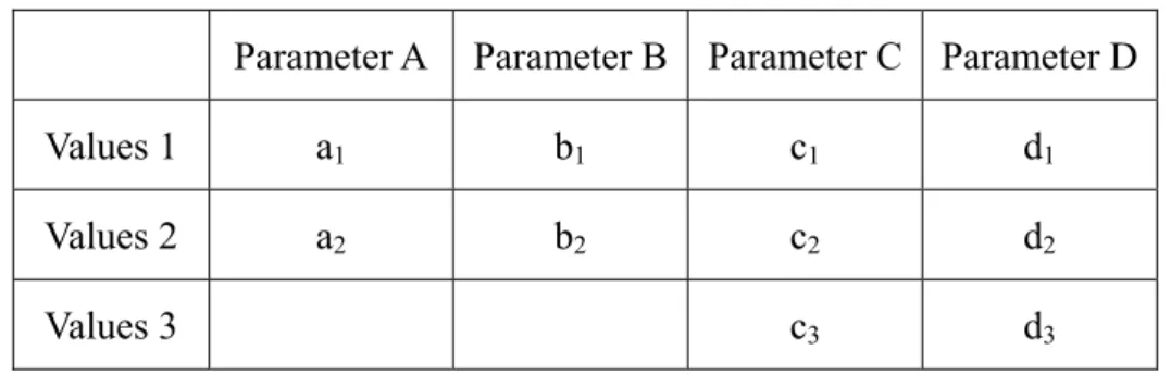
Parameter A Parameter B Parameter C Parameter D

Values 1 a1 b1 c1 d1

Values 2 a2 b2 c2 d2

Values 3 c3 d3

Table 2 Example for IPO strategy

Take Table 2 as an example. There are four parameters A, B, C, and D. A and B are two-valued; C and D are three-valued. Initially, IPO_H works for the first two parameters A and B; four test cases [a1, b1], [a1, b2], [a2, b1], [a2, b2] are generated and Π is empty. Then

parameter C is added to generate twelve uncovered pairs (a1, c1), (a1, c2), (a1, c3), (a2, c1), (a2,

c2), (a2, c3), (b1, c1), (b1, c2), (b1, c3), (b2, c1), (b2, c2) and (b2, c3). Because there are three values

in parameter C, c1, c2, c3 areadded to [a1, b1], [a1, b2], [a2, b1] respectively, and the extended

test cases are [a1, b1, c1], [a1, b2, c2], [a2, b1, c3]. Then these pairs (a1, c1), (b1, c1), (a1, c2), (b2,

c2), (a2, c3), (b1, c3) are removed from Π. To extend [a2, b2], the three possible extensions are

shown as follows.

․ [a2, b2, c1] which covers two uncovered pairs (a2, c1), (b2, c1).

․ [a2, b2, c2] which covers one uncovered pair (a2, c2).

․ [a2, b2, c3] which covers one uncovered pair (b2, c3).

Since [a2, b2, c1] covers the most uncovered pairs. [a2, b2, c1] is chosen as extension [a2,

b2], and (a2, c1) and (b2, c1) are removed from Π.

After IPO_H, there are still four pairs (a1, c3), (a2, c2), (b1, c2) and (b2, c3) in Π. The

test case [a1, *, c3] is generated to cover the pair (a1, c3). Because [a1, *, c3] and (a2, c2) are

generated to cover (a2, c2). The position of parameter B in [a2,*, c2] is *, and the value of

parameter C in (b1, c2) is c2, so the * is changed for b1. The test case [a2,*, c2] is changed to

[a2, b1, c2]. For (b2, c3), the execution process is the same with above, and the test case [a1, *,

c3] is changed to [a1, b2, c3]. The two new test cases are added to the test case set, and there

are six test cases [a1, b1, c1], [a1, b2, c2], [a2, b1, c3], [a2, b2, c1], [a2, b1, c2], [a1, b2, c3] in the test

case set, and no pairs are in Π.

Then parameter D is added, the execution process is the same with the above IPO_H. Finally in IPO_H, the six extended test cases are [a1, b1, c1, d1], [a1, b2, c2, d2], [a2, b1, c3, d3],

[a2, b2, c1, d1], [a1, b2, c3, d3] and [a2, b1, c2, d2], and there are still six pairs (c1, d2), (c1, d3),

(c2, d1), (c2, d3), (c3, d1), (c3, d2) in Π. Because these pairs can not merged together, the six

test cases [*,*, c1, d2], [*,*, c1, d3], [*,*, c2, d1], [*,*, c2, d3], [*,*, c3, d1], [*,*, c3, d2] are

generated and * can be assigned any values of the designated parameter. Finally, the twelve test cases [a1, b1, c1, d1], [a1, b2, c2, d2], [a2, b1, c3, d3], [a2, b2, c1, d1], [a1, b2, c3, d3], [a2, b1, c2,

d2], [*,*, c1, d2], [*,*, c1, d3], [*,*, c2, d1], [*,*, c2, d3], [*,*, c3, d1]and [*,*, c3, d2] are

generated by the IPO, and * can be assigned any values of corresponding parameters.

But in IPO, because each * must be assigned a value of corresponding parameter after each IPO_V, assignment of values to *’s may result that more test case are required to cover all pairs.

For example, there are five two-valued parameters A = {a1, a2}, B = {b1, b2}, C = {c1,

c2}, D = {d1, d2}, E = {e1, e2}. For the first two parameters A and B, four test cases are

generated [a1, b1], [a1, b2], [a2, b1], [a2, b2]. After execution IPO_H for adding parameter C, the

extended test cases are [a1, b1, c1], [a1, b2, c2], [a2, b1, c2], [a2, b2, c1], and no uncovered pairs.

d1], [a1, b2, c2, d2], [a2, b1, c2, d1], [a2, b2, c1, d2], and there are two uncovered pairs (b1, d2) and

(b2, d1). Because (b1, d2) and (b2, d1) can not be merged together, the two test cases [*, b1, *, d2],

[*, b2, *, d1] are generated in IPO_V. Different assignment of values to *’s in [*, b2, *, d1] leads

to different results when parameter E is added:

․ If [*, b2, *, d1] is assigned to become [a2, b2, c1, d1] and [*, b1, *, d2] is assigned to

becomes [a1, b1, c1, d2]. Then parameter E is added, after IPO_H, the six extended test cases

are [a1, b1, c1, d1, e1], [a1, b2, c2, d2, e2], [a2, b1, c2, d1, e2], [a2, b2, c1, d2, e1], [a1, b1, c1, d2, e2] and

[a2, b2, c1, d1, e1], and there is one uncovered pair (c2, e1), therefore, the extra test case [*,*, c2,

*, e1] is need to cover pair (c2, e1).

․ If [*, b2, *, d1] is assigned to become [a2, b2, c2, d1] and [*, b1, *, d2] is assigned to

become [a1, b1, c1, d2]. Then parameter E is added, after IPO_H, the six extended test cases

are [a1, b1, c1, d1, e1], [a1, b2, c2, d2, e2], [a2, b1, c2, d1, e2], [a2, b2, c1, d2, e1], [a1, b1, c1, d2, e2] and

[a2, b2, c2, d1, e1], and no uncovered pairs.

In above example, different assignment of values to *’s in test cases for former processes to cover all pairs lead different number of test cases for five parameters.

Section 2.3 Orthogonal Latin Squares

Another pairwise testing strategy is called “Orthogonal Latin squares” [7][11]. If all parameters have the same number of values, Orthogonal Latin squares can be used to generate optimal test case set. Optimal test case set is the minimum set of test cases which cover all pairs. A Latin square is usually represented by a square matrix as follows:

2 3 1 3 1 2

Values in the column 1 are the values of parameter 1, so are the values in column 2 and column 3, correspondingly. The Latin square has the property that each value in a column or row is distinct.

Assume that there are two matrixes [Aij] and [Bij], if the combined matrix is [Cij] = (Aij,

BBij). For Cij, Cxy, i ≠ x and j ≠ y, if Cij ≠ Cxy, [Aij] and [Bij] are orthogonal. If there are k

parameters, the methodology needs k-2 orthogonal Latin squares. For example, there are four parameters and three values for each parameter, two Orthogonal Latin squares are required and shown as follows:

1 2 3 1 2 3 3 1 2 2 3 1 2 3 1 3 1 2

The following matrix is obtained through superimposing the above matrix. (1, 1) (2, 2) (3, 3)

(3, 2) (1, 3) (2, 1) (2, 3) (3, 1) (1, 2)

The methodology represents the configuration (2, 1, 3, 2): row 2, column 1, entry (3, 2) and the complete set of test configurations is shown as follows:

Configuration number

Parameter1 Parameter2 Parameter3 Parameter4

2 1 2 2 2 3 1 3 3 3 4 2 1 3 2 5 2 2 1 3 6 2 3 2 1 7 3 1 2 3 8 3 2 3 1 9 3 3 1 2 Table 3 Test configurations of orthogonal latin squares

For each row in Table 3, each configuration number means a test case, and the numbers from column 2 to column 5 mean the values’ combination of each test case. Therefore, for four three-valued parameters A = {a1, a2, a3}, B = {b1, b2, b3}, C = {c1, c2, c3} and D = {d1, d2,

d3}. According to Table 3, the optimal nine test cases are [a1, b1, c1, d1], [a1, b2, c2, d2], [a1, b3, c3,

d3], [a2, b1, c3, d2], [a2, b2, c1, d3], [a2, b3, c2, d1], [a3, b1, c2, d3], [a3, b2, c3, d1] and [a3, b3, c1, d2].

However, Orthogonal Latin squares have the following limitation: 1. Orthogonal arrays might not exist.

2. Every parameter must be with the same number of values.

3. |N| means the number of parameters, and |V| means the number of values for each parameter. Orthogonal Latin squares require that |N| isless than |V|+1, and |V| is a power of a prime.

Chapter 3 The IVO Strategy

To solve the disadvantage of IPO (In Parameters Order), in this chapter, a test generation algorithm for pairwise testing called In Values Order (IVO) is described. IVO is improved from the IPO strategy [2] with the execution order of IPO_H and IPO_V. Chapter 3 is organized as follows. Section 3.1 describes the IVO strategy, the simulation results and companion between IVO and IPO. During the simulation, a critical disadvantage of IVO is found, and modified IVO (MIVO) is proposed in section 3.2. Section 3.3 compares with

MIVO and IPO.

3.1 The IVO Strategy

The execution order of IPO is different from that of IVO. For IPO, IPO_H and IPO_V are sequentially operated for each parameter. In IVO, it is assumed that all the input parameters are known and ordered according to the number of values. IVO extends the test cases until all parameters are added, then all uncovered pairs are merged to test cases until all pairs are covered. To explain IVO clearly, the notations are defined as follows.

․P = {P1, P2, … , Pn} is a set of parameters.

․ Vi is the value set of Pi, and |Vi|≥ |Vi+1|.

․νij isthe jth element of Vi.

․PS is the set of uncovered pairs PS = {(a, b) | a ∈ Vi , b ∈ Vj, i≠ j, and (a, b) is

uncovered pair}.

․A test case T= {[a1, a2, … , an] | ai∈ Vi }.

Algorithm: In-Value-Order

00 Begin:

01 for the first two parameters, P1 and P2

02 TS: = {[ v1, v2] | v1∈ V1, v2∈ V2} 03 if n = 2 then stop; 04

∀

∀

09 {

10 extend Tj with νij such that Tj=[ a1, a2, … , ai-1, νij ]

11 and remove (a1, νij), (a2, νij), …,(ai-1, νij) from PS

12 } 13 for |Vi| < j≤ |TS| 14 { 15 can_count = 0 16 Tj=[ a1, a2, … , ai-1] 17 for 1 ≤ k≤ | Vi | 18 {

19 count = | {(az, νik)| z = 1,2,…i-1, (az, νik ) ∈ PS} |

20 if(count > can_count) 21 {

22 can_count = count 23 c = k

24 } 25 }

26 extend Tj with νik, such that Tj=[ a1, a2, … , ai-1, νik ]and remove

27 (a1, νik), (a2, νik), …,(ai-1, νik) from PS

28 } 29 }

30 let TS’ is a test case set, TS’ = Ø 31 ∀ (α, β) ∈ PS, α ∈ Vi, β ∈ Vj

32 {

33 if (∃some test cases T = [a1, a2, … , an], T∈ TS’ that (ai = α, aj 34 = β) or (ai = *, aj = β) or (ai = aj =*))

35 set ai = α, aj = β and remove (α, β) from PS 36 else

37 generate a new test case T = [a1, a2, … , an] in which

38 ∀ z = 1…n, z≠ i, j, az = *, ai = α, aj = β, add T to TS’ 39 remove (α, β) from PS 40 } 41 TS = TS∪ TS’ 42 end

In IVO algorithm, test cases are generated by the first two parameters in line 02. When parameter is introduced in line 06, new generated uncovered pairs are added to PS in line 07. Because parameters are sorted, |TS| must be large than j in line 13. Existing test cases are

extended until all parameters are added from line 08 to line 28. Finally, the uncovered pairs are merged to test cases from line 30 to line 41.

For example, there are four parameters P1 = {ν11, ν12, ν13}, P2 = {ν21, ν22, ν23}, P3 = {ν31,

ν32}and P4 = {ν41, ν42}. Initially in IVO, for the first two parameters P1 and P2, nine test cases [ν11, ν21], [ν11, ν22], [ν11, ν23], [ν12, ν21], [ν12, ν22], [ν12, ν23], [ν13, ν21], [ν13, ν22] and [ν13, ν23] are

generated to TS. Then parameter P3 is added, the twelve uncovered pairs (ν11, ν31), (ν11, ν32),

(ν12, ν31), (ν12, ν32), (ν13, ν31), (ν13, ν32), (ν21, ν31), (ν21, ν32), (ν22, ν31), (ν22, ν32), (ν23, ν31) and (ν23,

ν32) are added to PS. Because there are two values in parameter P3, ν31 andν32 are added to

[ν11, ν21] and [ν11, ν22] respectively. The extended test cases are [ν11, ν21, ν31], [ν11, ν22, ν32], and

the pairs (ν11, ν31), (ν21, ν31), (ν11, ν32) and (ν22, ν32) are removed from PS. To extend [ν11, ν23],

two possible extensions, are shown as follows, are introduced.

․ [ν11, ν23, ν31] which covers uncovered pair (ν23, ν31) in PS

․ [ν11, ν23, ν32] which covers uncovered pair (ν23, ν32) in PS

Both test cases cover only one uncovered pair, [ν11, ν23, ν31] is chosen, and (ν23, ν31) is

removed from PS. For the rest test cases, the extension process is the same as above. Finally, the rest six extended test case are [ν12, ν21, ν32], [ν12, ν22, ν31], [ν12, ν23, ν32], [ν13, ν21, ν31], [ν13, ν22,

ν32] and [ν13, ν23, ν31] and no pairs are left in PS.

When parameter P4 is added, the execution process is the same as above. Nine test cases, [ν11, ν21, ν31, ν41], [ν11, ν22, ν32, ν42], [ν11, ν23, ν31, ν42], [ν12, ν21, ν32, ν41], [ν12, ν22, ν31, ν41], [ν12, ν3, ν32,

ν41], [ν13, ν21, ν31, ν42], [ν13, ν22, ν32, ν41] and [ν13, ν23, ν31, ν41] are extended. However, there is

still one pair (ν12, ν42) left in PS, and test case [ν12, *,*,ν42] is generated to TS in merging

process, and * can be assigned any value of corresponding parameter. The ten test cases are generated by IVO for pairwise testing.

We have implemented a program for simulation of IVO and IPO. The program was written in j2sdk 1.4.2_06 and the computer hardware and software are listed as follows: operation system is windows XP, the cpu is AMD Athon(tm)64 processor(1.81GHz) and the memory is DDR 512MB.

In the program, the input is a set containing numbers of values for each parameter, and the output is all the test cases. Each number in test cases represents the value of the corresponding parameter, i.e., according to the input order, if the first parameter is P1 = {ν11,

ν12, ν13}, ν11 is represented as “1”, ν12 is represented as “2”, and ν13 is represented as “3” in

the first number of each test case, so are the other parameters. The output is composed of three parts, the first part is the extended test cases which are generated by the first two parameters, the second part is the test cases which are generated by merging in the last step and the third is a statement describing the number of uncovered pairs before merging. In the program, the first part and the other parts are separated by a dotted line.

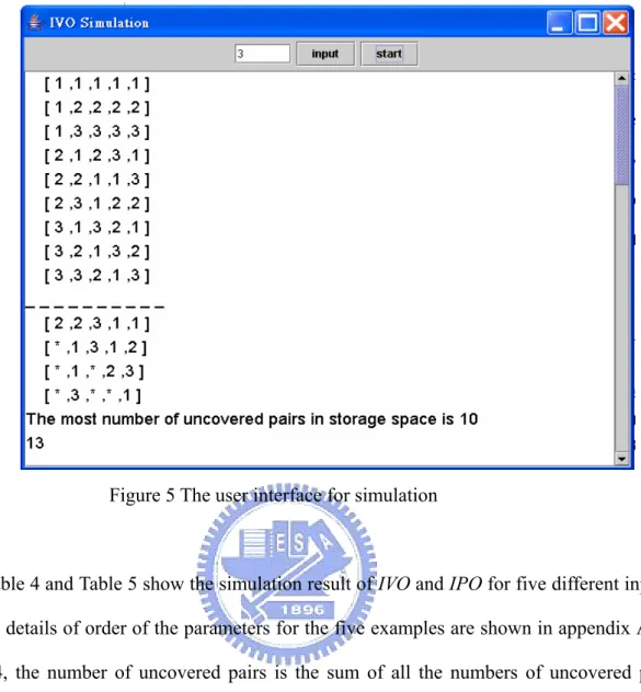
The simulation result for five three-valued parameters is shown in figure 5. All the combination pairs which are generated by two parameters are covered by the thirteen test cases, and * in test cases can be assigned any values of corresponding parameter. Before merging, there are ten uncovered pairs in PS.

Figure 5 The user interface for simulation

Table 4 and Table 5 show the simulation result of IVO and IPO for five different inputs, and the details of order of the parameters for the five examples are shown in appendix A. In Table 4, the number of uncovered pairs is the sum of all the numbers of uncovered pairs before merging.. Obviously, test cases generated by IVO are less than IPO for the first four examples.

Experiment cases: E1: five parameters (5 3-valued).

E2:sevenparameters (1 6-valued, 2 5-valued, 1 4-valued, 2 3-valued, 1 2-valued).

E3: ten parameters (2 7-valued, 2 6-valued, 3 5-valued, 3 4-valued).

E4: twenty-five parameters (5 7-valued, 4 5-valued, 4 4-valued, 6 3-valued, 6

2-valued).

IVO E1 E2 E3 E4 E5

# of test cases 13 33 55 78 131 # of uncovered pairs 10 6 18 132 613 Table 4 Result of the five examples for IVO

IPO E1 E2 E3 E4 E5

# of test cases 14 37 61 86 107 # of uncovered pairs 7 10 45 141 150

Table 5 Result of the five examples for IPO

However, in the fifth example, the number of test cases generated by IVO is more than that by IPO. To clarify such a condition, two experiments, E6 and E7 are designed. E6 is the

case for two-valued of 10, 20, 30 and 40 parameters corresponding. E7 is three-valued

instead. The result for E6 andE7 areshow in Figure 6 and Finger 7 respectively. From the

results of E6 andE7, a critical disadvantage for IVO found. If all input parameters are given

the same number of values, the simulation result of IVO is worse than IPO.

0 5 10 15 20 25 30 35 40 45 10 20 30 40 # of 2-valued parameters # of t es t ca ses IVO IPO Figure 6 Simulation results of IVO and IPO for E6

0 10 20 30 40 50 60 70 80 90 100 110 120 10 20 30 40 # of 3-valued parameters # of test cases IVO IPO

Figure 7 Simulation results of IVO and IPO for E7

In Figure 6, the input is 40 two-valued parameters and the difference in test case size of

IVO and IPO is 26. Furthermore, in Figure 7, the inputs are 40 three-valued parameters, the

difference in test case size between IVO and IPO is 74. With the inputs are n k-valued parameters, larger n and k are, larger the difference in test case size becomes.

The reason is described as follows. Because IVO merges all the uncovered pairs in the last step, the number of test cases can be increased heavily during in this step. If all input parameters are given the same number of values, more uncovered pairs (νij, νkq) are generated

when later parameters Pk are added, 1≤ i≤ k, 1 ≤ j≤ |Vi|, 1 ≤ q≤ |Vk|. The size of test cases in

IVO is larger than that with IPO after uncovered pairs are merged.

Section 3.2 The Modified IVO (MIVO)

To overcome the disadvantage of IVO discussed in above section. We propose another algorithm, called modified IVO (MIVO). MIVO executes mergence once when k new parameters are added. If the number of parameters left is less than k and PS is not empty,

MIVO execute the final mergence in the last step. According to the experiment shown in

Figure 8 and Figure 9, the MIVO gets better result when k is assigned 4.

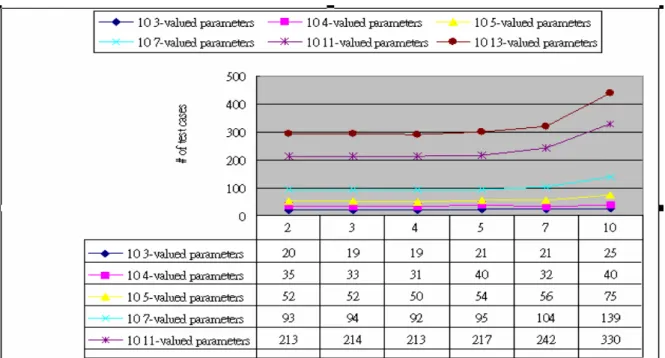
Figure 8 Simulation result for different k’s with 10 n-valued parameters

We analyze above experiments of figure 8 and 9, and find that when k is assigned 2, 3 or 4, the situation of the disadvantage of IVO is not happened, and it gets better result when k is assigned larger number. But when k is assigned 5, the situation of the disadvantage of IVO appears, and the situation is the main reason that the number of test cases for k = 5is larger than that k =4.

MIVO algorithm shows as follows:

Algorithm: Modified In-Value-Order (

)

00 Begin:

01 for the first two parameters, P1 and P2

02 TS: = {[ v1, v2] | v1∈ V1, v2∈ V2} 03 if n = 2 then stop; 04

∀

∀

08 for 1 ≤ j ≤ |V i| that Tj=[ a1, a2, … , ai-1]

09 {

10 extend Tj with νij such that Tj=[ a1, a2, … , ai-1, νij]

11 and remove (a1, νij), (a2, νij), …,(ai-1, νij)from PS

12 }

13 for |V i| < j≤ |TS|

14 {

15 can_count = 0 16 Tj=[ a1, a2, … , ai-1]

17 for 1 ≤ k≤ | Vi |

18 {

19 count = | {(az, νik)| z = 1,2,…i-1, (az, νik )∈ PS} |

20 if(count > can_count) 21 { 22 can_count = count 23 c = k 24 } 25 }

26 extend Tj with νik such that Tj=[ a1, a2, … , ai-1, νik]

27 and remove (a1, νik), (a2, νik), …,(ai-1, νik) from PS

28 }

29 if (i mod 4 = 0) 30 {

31 let TS’ is a test case set, TS’ = Ø 32 ∀ (α, β) _{∈ PS, α ∈ V}i, β ∈ Vj

33 {

34 if (∃_{some test cases} T = [a1, a2, … , an], T∈ TS’

35 that(ai = α, aj = β) or (ai = *, aj = β) or(ai = aj = *)) 36 set ai = α, aj = β and remove (α, β) from PS 37 else

38 generate a new test case T = [a1, a2, … , an] in

39 which ∀ z = 1…n, z≠ i, j, az = *, ai = α, aj = 40 β, add T to TS, remove (α, β) from PS

41 }

42 if(PS is empty)

43 * is assigned any values of corresponding 44 parameter 45 TS = TS∪ TS’ 46 } 47 } 48 TS’ = Ø 49 ∀ (α, β) _{∈ PS, α ∈ V}i, β ∈ Vj 50 {

51 if (∃_{some test cases} T = [a1, a2, … , an], T∈ TS’ that (ai = 52 α, aj = β) or (ai = *, aj = β) or (ai = aj =*))

53 set ai = α, aj = β and remove (α, β) from PS 54 else

55 generate a new test case T = [a1, a2, … , an] in which

56 ∀ z = 1…n, z≠ i, j, az = *, ai = α, aj = β, add T to TS’ 57 remove (α, β) from PS 58 } 59 TS = TS ∪TS’ 60 end

In MIVO algorithm, test cases are generated by the first two parameters in line 2. When parameter is introduced in line 6, the generated uncovered pairs are put in PS in line 7. The extension for existing test cases is similar to previous algorithm, except that each mergence is done for adding every 4 new parameters from line 8 to line 46. Finally, the rest uncovered

pairs are merged to test cases from line 48 to line59.

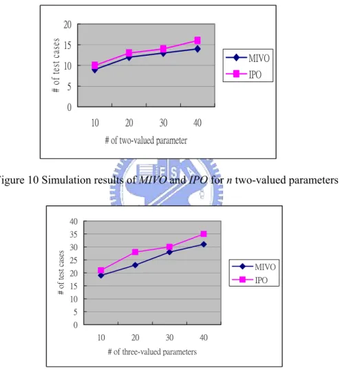
The extension results of MIVO for E6 and E7 are shown in Figure 10 and Figure 11.

Obviously, MIVO have great improvement in the number of test cases of MIVO for parameters with the same number of values.

0 5 10 15 20 10 20 30 40 # of two-valued parameter # of t es t cas es MIVO IPO

Figure 10 Simulation results of MIVO and IPO for n two-valued parameters

0 5 10 15 20 25 30 35 40 10 20 30 40 # of three-valued parameters # of t es t cas es MIVO IPO

Figure 11 Simulation results of MIVO and IPO for n three-valued parameters

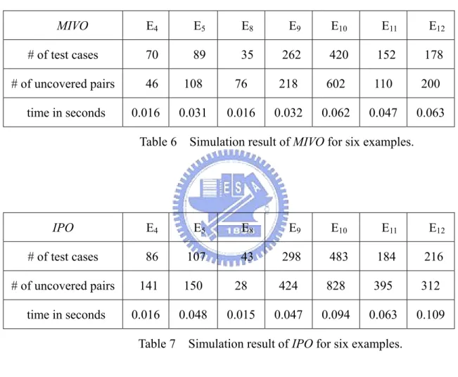
Table 6, 7 and 8 show the simulation results of MIVO, IPO, and IVO for the examples E4, E5, E6, E7, E8 and E9, the parameters input order is recorded in Appendix A.

Experiment cases:

E9: twenty-five parameters (6 13-valued, 5 11-valued, 7 9-valued, 7 7-valued).

E10: thirty parameters (10 15-valued, 10 13-valued, 10 10-valued).

E11: forty-three parameters (5 10-valued, 6 8-valued, 8 6-valued, 4 5-valued, 6

4-valued, 6 3-valued, 8 2-valued).

E12: fifty-four parameters (6 10-valued, 6 9-valued, 6 8-valued, 6 7-valued, 6

6-valued, 6 5-valued, 6 4-valued, 6 3-valued, 6 2-valued).

MIVO E4 E5 E8 E9 E10 E11 E12

# of test cases 70 89 35 262 420 152 178 # of uncovered pairs 46 108 76 218 602 110 200

time in seconds 0.016 0.031 0.016 0.032 0.062 0.047 0.063 Table 6 Simulation result of MIVO for six examples.

IPO E4 E5 E8 E9 E10 E11 E12

# of test cases 86 107 43 298 483 184 216 # of uncovered pairs 141 150 28 424 828 395 312

time in seconds 0.016 0.048 0.015 0.047 0.094 0.063 0.109 Table 7 Simulation result of IPO for six examples.

IVO E4 E5 E8 E9 E10 E11 E13

# of test cases 78 131 64 419 1040 221 385 # of uncovered pairs 132 613 432 1770 8673 639 3058 time in seconds 0.016 0.031 0.015 0.016 0.157 0.031 0.046

Chapter 4 Extending A Test Case Set Based On Duplication

In the chapter, we discuss an algorithm to duplicate the data pairs. In the algorithm, test cases can be quickly extended under some constraints. Section 4.1 introduces the duplicate algorithm. Section 4.2 introduces a pairwise graph model. Section 4.3 proves the correctness of the duplicate algorithm and discusses influence when adding a k-valued parameter to a test case set which covers pairwise perfectly for n.

Section 4.1 An Extension Algorithm With Duplicate Technique

Definition 4.1. (pairwise perfectly coverage): A test case set TS is claimed to cover

pairwise perfectly for n, when there are n+1 parameters, each of which has n

values and all pairs appears distinctly in TS.

For example, given three three-valued parameters P1 = {ν11, ν12, ν13}, P2 = {ν21, ν22, ν23}

and P3 = {ν31, ν32, ν33}, and the test case set TS ={[ν11, ν21, ν31][ν11, ν22, ν32][ν11, ν23, ν33][ν12, ν21,

ν32][ν12, ν22, ν33][ν12, ν23, ν31][ν13, ν21, ν33][ν13, ν22, ν31][ν13, ν23, ν32]} which cover all pairs without

repetition. Thus, TS covers pairwise perfectly.

Consider the system which has n+1 parameters, and each parameter contains n distinct values, n≥ 1. The testing data need n2(n) + n2(n-1) + … + n2*1 = n2 [(n) + (n-1) + … +1] =

n3(n+1)/2 pairs at most. Let each test case have n+1 values and each pair be generated by choosing any two values of them. Each of these test cases covers n(n+1)/2 pairs at most and the least number of test cases is [n3 (n+1)/2]/ n(n+1)/2 = n2.

Definition 4.2. (block): Let a test case set TS cover pairwise perfectly for n. A block is a set containing n test cases which have the same value of parameter P1. A block BB

= {Ti | 1≤ i≤ n, Ti is a test case and Ti has the same value of P1}.

Proposition 4.1: Let a test case set TS cover pairwise perfectly for n. Each test case can be assigned to some block and the TS can be divided into n different blocks

Proof: Because TS covers pairwise perfectly for n, all combination pairs are in TS. Consider v11 and v2i, 1≤ i≤ n. The n pairs (v11, v21), (v11, v22), …, (v11, v2n) are in TS.

∀

there are n test cases whose first value is v1j, thus TS can be divided into n different blocks.□

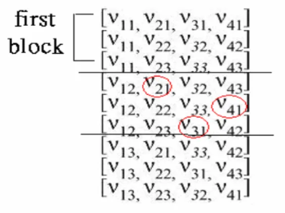
Let a test case set TS cover pairwise perfectly for n. According to proposition 4.1, there exist a block in which all test cases for P1 have the same value, and these test cases can be

formed as [v1i, v2j, v3j, … , v(n+1)j], 1≤ i, j≤ n. Such a block is called the first block, and

W.L.O.G., in following sections, the first block is used to prove or clarify the property for the duplicate algorithm.

Figure 12 is an example that the test case set TS covers pairwise perfectly for 3 and test cases are divided into three blocks.

There’re three properties for a test case set TS which covers pairwise perfectly for n. Property 1.

∀

∉

Property 1 holds because for any two test cases Ta and Tb in the same block, if vij ∈ Ta, vij∈Tb, 1<i≤ n+1 and 1≤ j≤ n, the pair (v1k, vij), 1≤ k≤ n, appears repeatedly,

Property 2.

∀

∉

Property 2 holds because

∀

appears repeatedly with test cases in the first block.

The Duplicate Algorithm:

Input: A test case set TS covers pairwise perfectly for n, and m n-valued parameters waiting to be extended, where 1≤ m≤ n+1.

00 Begin:

01

∀

02

∀

03

∀

04 if (νij∈ Ta) extend Ta by adding v(n+i+1)j

05 End

The extended test case set loses n(n-1) pairs for each new added parameter. This is proved in section 4.3. Take figure 13 as an example, there are four three-valued parameter P1 = {ν11, ν12, ν13}, P2 = {ν21, ν22, ν23}, P3 = {ν31, ν32, ν33} and P4 = {ν41, ν42, ν43} and the test case

{ν61, ν62, ν63}, P7 = {ν71, ν72, ν73} and P8 = {ν81, ν82, ν83} being added, each test cases are

extended according to the duplicate algorithm and the extension result is shown in figure 13.

Figure 13 Example of the duplicate algorithm

After executing the duplicate algorithm, there are some uncovered pairs, and the form of uncovered pairs must be (v i1, v(n+i+1)2), (v i1,v (n+i+1)3),…, (v i1,v (n+i+1)n),…,(v in, v (n+i+1)1),

(vin, v(n+i+1)(n-1)), 1≤ i≤ n+1. Because n*(n-1) pairs are lost for adding each new parameter,

n*(n-1) test cases are need to cover these uncovered pairs. The test cases generation

algorithm is as follows:

Incremental -Test case - generation algorithm (ITG)

Input: The input is a TS which is generated by executing the duplicate algorithm, and the input to the duplicate algorithm is a test case set which covers pairwise perfect for n, and m n-valued parameters are waited to be extended, 1≤ m≤ n+1. 00 Begin

01

∀

03

∀

05 νij is the jth value of parameter Pi, 1≤ j≤ |Vi|.

06 generate a test case [v1i, v2i,…, v(n+1)i, v(n+2)j, v(n+3)j,…,v (n+m+1)j] to

07 TS 08 }

09 } 10 End

Section 4.2 The Pairwise Graph Model.

To assist the proof of the duplicate algorithm, the pairwise graph model is introduced first.

Definition 4.3. (pairwise graph model): A pairwise graph is an undirected graph G = (N, A). N is a set of nodes, of which a node is named as nij, 1≤ i,j≤ n, and nij

represents the jth value of Pi. For any arc e ∈ A, e connects nij and n(i+1)k , i≥ 1, 1≤ j≤

|Vi|, 1≤ k≤ |Vi+1|.

Definition 4.4. (complete path): Given n parameters, a complete path is defined as a path in a pairwise graph that starts from n1i and ends in nnj,1≤ i≤ |V1|, 1≤ j≤ |Vn|. In a

Figure 14. Pairwise graph

Consider the example shown above, where three three-valued parameters are P1 = {ν11,

ν12, ν13}, P2 = {ν21, ν22, ν23}, P3 = {ν31, ν32, ν33}. In the pairwise graph, N = {n11, n12, n13, n21,

n22, n23, n31, n32, n33} and path 1 consists of [v11, v21, v31] and path 2 consists of [v12, v21, v32],

and both paths are complete paths.

If a test case set covers pairwise perfectly for n, its corresponding pairwise graph has the following properties:

Property 1. For all complete paths, each arc is walked through once.

Property 1 holds because for each arc, if the arc is walked through twice, the corresponding pair appears twice in the test case set.

Property 2. For any paths, the pairs of the start and end nodes for any path are different to other paths that of another path.

Property 2 holds because for all paths, if the pair of the start and end nodes for any path is the same with another path, the corresponding pair appears twice in the test case set.

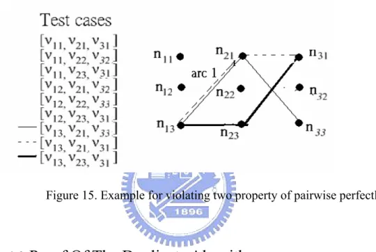
Take figure 15 as an example, there are three three-valued parameter, P1 = {ν11, ν12, ν13},

P2 = {ν21, ν22, ν23} and P3 = {ν31, ν32, ν33}. Consider the paths for [ν13, v21, v33], [ν13, v21, v31]

and [ν13, v23, v31]. The paths corresponding to [ν13, v21, v33] and [ν13, v21, v31] go through arc 1,

and the property 1 is violated. For [ν13, v21, v31] and [ν13, v23, v31], the pairs of start and end

node are the same. Therefore the property 2 is violated.

Figure 15. Example for violating two property of pairwise perfectly

Section 4.3

Proof Of The Duplicate Algorithm

To prove the correctness of the duplicate algorithm, some propositions are introduced firstly.

Definition 4.5. (value independent): If all the pairs generated for two parameters Pi

and Pj are distinct in the test case set TS, Pi and Pj are claimed "value independent"

in the TS.

For example, there are three parameters P1 = {ν11, ν12, ν13}, P2 = {ν21, ν22,} and P3 = {ν31,

[ν13, ν21, ν31], [ν13, ν22, ν32]}. Each pair (ν1i, ν3j) is distinct in the TS, 1≤ i, j≤ 3, and parameter

P1 and P3 are value independent in the TS. Because (ν21, ν31) and (ν22, ν32) appear twice,

parameter P2 and P3 are not value independent in the TS.

To prove the following propositions, an Incremental-TS-extension (ITE) method is introduced. The ITE method is used to duplicate the permutation of pairs for a parameter in the test case set.

Incremental- TS -extension (ITE) method

Input: A TS covers all pairs which are generated by the k parameters. Let the parameter Pi be one of the k parameters, and Pk+1 is a new parameter which is waited

to be added to TS, |Vi|≤ |Vk+1|.

00 Begin

01

∀

03 νij is the jth value of parameter Pi, 1≤ j≤ |Vi|.

04 if(νij∈ Ta)

05 extend Ta by adding ν(k+1)j

06 } 07 End

Proposition 4.2: Let two parameters Pi and Pj be value independent in the test case

set TS, 1≤ i, j≤ k. When a new parameter Pk+1 is added, |Vk+1|≥ |Vi|. After executing

Pk+1 are also value independent in the extended test case set.

Proof: Assume that Pi and Pj are value independent in the extended test case set, but

parameters Pj and Pk+1 are not value independent. There are some pairs (vjm, v(k+1)n) where 1≤

m≤ |Vj|, 1≤ n≤ |Vk+1|, which appear repeatedly in the extended test case set. The pairs (vin, vjm)

also appear repeatedly in the extended test case set, and parameters Pi and Pj are not value

independent. That is a contradiction, and therefore parameters Pj and Pk+1 are value

independent.□

Proposition 4.3: Let the test case set TS cover pairwise perfectly for n. For any two test cases in different blocks, there is only one value in common.

Proof:

∀

pair generated by the two values appears twice and TS doesn’t cover pairwise perfectly for n. That is a contradiction.

Because test cases are divided into blocks according to the value of parameter P1, the

value of P1 is different for any twotest cases in different block. Consider the values of

parameter P2 to Pn+1, because TS cover pairwise perfectly for n, all values appear once in a

block.

∀

can be found that vkl is in Tb, i≠ j. For any two test cases in different blocks, there is only one variable that has the same value.

Proposition 4.4: Let the test case set TS cover pairwise perfectly for n. If an n-valued parameter is added, the extended test case set lose n(n-1) pairs at least without increasing the number of test cases.

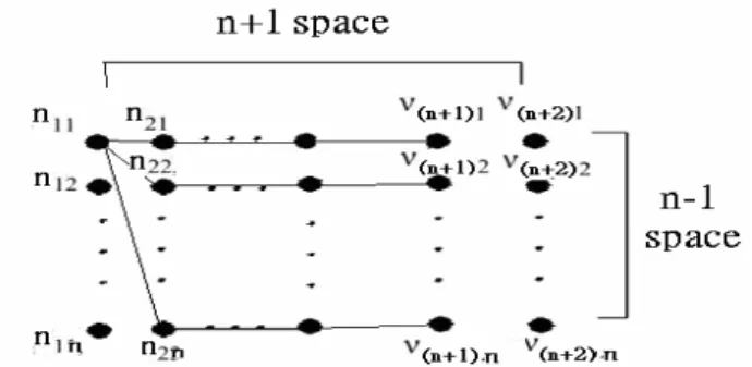
Proof: W.L.O.G, assume that the first value is v11 foreach test case in the first block and

figure 16 is the corresponding pairwise graph. When parameter Pn+2 is added, two cases are

discussed as follows. In case 1, all test cases in the first block are extended by adding n values of Vn+2. In case 2, test cases in the first block are extended by adding j values of Vn+2,

0≤ j≤ n-1.

Case1: The ith test case in the first block is extended by adding v(n+2)j, 1 ≤ i, j≤ n. There

are n+1 space for n+2 parameters and n-1 space for n values in pairwise graph. For each complete path except the first block, if i = j and the last node is n(n+2)k, the node nik can be

found in the same complete path and is shown in the case 1 of figure 17. The pair (vik, v(n+2)k)

appears repeatedly with the pair in the first block. If i≠ j, the proof is the same with above and the repeated pairs become (vik, v(n+2)l), k≠ l, and the corresponding graph is the case2 of

Figure 17.

∀

the extended test case set loses n(n-1) pairs at least.

Case2: Test cases in the first block are extended by adding j values of Vn+2, 0≤ j≤ n-1. If

all test cases in the first block are extended, there are n-j repeated pairs in the first block. According to proposition 4.3, there is one same value for any two test cases in different blocks. For the remainder n(n-1) test cases, only n-j test cases have no repeated pairs, and each of the n2-2n+j test cases has least one repeated pair, so the total lost pairs are n2-2*n+ j+

Figure 16 Pairwise graph for n+2 n-valued parameters

Figure 17 Form of the Repeated covered pairs

Proof of the correctness of the Duplicate Algorithm: A test case set TS covers pairwise perfectly for n. m n-valued new parameters are waited to be extended, 1≤

m≤ n+1. After extension by using duplicate algorithm, the test case set TS loses n(n-1) pairs for adding a new parameter and the test cases set has the most pairwise

coverage than other test case sets with the same size.

Proof: Because the test case set TS covers pairwise perfectly for n, any two parameters between P1 and Pn+1 are value independent in TS. According to proposition 4.2, the

parameter Pn+i+1 is value independent with former parameters except parameter Pi, 1≤ i≤ m,

and the number of repeated pairs generated by Pi and Pn+i+1 is n (n-1). According to

Therefore, the TS extended by the duplicate algorithm still cover the most pairs without increasing number of test cases.□

The advantage for using the duplicate method is when new parameters are added, the test cases can be extended quickly. The duplicate method reduces large time in extension and retains high coverage rate.v1i,

Finally, some situations are discussed as follows. Let the test case set TS cover pairwise perfectly for n. There are k*n(n+1) new pairs are generated when a k-valued parameter is added, k≠ n. Without increasing the number of test cases, how many pairs are lost at least after extension for k< n, n< k≤ n2 and k>n2?

k< n: the least number of lost pairs is zero. There are k*n(n+1) new pairs are generated

when adding a new parameter and the extended test cases can cover n2(n+1) new pairs at most, so the least number of lost pairs is zero.

n< k≤ n2: the least number of lost pairs is n(n+1)(k-n)+n2-k. If there are no repeated pairs in the extended test cases, the extended test cases cover n2(n+1) new generated pairs. Because k≤ n2, repeated pairs are not found in only k extended test cases, and the remainder

n2- k test cases have more than one repeated pair. The reason is same with the case 2 of proposition 4.4, so the number of lost pairs is n(n+1)k-n2(n+1) + n2-k.

k>n2: the least number of lost pairs is n(n+1)(k-n). If there are no repeated pairs in the extended test cases, the extended test cases cover most n2(n+1) new pairs, so the number of lost pairs is n(n+1)k-n2(n+1) = n(n+1)(k-n).

Chpater 5 Conclusion and Future Work

MIVO is more effective.

The duplicate algorithm is also introduced and clearly proved in this paper. Using the duplicate algorithm, the extended test cases retain high pair’s coverage. With the advantage of using the algorithm is that test cases can be easily extended and large amount of computing time for extension can be saved

Much works also remains to be done to validate the result of MIVO. In the future, we hope that MIVO testing strategy can be implemented to test real software systemes and more empirical results are gathered to confirm the usefulness of MIVO.

References

[1] Y.Lei and K.C. Tai, “In-Parameter-Order: A Test Generation Strategy for Pairwise Testing,” Technical Report TR-2001-03, Dept. of Computer Science, North Carolina State Univ., Raleigh, North Carolina, May, 2001.

[2] Y.Lei and K.C. Tai. ”A Test Generation Strategy for Pairwise Testing”, IEEE Trans of Software Engineering, Vol 28, NO.1, Jan 2002.

[3] D.M. Cohen, S.R. Dalal, M.L. Fredman, and G.C. Patton, “The AETG System: An Approach to Testing Based on Combinational Design,” IEEE Trans. Software Eng., vol. 23, no.7, pp.437-443, July 1997.

[4]D. M. Cohen, S. R. Dalal, M.L. Fredman, and G.C. Patton, “The combinatorial design approach to automatic test generation.” IEEE Software, pages 83-87, September 1996.

[5]Glenford J. Myers, “The Art of Software Testing,” Senior Staff Member, IBM Systems Research Institute, Lecturer in Computer Science, Polytechinic Institute of New York.

[6]Roger S. Pressman, Ph.D.,”Software Engineering: A Practitioner’s Approach”, Sixth Edition. 2005.

[7]R.Mandl, ”Orthogonal Latin squares: An application of experiment design to compiler testing”, Communications of the ACM, Vol. 28 NO. 10(October 1985) pp.1054-1058.

[8]Dennis. Jeffrey and Neelam Gupta,” Test Case Prioritization Using Relevant Slices”, Annual International Computer Software and Applications Conference (COMPSAC’06), IEEE, 2006.

[9] Renee C. Bryce and Charles J. Colbourn, “Test Prioritization for Pairwise Interaction Coverage”, A-MOST’05, May 15-21,2005, St. Louis, Missouri, USA.

Copyright 2005 ACM.

[10] James A. Jones and Mary Jean Harrold, “Test-Suite Reduction and Prioritization for Modified Condition/ Decision Coverage”, IEEE Trans., Software Eng ., 2003.

[11]Soumen Maity and Amiya Nayak “Improved Test Generation Algorithms for Pair-wise Testing” 2005 IEEE, Software Reliability Engineering.

[12]S. Elbaum, A. Malishevsky, and G. Rothermel, ”Prioritizing Test Cases for Regression Testing,” Proc. ACM Software Testing and Analysis, pp. 102-112, Aug. 2000.

[13] D. M. Cohen, S. R. Dalal, A. Kajla, and G.C. Patton, “The automatic Efficient Test Generator (AETG) System”, Proceedings of the 5th IEEE International Symposium on Software Reliability Engineering, pages 303-309, Nov. 1994

[14] D. M. Cohen, S. R. Dalal, J. Parelius, and G.C. Patton, “Combination Design Approach to Automatic Test Generation”, IEEE Software, 13: pages 83-88,1996

Appendix A

The input order of the example for simulation E1: five parameters (5 3-valued).

E2: sevenparameters (5, 6, 3, 2, 3, 4, 5)

E3: ten parameters (7, 4, 6, 5, 7, 5, 5, 6, 4, 4)

E4: twenty-five parameters (3, 3, 4 ,7, 2, 5, 4, 2, 7, 3, 5, 2, 2, 2, 4, 3 ,3 ,7 ,2 ,4 ,3, 5, 5, 7, 7)

E5: forty parameters (5, 4, 2, 3, 7, 2, 4, 4, 5, 3, 2, 2, 5, 7, 4,7, 3,3,4,5, 3,4,5,2, 2,7,2,3,

7,7,5,4,7,2,3,3,4,5,5,7)

E8: twenty parameters (20 4-valued).

E9: twenty-five parameters (11, 11, 13, 7, 9, 9, 13, 13, 11, 7, 7, 7, 13, 11, 9, 7, 9, 7, 13, 11, 7, 9, 9, 13, 7, 9) E10: thirty parameters(10, 13,10,15,13,13,10, 15,13,15,10,10,15,13,13,10, 15,15,10,13, 10,15, 13,10,15,10,13, 13,15,15) E11: forty-three parameters (6, 5, 5, 4, 3, 2, 6, 8, 4, 2, 6, 5, 3, 3, 10, 4, 2, 8, 2, 2, 6, 8, 3, 10, 2, 6, 6 , 5, 4, 4, 10, 2, 8, 8, 6, 4, 10, 2, 3, 3, 6, 8, 10). E12: fifty-four parameters(6, 9, 2, 10, 3, 5, 5, 7, 6, 3, 2, 4, 4, 9, 8, 2, 10, 7, 3, 9, 5, 5, 8, 4, 8, 10, 6, 3, 3, 8, 9, 5, 7, 6, 7, 5, 3, 10, 10, 2, 8, 6, 7, 4, 7, 6, 8, 4, 10, 2, 2, 9, 4, 9).