以貝氏方法構建與求解路徑基礎之時變交通指派模式

(1)

國

立

交

通

大

學

運輸科技與管理學系

博士論文

以貝氏方法構建與求解

路徑基礎之時變交通指派模式

Time-varying Path-based Traffic Assignment

Using Bayesian Approach

研究生：藍健綸

指導教授：卓訓榮教授

周幼珍副教授

(2)

以貝氏方法構建與求解路徑基礎之時變交通指派模式

學生：藍健綸

指導教授：卓訓榮

周幼珍

國立交通大學運輸科技與管理學系博士班

摘要

現今之交通運輸系統不再是以「大規模的建設」來解決所有的運

輸問題，而是朝向一個更細緻化、對環境更友善且能夠永續經營的

方式。智慧型運輸系統，整合了電子、通訊、資訊處理等技術，希

望能夠透過有效之管理方式來減少交通擁擠狀況。於智慧型運輸系

統當中的先進交通管理系統，則需要即時交通狀況之資訊，才能據

以進行分析與控制。因此，本研究發展一路徑基礎之動態交通量指

派模式，並據此推估路網現況。

大多數動態交通量指派之研究，均專注於探討使用者均衡或系統

最佳狀態。但路網現況是否滿足使用者均衡，仍有許多學者存疑。

是故，本研究不以使用者均衡指觀點描述交通量指派問題，而是透

過線性動態系統構建路徑基礎之動態交通量指派模式。由最基礎之

非時變且不考慮旅行時間之模式，逐漸放鬆成為時變且考量旅行時

間之模式。過去針對此種動態系統所構建之模式，大多需要歷史之

起迄流量資訊、路徑選擇矩陣或狀態轉移矩陣；但在現實環境中，

這些資訊不一定能夠順利取得。本研究透過貝氏方法以及卡門濾波

兩者之結合，放鬆上述之假設條件，並且提出一整合型演算法求解

此模式。為確認此演算法之收斂，本研究亦提出一平行數列收斂性

確認方式，作為此演算法之收斂停止條件。由於此演算法需要大量

之計算，為增進計算效率，本研究將此演算法以通訊量最小化的目

標進行平行化，並執行於平行電腦上。透過真實路網流量資訊，本

研究得以驗證此模式之估計與執行效率。

(3)

ii

Time-varying Path-based Traffic Assignment Using

Bayesian Approach

Student: Chien-Lun Lan

Advisors: Hsun-Jung Cho

Yow-Jen Jou

Department of Transportation Technology and Management

National Chiao Tung University

ABSTRACT

Transportation system nowadays is no longer “extraordinary

construction” but becomes more elegant, environmental-friendly, and

sustainable. Intelligent Transportation System (ITS) integrates the

telecommunications, automation, electronics, and information processing

system, is considered possessing the potential to solve the traffic

congestion problem. Advanced Traffic Management Systems (ATMS),

requires real-time traffic condition, is one of the key issues of ITS.

Therefore, we suggest a path-based traffic assignment model to describe

the network flow status.

Most existing research works on dynamic traffic assignment focus

on the user-equilibrium or system optimal. Nevertheless, the existence of

such assumption in real world network is questionable to many

researchers. An approach without these assumptions while keeping the

basic traffic relationship might be useful facing the disequilibria issue.

Therefore, we model the dynamic traffic assignment problem with

dynamic system approach. Existing researches with this approach

usually assume the prior information of O-D matrix, link-proportion

matrix, or state transition matrix. In this paper, we relax such assumption

by combining Gibbs sampler and Kalman filter in a state space model. A

solution algorithm with parallel chain convergence control is proposed

and implemented. To enhance its efficiency, a parallel structure is

suggested with efficiency and speedup demonstrated using PC-cluster.

(4)

List of Figures

Figure 1.1 Overview of the dissertation ... 1

Figure 2.1 Typical Link Performance Function ta(xa) ... 8

Figure 2.2 A possible shape of link exit function ... 13

Figure 3.1 The solution framework of state space model ... 33

Figure 3.2 The solution framework of time-invariant coefficient state space model considering link travel time ... 39

Figure 4.1 The solution framework of time-varying coefficient state space model considering link travel time ... 46

Figure 5.1 Example 1 of four parallel chains ... 50

Figure 5.2 Example 2 of four parallel chains ... 51

Figure 5.3 Example of eight parallel chains ... 51

Figure 5.4 The parallel computation structure ... 53

Figure 5.5 Speedups and efficiencies for the parallel computing ... 54

Figure 6.1 The MRT test network ... 55

Figure 6.2 The comparison of real and estimated data on MRT network by time-invariant coefficient model. ... 58

Figure 6.3 The comparison of real and estimated data on MRT network by time-invariant coefficient model. ... 60

Figure 6.4 The comparison of real, estimated, and predicted path flows on MRT network by time-varying coefficient model with 9 states in a horizon period ... 62

(8)

Figure 6.6 The comparison of real and estimated data on freeway network by time-invariant coefficient model considering travel time effect. ... 69 Figure 6.7 The comparison of real and estimated data on freeway network by

time-varying coefficient model considering travel time effect. ... 73 Figure 6.8 The result comparison with predetermined transition matrix ... 75 Figure 7.1 Roadmap of future researching topics ... 81

(9)

viii

List of Tables

Table 3.1 Notations of time-invariant state space model ... 21

Table 3.2 Principal dynamic system models ... 22

Table 3.3 Notations of time-invariant state space model considering link travel time ... 33

Table 4.1 Notations of time-varying state space model ... 40

Table 6.1 Path set of example MRT network ... 55

Table 6.2 Time-dependent link flows of MRT network ... 56

Table 6.3 An example of rolling horizon estimation ... 60

(10)

Chapter 1 Introduction

Transportation systems play an important role in the development of a country. It provides a source of mobility by the extensive network of freeways, expressways, and streets. In recent years, the mobility has been greatly obstructed by delays due to the congestion on overloaded transportation networks. The economy suffers a great loss owing to the worsening of traffic congestion. Dynamic traffic management is an efficient tool to control traffic congestion, and this tool requires information of traffic states. Traditional static methods are not suitable for this dynamic traffic management task. Therefore, a new assignment model that gives proper information to fulfill the need is worth to develop. In the introduction, we will discuss motivations, objectives, overview, and contributions of this research.

1.1 Research Motivations

Transportation system nowadays is no longer “extraordinary construction” but becomes more elegant, environmental-friendly, and sustainable. Building new highways is no longer a suitable option for every situation due to the prohibitively high costs involved, as well as social, political and environmental concerns. Intelligent Transportation System (ITS) integrates the telecommunications, automation, electronics, and information processing system, is considered possessing the potential to solve the traffic congestion problem. Advanced Traffic Management Systems (ATMS) is one of the key issues of ITS. Proper information, i.e. link flows,

(11)

2

and origin-destination (O-D) demands, is a requirement to management the traffic system effectively. Information of can be obtained by comprehensive deployment of surveillance system, but the costs of extensive installation is nearly unbearable. Hence, estimate these precious information with reasonable amount of detectors is a research that worth some attention.

1.2 Research Objectives

The fundamental objective of this dissertation is to address a dynamic stochastic path-based assignment model. Utilizing link traffic counts, this model can give an overview of the network. Existing research works concerning this problem usually assume the existence of user-equilibrium or system optimal condition. Nevertheless, the existence of such assumption in real world network is questionable (Friesz, Bernstein, Mehta, Tobin and Ganhalizadeh, 1994; Friesz and Shah, 2001). An approach without these assumptions while keeping the basic traffic relationship (i.e., path-link incidence matrix) might be useful facing the disequilibria issue. A statistical approach will be introduced in this dissertation to relax such behavioral assumption. Issues concerning the objective include:

1. Development of a path-base assignment model without user behavior

assumptions.

2. Modeling the path-base assignment problem with linear time-varying

coefficient dynamic system, that addresses the time-dependent path flows.

3. Present a solution algorithm with parallel computing capability to improve

(12)

4. Demonstrate the path-base assignment model with real network data.

1.3 Research Overview

This dissertation is organized as follows. First, the introduction chapter gives an overview of the motivation, research objectives, and overview of this dissertation. Second, a literature review of related researches in the relevant areas. The literature review chapter concerns about topics include: i) Static Trip distribution models and ii) dynamic trip assignment models.

A path-base assignment model with time-invariant coefficient dynamic system is proposed in chapter 3. Essential algorithms for solving this model, including Kalman Filter and Gibbs Sampler, are discussed. Macroscopic traffic flow model that represent the link dynamics is introduced along with finite difference scheme that solve it numerically. In chapter 4, a time-varying coefficient dynamic model with rolling horizon structure addressing the transition matrix is introduced.

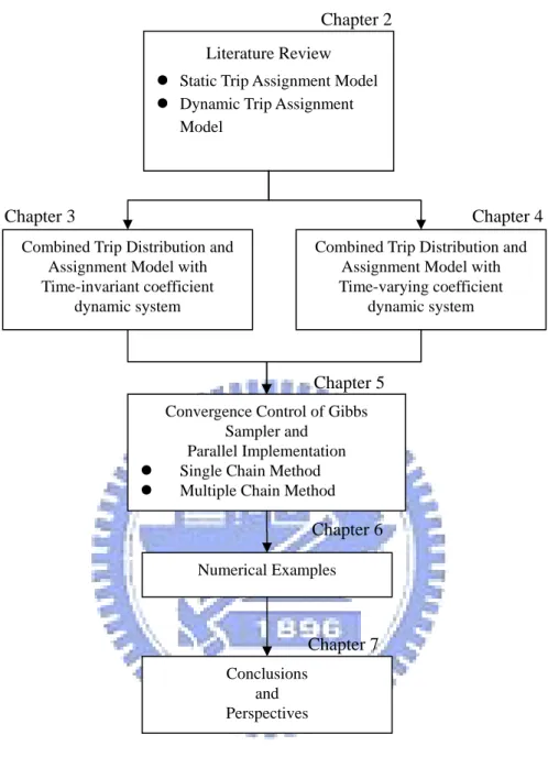
Gibbs sampler, a powerful simulation method, draws values of a random variable from a sequence of distribution that converges to a desired target distribution. If used naively, it might give a misleading answer. Therefore, convergence assessments of the Gibbs Sampler with single chain method and multiple chain method are discussed in chapter 5. Gibbs sampler requires tremendous iteration during computation. To make the model more suitable for real-time use, parallel computing is also introduced in chapter 5 to increase the performance. Numerical examples with real data are also discussed in chapter 6. The last chapter presents the conclusions and perspectives of this study. The overview of the dissertation are illustrated in Figure 1.1.

(13)

4

Figure 1.1 Overview of the dissertation.

1.4 Research Contributions

The principal contributions of this study are as follows:

1. Development of a dynamic path-base assignment model with no user

behavior assumptions.

Literature Review z Static Trip Assignment Model z Dynamic Trip Assignment

Model

Combined Trip Distribution and Assignment Model with Time-invariant coefficient

dynamic system

Combined Trip Distribution and Assignment Model with Time-varying coefficient

dynamic system

Convergence Control of Gibbs Sampler and Parallel Implementation z Single Chain Method z Multiple Chain Method

Numerical Examples Conclusions and Perspectives Chapter 2 Chapter 3 Chapter 4 Chapter 5 Chapter 6 Chapter 7

(14)

2. Existing research works on time-dependent origin-destination (O-D) estimation focus on the surveillance data and usually assume the prior information of the O-D matrix (or transition matrix) is know (or at least partially known). In this paper, we relax such assumption by combining Gibbs sampler and Kalman filter in a state space model.

3. A solution algorithm with parallel structure is proposed and implemented.

(15)

6

Chapter 2 Literature Review

This chapter provides literature reviews relevant to the formulation and solution algorithm of trip assignment problem. The following sections are organized as (i) static trip assignment models, (ii) dynamic trip assignment models, and (iii) summary and discussion.

Traditional four-step travel demand modeling decomposes the demand prediction problem in order to deal with its multi-dimensional character. These steps include trip generation, trip distribution, mode split, and trip assignment. It is a way to simplify the models for estimation and forecasting. Trip generation is the prediction of the number of trips produced by and attracted to each zone, which means, the number of trip ends “generated” within the area. That is, the trip generation phase of the analysis predicts total flows into and out of each zone in the study area, but it does not predict where these flows are coming from or going to. Trip ends are classified as being either a production or attraction. The variables are usually based on mathematical relationships between trip ends and socioeconomic or activity characteristics of the land use generating or attracting the trips.

In the traditional four stage aggregate approach, traffic assignment may not be viewed as strictly a demand model. It is the last stage of the model in which pre-determined origin-destination flows are assigned to links in the network. Various methods have been devised for assigning trips to network link, but have significant limitations.

(16)

2.1 Static Trip Assignment Models

Static assignment models assume that link flows and link trip times remain constant over the planning horizon of interest. Hence, a static origin-destination (O-D) matrix is given and assigned to the network links, results a link flow pattern that is intended to replicate the actual flow based on some behavior assumption. The static equilibrium assignment models are adequate for long-term planning analysis. Studies have shown that these formulations fail to capture the essential features of traffic congestion, including queue, departure time shift, traffic propagations, and etc. (Herman and Lam, 1974; Lisco, 1983; Hendrickson and Planck, 1984). Early attempts ignored congestion and the equilibrium issue, assigning all trips between any given O-D pairs to the shortest travel cost path (all-or-nothing assignment). Refined approaches resulted from recognition of the need to incorporate congestion effects (Sheffi, 1985; Matsoukis, 1986)

User Equilibrium Concept

The first mathematical programming formulation for the static user equilibrium (UE) problem with fixed demand as an equivalent optimization problem is introduced by Beckmann et al. (1956). This formulation allows the derivation of existence and uniqueness properties of the solution, satisfying the Wardropian UE condition. While Wardrop’s UE condition indicates no user can improve his/her travel time/cost by unilaterally switching routes (Wardrop, 1952). The static UE flow pattern is obtained by solving the Beckmann equivalent optimization problem, stated as the following mathematical program:

(17)

8

( )

∑∫

= a x a a d t Z 0 ) ( min x ω ω (2.2a) subject to s r q f k rs rs k = ∀ ,

∑

(2.2b) s r k f_krs ≥0 ∀ , , (2.2c)

∑∑∑

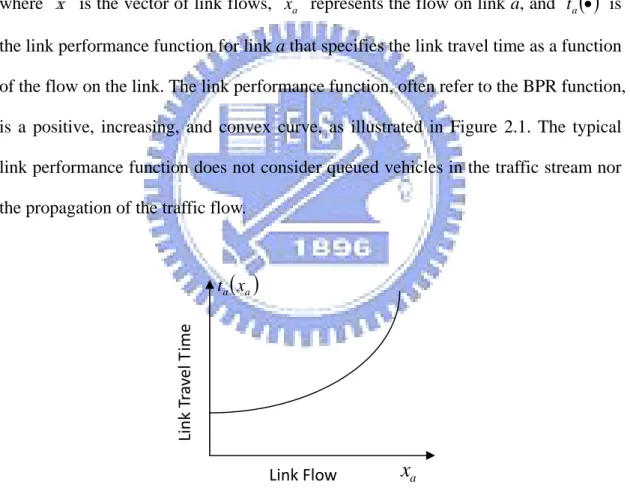
∀ = r s k rs k a rs k a f a x δ _, (2.2d)

where x is the vector of link flows, x_a represents the flow on link a, and t_a

( )

• is the link performance function for link a that specifies the link travel time as a function of the flow on the link. The link performance function, often refer to the BPR function, is a positive, increasing, and convex curve, as illustrated in Figure 2.1. The typical link performance function does not consider queued vehicles in the traffic stream nor the propagation of the traffic flow.

Figure 2.1 Typical Link Performance Function ta(xa)

The O-D demand between origin r and destination s is denoted by q_rs and the flow for O-D pair r-s assigned to path k is represented by f_krs. The static link-path incidence matrix relating path flows to link flows (equation 2.2d) are defined using

Link Flow Link Tr av e l Ti m e

( )

a a x t a

x

(18)

link-path incidence variable δ_a,rs_k as follows: ⎩ ⎨ ⎧ − = otherwise , 0 pair D -O between path on is link if , 1 , s r k a rs k a δ (2.2e)

The objective function Z(x), which is the sum over all arcs of the integrals of the link performance functions, does not have an intuitive economic or behavioral interpretation and is viewed strictly as a mathematical construct to solve equilibrium problems. Equation 2.2b indicates the set of flow conservation constraint which imply that all O-D demand have to be assigned to the network. The non-negativity conditions (equation 2.2c) ensure the solution of the program is physically meaningful. The network structure enters the formulation through the link-path incidence relationship (equation 2.2d) that relates the link-based objective function to the path-based constraint set.

Sheffi gives a comprehensive treatment of the static UE problem, addressing the conceptual, mathematical, algorithmic and computational aspects of the problem (Sheffi, 1985). A more difficult problem with asymmetric link interactions is addressed by Dafermos, and Fisk and Boyce by using variational inequality (VI) techniques (Dafermos, 1980, 1982; Fisk and Boyce, 1983). Nagurney, Mahmassani and Mouskos, and Patricksson address computational issues related to the VI problem (Nagurney, 1984,1986; Mahmassani and Mouskos, 1988, 1989).

System Optimal Concept

The other major class of assignment is system optimal (SO) formulation. The SO seeks a flow pattern that achieves some system-wide objectives. The static SO

(19)

10

assignment problem can be formulated as follows:

∑

= a a a at x x Z( ) ( ) min x (2.3a) subject to s r q f k rs rs k = ∀ ,

∑

(2.3b) s r k f_krs ≥0 ∀ , , (2.3c)

∑∑∑

∀ = r s k rs k a rs k a f a x δ _, (2.3d)

The objective function is the only difference from UE formulation with the interpretation of total system travel cost. The SO flow pattern does not always represent an equilibrium solution, as individual travelers may reduce their travel time by switching their routes. Hence, the SO flow pattern is not expected to hold without some control strategy such as road pricing or restriction. Consequently, the SO flow pattern is not an appropriate descriptive model of actual user behavior. It can be treated as a performance index of the network. The solution procedures for SO are identical to those of UE except that they differ in the specification of link cost functions (average cost function in UE; marginal cost function in SO).

Ben-Akiva enumerates the shortcomings of using static models in modeling congestions (Ben-Akiva, 1985). The static assignment has a major shortcoming of inadequately link congestion model. As discussed earlier in the thesis, the congestion is presented by a link performance function which gives the average trip time as a function of the average link flow. The average link flow can even exceed the actual capacity of the road section which is unrealistic for the control purpose. Another major problem lies on the description of traffic propagation. The static volume-delay

(20)

curve cannot describe the propagation of traffic flow, especially in high flow levels. Thereby, static assignment models are inappropriate for real-time traffic control application, especially for congested networks.

2.2 Dynamic Trip Assignment Models

Dynamic network assignment is under intensive research, for both user equilibrium and system optimal problems. One common feature of these researches is that they differ from the standard static assignment assumptions to deal with time-varying flows. Another feature shared by these researches is that none presently provides a universal solution for general networks.

The first attempt to formulate the DTA problem as a mathematical program is introduced by Merchant and Nemhauser (1978a, 1978b). The model (referred to as the M-N model) is limited to the fixed-demand, single-destination, deterministic, system optimal scenario. A link exit function is utilized to propagate traffic and a static link performance function is introduced to present the travel cost as a function of link flow. It results a flow-based, discrete time, non-convex non-linear programming formulation. The global solution can be derived by solving a piecewise linear version of the model.

System Optimal Concept

Carey (1987) reformulates the M-N model as a convex nonlinear program by the manipulation of exit function, which gives mathematical advantage over the original M-N model. The formulation differs from M-N model mainly in the consideration of multiple destinations, and the exit function g_a(•).

(21)

12

( )

∑∑

= t a t a t a t a x x h Z( ) min x (2.4a) subject to

( )

x b a t g_a _at ≥ _at ∀ , (2.4b) t a d x x b_at = t_a− t_a+1+ _at ∀ , (2.4c)

( )

, ( ) , ,t b B k c C k a b F d c t c t k b t b = +

∑

∀ ∈ ∈

∑

(2.4d) a E x_a0 = _a ∀ (2.4e) t a x d b_at, _at, _at ≥0 ∀ , (2.4f)

where x represents the number of vehicles on link a at the beginning of interval t. t_a

( )

t a t a x

h represents the travel cost incurred by the volume x and assumed to be _at

continuous, convex, nondecreasing and nonnegative. The variable b and _at d _at

denote the number of vehicle exiting and entering link a in interval t, respectively.

t k

F is referred to the exogenous demand at node k in period t. E_a is the initial volume on arc a. B

( )

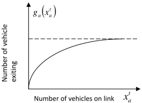
k and C(k) respectively represent the set of links incident from and to node k. g_a(•) the exit function define the maximum number of vehicles that can exit from link a and is a function of traffic conditions on the link; it is assumed to be a continuous, non-negative, non-decreasing, and concave function. Figure 2.2 illustrates a possible shape of such link exit function.

(22)

Figure 2.2 A possible shape of link exit function

Although after the manipulation of exit function, the formulation is convex, but it remains problematic by the non-convexity issues arising from first-in first-out (FIFO) requirement. The FIFO violation implies some traffic physically jumps over another to reduce system cost which is inconsistent with traffic realism. The FIFO requirement is easily satisfied in single destination formulation. While facing general networks, the FIFO requirement would introduce additional constraints that yield a non-convex constraint set and increasing the computational burden severely (Carey, 1992). As SO flow patterns, it may often be advantageous to favor certain traffic movement over others to minimize system-wide travel cost. For example, traffic at minor approach of an intersection may be holding back in favor of the major approach. That means vehicles may be artificially delayed for a time that might be considered as

unfair or unreasonable; and the flow pattern may not be acceptable for real-world

operation. Ziliaskopoulos introduces a linear programming formulation for the single destination system optimal DTA problem based on the cell transmission model (Ziliaskopoulos, 2000; Daganzo, 1994). This model circumvents the need for link performance function as the flow propagates according to the cell transmission model, hence is more sensitive to traffic realities.

t a

x

Number of vehicles on link Number of v ehicle ex iting

( )

t a a x g

(23)

14 User Equilibrium Concept

The user equilibrium formulation is generalized from the Wardrop condition for the static problem; it becomes the equilibration of the experienced path travel times of users. Janson represents one of the earliest attempts at modeling the UE dynamic traffic assignment problem as a mathematical program (Janson, 1991). The link-based UE model formulated as a mathematical program as follows:

( )

=

_∑∑∫

( )

t a x t a t a d Z 0 min x λ ω ω (2.5) subject to Equation (2.4b) – (2.4f)

The λt_a represents the cost of traveling link a at the beginning of interval t when there exist x vehicles on the link. _at

Birge and Ho extend the M-N model to the stochastic case by relaxing the assumption that O-D demands are known for the entire planning horizon (Birge and Ho, 1993). It assumes a finite number of scenarios, defined as a possible combination of past O-D demands in every time interval, while assignment decisions are independent of future O-D demands.

Another approach is modeling dynamic traffic assignment problem in a continuous manner. The O-D demands are assumed to be known continuous functions of time; link flows are treated as continuous functions of time. Constraints of optimal control formulations are analogous to those of the mathematical programming formulations, but they are defined in a continuous-time manner. Friesz et al. discuss link-based optimal control formulation for both SO and UE objectives for the single

(24)

destination case (Friesz, Luque, Tobin, and Wie, 1989). The model assumes that changes from one system state to another may occur concurrently as the network conditions change; that implies the routing decision are made based on current network conditions, and can be continuously modified as conditions change. The SO model is represented as follows:

( )

=

_∑∫

( )

a T a a x dt C Z 0 min x (2.6a) subject to

( )

_{( )}

_[

_{( )}

_]

_{[ ]}

T t A a t x g t u x dt t dx a a a a a , 0 , ∈ ∈ ∀ − = ≡ & (2.6b)

( )

( )u t ( )g

[

x

( )

t

]

k M t

[ ]

T t S k B a a a k A a a k =

∑

−

∑

∀ ∈ , ∈ 0, ∈ ∈ (2.6c)

( )

x a A x_a 0 = _a0 ≥0 ∀ ∈ (2.6d)

( )

t a At

[ ]

T u_a ≥0 ∀ ∈ , ∈ 0, (2.6e)

Equation 2.5b describe the rate of change of traffic volume with respect to time for link a will be considered as the difference of the flow entering link a, u_a

( )

t , and the flow exiting link a, ga

[

xa

( )

t

]

. In equation 2.6c, Sk

( )

t represents the traffic flow

generated at node k, which is assumed to be a nonnegative and continuous function of time. A

( )

k and B(k) respectively represent the set of links incident to and from node k. The nonnegative constraints of both traffic volume on the link and traffic volume entering the link are indicated in equation (2.6d) and (2.6e). As for the UE case, the objective function is illustrate as follows,

(25)

16

( )

=

_{∑∫ ∫}

( ) ( )

′ a T x a a a a a a dt d g c Z 0 0 min x ω ω ω (2.7) subject to equation (2.6b)-(2.6e).

The model proves that at the optimal solution, the instantaneous flow marginal costs on the used paths for an O-D pair are identical and less than or equal to the ones on the unused paths. As for the UE case, the model is in the form of equilibration of instantaneous user path costs.

Ran et al. use the optimal control approach to obtain a convex model for the instantaneous UE dynamic traffic assignment problem by defining link inflows and outflows to be control variables (Ran, Boyce, and LeBlanc, 1993) They recognize the inability of the usual cost functions to account for dynamic queuing and congestion costs, and propose splitting the link travel cost into moving and queuing parts. Boyce et al. proposed a methodology to solve the above model using Frank-Wolfe algorithm, but no implementations are illustrated (Boyce, Ran, and LeBlanc, 1995).

Because of the limitations of obtaining analytic mathematical properties, researchers focused on analytical DTA models have gradually migrated toward the variational inequality (VI) formulations. Variational inequality provides a general formulation platform for several different problems. Variational inequality approach is first introduced to the static traffic equilibrium by Dafermos (1980). Friesz et al. introduce the VI formulation into network design problem and suggest a sensitivity analysis based heuristic algorithm (Friesz, Tobin, Cho, Mehta, 1990; Friesz, Cho, Mehta, Tobin, Anandalingam, 1992). Friesz et al. is the first to show there is a variational inequality formulation of dynamic user equilibrium with simultaneous route choice and departure time decisions (Friesz, Bernstein, Smith, Tobin, Wie,

(26)

1993). Wie et al. formulate the dynamic network user equilibrium problem as a variational inequality problem in discrete time in terms of unit path cost functions (Wie, Tobin, Friesz, Bernstein, 1995). They also demonstrate that, assuming certain regularity conditions hold, discrete time dynamic network user equilibrium is

guaranteed to exist. They define the time varying flow pattern h* and associated

minimum cost μ* is a discrete time dynamic network user equilibrium if the

following conditions are satisfied:

( ) ( )

[

c t h h

]

p P i I j J t T t h_p*( ) _p , * −μ_ij * =0 ∀ ∈ _ij, ∈ , ∈ , =0,1,..., (2.8a)

( ) ( )

t h h p P i I j J t T c_p , * −μ_ij * ≥0 ∀ ∈ _ij, ∈ , ∈ , =0,1,..., (2.8b) J j I i Q t h ij P p ij T t p = ∀ ∈ ∈

∑∑

∈ = , ) ( 0 * (2.8c) T t J j I i P p t h*_p( )≥0 ∀ ∈ _ij, ∈ , ∈ , =0,1,..., (2.8d)

In equation 2.8, i and j are the origin and the destination node respectively. P _ij

denotes the set of all possible paths between origin i and destination j. )h_p(t is the number of vehicles entering the first link on path p in period t, and

[

h t p P t T

]

h= _p( ): ∈ , =0,1,..., . c_p

( )

t,h is the nonnegative unit travel cost incurred by travelers departing their origin in period t and choosing path p to their destination.

( )

h =

[

μ_ij

( )

h :i∈I,j∈J

]

μ is the vector of minimum unit travel costs. Q is the total _ij

fixed O-D demand between i and j during time interval 0≤t≤T. Since a complete

path enumeration is required, an efficient method to identify a possible path set should be introduced to relief the computation burden.

Ran and Boyce propose a link-based discretized VI formulation SO DTA model with fixed departure time (Ran and Boyce, 1996). They equilibrate the experience

(27)

18

travel time, the same as Friesz (1993). A queuing delay component is introduced in the model, but the capacity and oversaturation constraints increase the computation complexity significantly. Chen and Hsueh propose a link-based VI formulation UE DTA model and a nested diagonalization solution algorithm (Chen and Hsueh, 1998). The constraint set of the model is nonlinear and nonconvex, and multiple local solutions might exist. The variational inequality approach gives greater analytical flexibility and convenience than other analytical approaches. Although it brings mathematical advantages, the variational inequality approach is much more computationally intensive, especially facing the complete path enumeration for path-based formulation.

Simulation based models are mostly based on the mathematical programming models, but the critical constraints that describe the traffic flow propagation (i.e. flow conservation, vehicular movement) are addressed through simulation instead of analytical representation. With the traffic simulation, these models can address the traffic flow more realistic. However, the theoretical insights cannot derive analytically, which is the key issue of simulation-based models. A deterministic DTA model, with both SO and UE solutions, is proposed by Mahmassani and Peeta (1993). A meso-scopic traffic simulator is used as part of an iterative algorithm, with complete priori information of O-D demands for the entire planning horizon. Ghali and Smith propose a deterministic SO DTA model with congestion arises exclusively at specified bottlenecks modeled as deterministic queues (Ghali and Smith, 1995). Simulation based models can describe the traffic flow more realistic, which is troublesome in analytical formulations. However, the limitation lies on the inability to derive the associated mathematical properties.

(28)

assignment matrix between time-dependent O-D flows and link volumes both in off-line and real-time application (Ashok and Ben-Akiva, 2002). Ben-Akiva et al. propose DynaMIT, a meso-scopic simulator, as a dynamic traffic assignment system to estimate and predict current and future traffic conditions (Ben-Akive, Koutsopoulos, Mishalani, Yang, 1997). The model considers both historical information and drivers’ response to information, supply and demand simulators work together to generate UE route guidance. Nie and Zhang proposed a relaxation approach for estimating static O-D matrix that minimizes a distance metric between measured and estimated traffic condition while the condition satisfies user equilibrium (Nie and Zhang 2008).

2.3 Summary and Discussion

To design and manage a transportation system, there is a need for efficient analyzing tool to describe the usage of the system. The traditional static method, four-stage planning process, includes trip generation, trip distribution, modal split, and trip assignment. Traditional sequential four-stage method is not suitable in the operation perspective. Since the travel costs used in the trip distribution stage are functions of the trip assignment outcomes; that is, the stages have to be repeated. From the literature review, estimate the network flows directly from time-series of link flows seems to be a reasonable candidate for real-time traffic operation aspect.

This chapter has reviewed several topics relevant to the trip assignment problems. Most existing research works assumed the existence of user-equilibrium or system-optimal conditions. However, the existence of equilibrium states in real traffic networks is questionable; an alternative approach to relax the assumption of user-equilibrium or system optimal might worth be established.

(29)

20

Chapter 3 A Path-base Assignment Model with Time-invariant

Coefficient Dynamic System

In this chapter, some essential concepts of the path-base assignment model with time-invariant coefficient dynamic systems are discussed. Begin with the brief introduction to dynamic system models, the model assumption and notation is addressed in section 3.1. A state space approach that modeled the path estimation is illustrated in section 3.2. Link dynamics that describe the propagation of traffic flows is introduced, in section 3.3, to modify the proposed model.

3.1 Assumption and Notation

Existing research works on traffic assignment usually assume the existence of user equilibrium status or pursuit some system optimal situation. However, it is questionable whether such equilibrium state really exists or not. In this study, we relax such assumption by some statistical approaches.

The basic assumption in this research is the existence of unknown relationship between consecutive path-flows; the assumption is similar to that of Okutani. While Okutani assumed a time invariant relation between time-series O-D flow exists; and this relationship can be estimated by some prior information. In this study, we do not estimate the relationship by prior information; the relationship is estimated simultaneously with path flows.

(30)

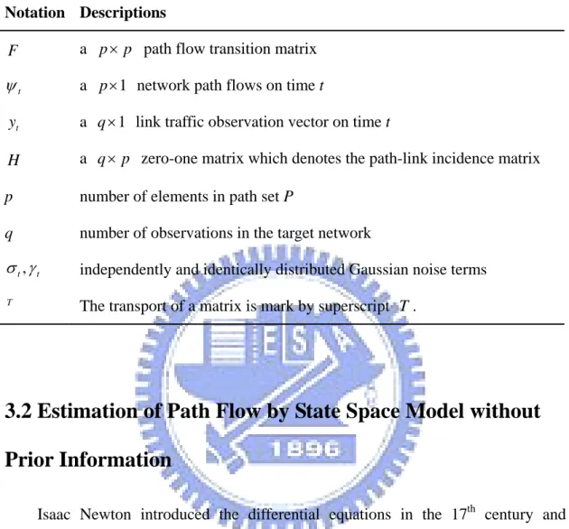
Table 3.1 Notations of Time-invariant State Space Model

3.2 Estimation of Path Flow by State Space Model without

Prior Information

Isaac Newton introduced the differential equations in the 17th century and

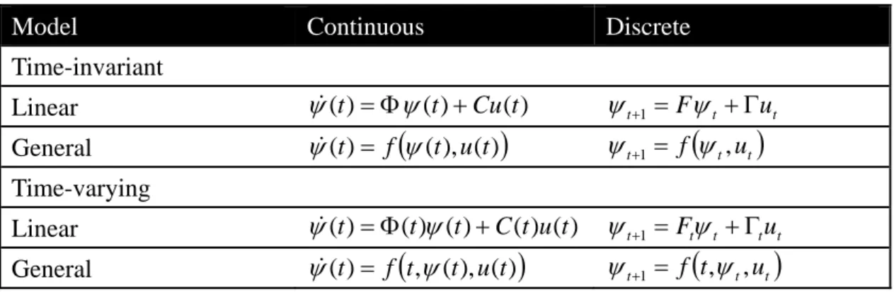
provided mathematical models for many dynamic systems. Given a finite number of initial conditions, one can uniquely determine the system status for all time. The finite dimensional representation of a problem is the basic idea for the state-space approach to the representation of dynamic systems. The dependent variables of the equations are the state variable of the dynamic systems. The principal dynamic system models are listed in Table 3.2 below.

Notation Descriptions

F a p× path flow transition matrix p

t

ψ a p×1 network path flows on time t

t

y a 1q× link traffic observation vector on time t

H a q× zero-one matrix which denotes the path-link incidence matrix p

p number of elements in path set P

q number of observations in the target network

t t γ

σ , independently and identically distributed Gaussian noise terms

(31)

22

Table 3.2 Principal dynamic system models

Reference: [Grewal & Andrews, 1993]

We focused on the discrete dynamic systems in this dissertation. In the dynamic

model, F is a n×n dynamic coefficient matrix. The matrix

[

]

T

n t ψ1(t) ψ2(t) ψ3(t) ψ (t)

ψ = _L is called the state vector, where ψn(t)

denotes the nth state variable in time t. The n-dimensional domain of the state vector is called the state space of the dynamic system. The state variables are related to the system outputs by a system of linear equations that can be represented in vector form, as follows. t t t H y = ψ +γ where

[

]

T l t y t y t y t y t y = ₁( ) ₂( ) ₃( ) _L ( ) ⎥ ⎥ ⎥ ⎥ ⎥ ⎥ ⎦ ⎤ ⎢ ⎢ ⎢ ⎢ ⎢ ⎢ ⎣ ⎡ = n l l l l n n n h h h h h h h h h h h h h h h h H L M O M M M L L L 3 2 1 3 33 32 31 2 23 22 21 1 13 12 11

The y_t is a l-vector called the measurement vector (also called observation vector)

Model Continuous Discrete

Time-invariant Linear ψ&(t)=Φψ(t)+Cu(t) ψ_t₊₁ =Fψ_t +Γu_t General ψ&(t)= f

(

ψ(t),u(t)

)

ψt+1 = f

(

ψt,ut

)

Time-varying Linear ψ&(t)=Φ(t)ψ(t)+C(t)u(t) ψt+1 =Ftψt +Γtut General ψ&(t)= f

(

t,ψ(t),u(t)

)

ψt+1 = f

(

t,ψt,ut

)

(32)

of the system. The matrix His a measurement sensitivity matrix with measurement sensitivities h measures the scale of _l_n th

l output to n state variable. th

Real world problems tend to have some kind of unpredictability in behaviors, due to some unknown exogenous inputs. Furthermore, output-measuring process with physical sensors will always introduce some amount of sensor noise, which will cause errors in the estimation process. While facing real world problems, using a statistical approach that taking uncertainties into account instead of deterministic would be a better approach. These dynamic systems with uncertainties are characterized by statistical parameters such as means, correlations, and covariances.

3.2.1 Modeling

In this section, only the most basic modeling is introduced. The transition matrix that describe the relationship among path-flows in different time period is assumed to be fixed. The link travel time, which is an important issue, is not considered. Although the above strict assumption are made in this section, but they will be relaxed in the following section.

State space model is introduced to estimate path flows from link traffic counts. The state space model is coupled with two parts: transition equations and observation equations. First, the state equation which assumed that the path flows at time t+1

can be related to the path flows at time t by the following autoregressive form,

n t

F _t _t

t = ψ −1+σ , =1,2,3,...,

ψ (3.1)

where ψ_t is the state vector which is unobservable, F is a random transition

(33)

24

p

N denotes the p-dimensional normal distribution, Σ is the corresponding

covariance matrix. ψ , the p×1 state vector, is defined to be the path flows

belonging to O-D pairs.

Next, the observation equation,

n t

H

y_t = ψ_t +γ_t, =1,2,3,... (3.2)

where y is the _t q×1 observation vector which means there are q detectors on the

network. The number of paths is denoted by p . H is a q× zero-one matrix, p

which denotes the path-observation incidence matrix. The path-observation is pre-determined by generating possible path set and given travel time on each link. γ_t is also a noise term that γ_t ~ N_q

( )

0,Γ . Both ψ and F are unobservable, thus

Kalman filter is not suitable to directly estimate and forecast the state vector. Hence, Gibbs sampler is used to tackle the problem of simultaneous estimation of F and

ψ by available information.

There are two major elements to be incorporated in the solution method, 1) filtering states by observations, and 2) sampling scheme of transition matrix, F , and

state vector, ψ . Since the observations,y , are not used in the conditional distribution, _t

the Kalman filter and the Gibbs sampler must be combined. After the estimation of state vector, O-D flows can be calculated by the summation of path flows.

3.2.2 Kalman Filter

Kalman filter is an estimator for the linear-quadratic-Gaussian problem, which estimates the instantaneous state of a linear dynamic system perturbed by Gaussian white noise. It utilizes measurements, corrupted by Gaussian white noise, linearly

(34)

related to the state and gives a statistically optimal estimator with respect to quadratic function of estimation error. The Kalman filter does not only provide a means for inferring missing information from indirect and noisy measurements, but also used for predicting the likely future trends of dynamic systems. The structure of the filter can be derived in a Bayesian framework as follows.

The first stage (i.e. t =1), there’s no observation exists, thus the state vector ψ₀ must be generated by a prior distribution thatψ₀ ~ N_p(μ₀,V₀), where μ₀ is the mean and V is the covariance matrix. By using equation (3.1), the distribution for the state ₀

vector in the first stage will be normal with parameters

[

t |yt−1

]

= t|t−1 =F t−1 Eψ μ μ (3.3)

[

₋

]

= ₋ = ₋ T +Σ t t t t t y V FV F Varψ | 1 | 1 1 (3.4)

where μ denotes the expect value of _t_t₋₁ ψt and Vt|t−1 denotes the variance of ψt

when y_t₋₁ is observed. By the above information, the forecast observation would be normal distribution with parameters

[

y_t |y_t₋₁

]

= yˆ_t =H _t_|_t₋₁ E μ (3.5)

[

₋

]

= = ₋ T +Γ t t t t t y M HV H y Var | ₁ _| ₁ (3.6)

The above equation (3.3)-(3.6) holds for any t.

As the new observation y_t become available, the parameter vector would be updated according to Baye’s rule,

(

t |yt

)

∝ p

(

yt | t

) (

p t |yt−1

)

(35)

26

By using Bayes’ rule and standard Bayesian theory, the posterior distribution will be normal with parameters

(

| 1

)

1 1 | 1 | | − − − − + − = t t tt T t t t t t t μ V H M y Hμ μ (3.7) 1 | 1 1 | 1 | | − − − − − = T _t _t_t t t t t t t V V H M HV V (3.8)

The algorithm of Kalman filter is illustrated as follows,

Algorithm Kalman Filter

Input:μ₀,V₀, y_t:=observationsequence

Output: Filtered μ and V Begin

FOR each time step of the observation sequence

Generate prediction of the new observation by

1 ˆ_t = H⋅F⋅ _t₋ y μ

(

⋅ ⋅ +Σ

)

+Γ = ₋ T T t t t H F V F H M | 1

Update the parameter by

(

| 1

)

1 1 | 1 | | − − − − + − = T _t _t _t_t t t t t t t μ V H M y Hμ μ 1 | 1 1 | 1 | | − − − − − = t tt T t t t t t t V V H M HV V END FOR END

(36)

3.2.3 Gibbs Sampler

Gibbs sampler is a technique for generating random variables from a distribution indirectly, without having to calculate the density. In this paper, we make the following assumptions, (i) The initial ψ₀ ~ N

(

μ₀,V₀

)

, (ii) The covariance matrix Σ and Γ are known, and (iii) Given F, the distribution ψ_t is Gaussian.

The state equation can be written

n t FT _tT T t T t =ψ −1 +σ , =1,2,3,L, ψ (3.9) that is ⎥ ⎥ ⎥ ⎦ ⎤ ⎢ ⎢ ⎢ ⎣ ⎡ + ⎥ ⎥ ⎥ ⎦ ⎤ ⎢ ⎢ ⎢ ⎣ ⎡ = ⎥ ⎥ ⎥ ⎦ ⎤ ⎢ ⎢ ⎢ ⎣ ⎡ − T n T T T n T T n T F σ σ ψ ψ ψ ψ M M M 1 1 0 1

The following notation is used for simplification.

⎥ ⎥ ⎥ ⎦ ⎤ ⎢ ⎢ ⎢ ⎣ ⎡ = T n T n ψ ψ M 1 ψ , ⎥ ⎥ ⎥ ⎦ ⎤ ⎢ ⎢ ⎢ ⎣ ⎡ = − − T n T n 1 0 1 ψ ψ M ψ , ⎥ ⎥ ⎥ ⎦ ⎤ ⎢ ⎢ ⎢ ⎣ ⎡ = T n T n σ σ M 1 σ ,

[

pT

]

T i T T F F F F = 1 _L _L

where F denotes the _iT th

i column vector of T

F . Then the equation (3.9) can be

re-written as n T n n ψ F σ ψ = ₋₁ +

Consider the element of S, the p× covariance matrix being used to estimate the p

variance-covariance matrix of F ,

( )

{

(

T

)

}

j T i ij T F F S F S = ,

(37)

28

where S denotes the _ij (i,j) element of the matrix. S can be calculated by the _ij

following equation.

(

)

(

)

(

)(

) (

)

(

T

)

j T j T n n T i T i T j T n T j n T i T n T i n T j T n T j n T T i T n T i n ij F F F F F F F F S ˆ ˆ ˆ ˆ ˆ 1 1 1 ) ( 1 ) ( 1 ) ( 1 ) ( − − + − − = − − = − − − − − − ψ ψ ψ ψ ψ ψ ψ ψ ψ ψ (3.10)

where Fˆ_iT =

(

ψ_n₋₁ψ_nT₋₁

)

−1ψ_n₋₁ψ_nT₍_i₎ is the least square estimate of F , and _iT ψ_n_(i₎ is the

th

i column vector of ψ_n. Consequently,

( )

(

)

T

(

T T

)

n n T T T T F F F F A F S = + − ˆ ψ ₋₁ψ ₋₁ − ˆ (3.11)

where A is a p× matrix. p A=

{ }

a_ij , where a is the _ij (i,j)elements of A, with

(

_nT₍_i₎ _nT₁ ˆ_iT

) (

T _nT₍_j₎ _nT₁ ˆ_jT

)

`

ij F F

a =ψ −ψ ₋ ψ −ψ ₋ . (3.12)

That means A is proportional to the sample covariance matrix. From the general result in the Gaussian model, the posterior distribution of F is then T

(

) ( )

(

)

(

)

2 1 1 2 ˆ ˆ , | n T T T n n T T T T n T T F F F F A F F S F p − − − − − − + = ∞ < < ∞ − ∝ ψ ψ ψ (3.13)

The distribution in equation (3.13) is a matrix-variate generalization of the

t-distribution. The following sampler for generating F and T ψ is then proposed. The sampling scheme generate from the conditional distributions

a. ψ_t|F,ψ_t₋₁,Σ~N

(

Fψ_t₋₁,Σ

)

b. FT|ψ,Σ~

[

k

(

n,p,p

)

]

−1A(n−p)/2ψ_n₋₁ψ_nT₋₁ p/2 A+Fψ_n₋₁ψT_n₋₁FT −n/2

The above sampling scheme would be the key component of the Gibbs sampler. The Gibbs sampler is a Markovian updating scheme that proceeds as follows. Given

(38)

an arbitrary starting set of values {Z₁(0),Z₂(0),Z₃(0),...,Z_k(0)}, and then draw ] ,... , [ ~ ₁ ₂(0) ₃(0) (0) ) 1 ( 1 Z Z Z Zk Z , ] ,... , [ ~ ₂ ₁(0) ₃(0) (0) ) 1 ( 2 Z Z Z Zk Z , ] ,... , [ ~ ₃ ₁(0) ₂(0) (0) ) 1 ( 3 Z Z Z Zk Z , … ] ,... , [ ~ ₁(0) ₂(0) (0)₁ ) 1 ( − k k k Z Z Z Z Z .

Each variable is visited in the natural order and a cycle requires k random variate generations. After i iterations we have ( , , (),..., ())

3 ) ( 2 ) ( 1 i k i i i Z Z Z

Z . Under mild conditions,

the following results hold (Geman and Geman, 1998)

Result 1: Convergence

As the iteration continue, (Z₁(i),Z₂(i),Z₃(i),...,Z_k(i))→

[

Z₁,Z₂,Z₃,...,Z_k

]

. Hence, for each sequence s, ]Z_s(i) →[Z_s as i→∞.

Result 2: Rate

Using the sup norm, the joint density of (Z₁(i),Z₂(i),Z₃(i),...,Z_k(i)) converges to the true density at a geometric rate, under visiting in the natural order.

Result 3: Ergodic theorem

For any measurable function T of Z₁,Z₂,Z₃,...,Z_k whose expectation exists,

(

)

(

k

)

i l l k l l l i _i T(Z ,Z ,Z ,...,Z ) ET Z ,Z ,Z ,...Z 1 lim ₁ ₂ ₃ 1 ) ( ) ( 3 ) ( 2 ) ( 1 →

∑

= ∞ → .

Then for every function T on the possible configurations of the system and for every starting configuration holds with probability one.

(39)

30

Analytical convergence rates for Gibbs sampler applied to state space models are further discussed by Pitt and Schephard in 1996 and Robert (Pitt and Schephard, 1996; Robert, 1998)

As Gibbs sampling through m replications of the aforementioned i iterations produces i independent and identically distributed k tuples Z₁(i_j),Z₂(i_j),Z₃(i_j),...,Z_kj(i),

m

j=1,2,3,..., , which the proposed density estimate for

[ ]

Z having form _s

[ ]

=

_∑

m₌

[

≠

]

j j r s s Z Z r s m Z 1 ) ( , 1 ˆ _.

The above Gibbs sampling scheme on a random transition matrix and state vector forms the center part of the algorithm. In the process of generate state vectors, Kalman filtering mechanism is added. While a simple monitoring of the chain (Zs) can

only expose strong non-stationarities, it is more relevant to consider the cumulated sums, since they need to stabilize for convergence to be achieved. The convergence control of Gibbs sampler is discussed in chapter 5.

Algorithm Gibbs Sampler

Input: H := path−observationincidencematrix, y_t :=observationsequence

Output: ψˆ,Fˆ Begin Initialize p I F(0):= , Σ :=I_p, Γ :=I_p

{ }

φ = store ψ , F_store =

{ }

φ SET GibbsCount (g) to 0 WHILE not Converge

(40)

Generate ψ(g) ~N

(

μ,V

)

Append ψ( g)

to ψstore

CALL Kalman Filter with μ,V , and observation sequence

Generate FT( g) by

{ }

( ) ) ( g ij g a A = , a_ij =

(

ψ_nT₍_i(₎g)−ψ_nT₋(₁g)Fˆ_iT(g)

) (

Tψ_nT₍(_jg₎)−ψ_nT₋(₁g)Fˆ_jT(g)

)

Generate w Wishart

(

XT g n p

)

n g n− − , − ~ (1) ) ( 1 ψ Generate Z =

(

z₁T,zT₂,z₃T,...,zT_p

)

, ~ _p

(

0, (g)

)

iid k N A z COMPUTE F w Z T g T 1 2 1 ) ( − ⎟ ⎟ ⎠ ⎞ ⎜ ⎜ ⎝ ⎛ ⎟⎟ ⎠ ⎞ ⎜⎜ ⎝ ⎛ = APPEND T( g) F to Fstore INCREMENT GibbsCount END WHILE

READ last k items from ψ_store and put in ψ_n

COMPUTE =

∑

_n

k ψ

ψˆ 1

READ last k items from F_store and put in F _n

COMPUTE =

∑

F_n

k Fˆ 1

END

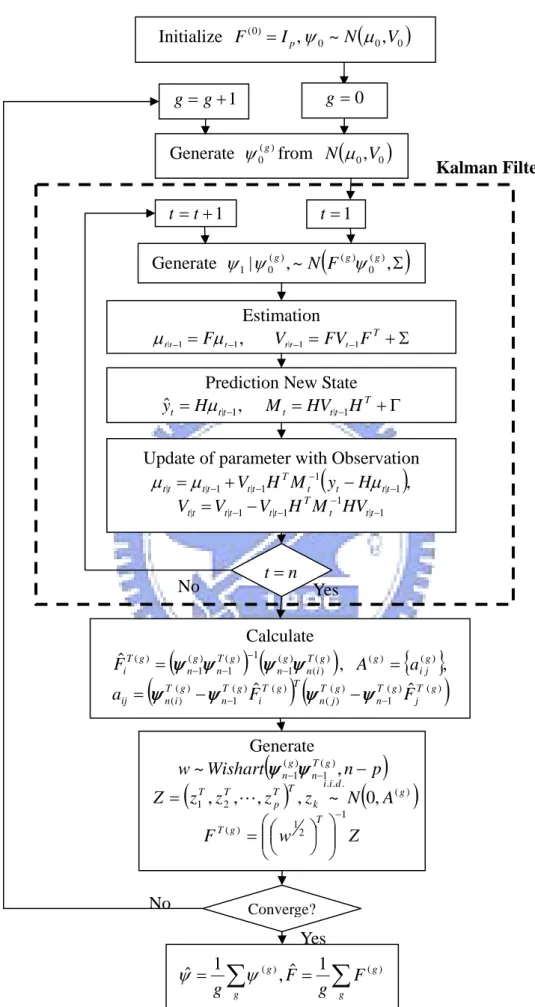
3.2.4 Solution Framework

In this section, the solution framework of applying Gibbs sampler and Kalman filter to the state space model is illustrated. The solution framework that combines the algorithm in both section 3.2.2 and 3.2.3 is demonstrated in figure 3.1. The solution

(41)

32

framework is an iterative estimation of state vectors and transition matrix; the iteration counts are denoted as g . It first filters the state vector by given transition

matrix, path-observation incidence matrix (some may refer as mapping matrix), and observation vector; and then turns to estimate the transition matrix by filtered state vector. During the Kalman filter stage of the framework, transition matrix and mapping matrix are fixed; while in the transition matrix estimating stage, the state vector is fixed. As the algorithm reach convergence, the transition matrix, Fˆ , and state vector, ψˆ, can be estimated.

After deriving transition matrix and state vector, the prediction of state vector can be represent as,

1 1

ˆ_t₊ =F⋅ψ_t+σ_t₊

ψ . (3.14)

And the estimation of ψˆ_t₊_h is

(

)

(

)

(

)

(

)

(

t t t h t h

)

t h h t h t h t h t h t h t F F F F F F F F + − + − + + + − + − + + − + + + + + + ⋅ ⋅ ⋅ ⋅ = + + ⋅ ⋅ = + ⋅ = σ σ σ σ ψ σ σ ψ σ ψ ψ 1 2 1 1 2 1 ˆ ˆ ˆ L L (3.15)

Since the expectation value of σ is zero. The estimate of ψˆ_t₊_h can be written as

t h h

t F ψ

(42)

Figure 3.1 The solution framework of state space model Initialize F(0) =I_p,ψ₀ ~N

(

μ₀,V₀

)

Generate 0( ) g ψ from N

(

μ0,V0

)

Generate | ,~

(

0( ),Σ

)

) ( ) ( 0 1 g g g F N ψ ψ ψ Estimation , 1 1 |t− = t− t Fμ μ V_t_|_t₋₁ =FV_t₋₁FT +Σ

Prediction New State , ˆ_t =H _t_|_t₋₁ y μ M_t =HV_t_|_t₋₁HT +Γ 1 + = t t

Update of parameter with Observation

(

_| ₁

)

, 1 1 | 1 | | − − − − + − = T _t _t _t_t t t t t t t μ V H M y Hμ μ 1 | 1 1 | 1 | | − − − − − = T _t _t_t t t t t t t V V H M HV V n t= No Calculate

(

) (

( )

)

) ( ) ( 1 1 ) ( 1 ) ( 1 ) ( ˆ T g i n g n g T n g n g T i F = ψ ₋ψ ₋ − ψ ₋ψ , ( )

{ }

i(gj) , g a A =

(

) (

( ) ( )

)

1 ) ( ) ( ) ( ) ( 1 ) ( ) ( ˆ ˆ g T j g T n g T j n T g T i g T n g T i n ij F F a = ψ −ψ ₋ ψ −ψ ₋ Generate

(

n p

)

Wishart w~ ψ_n(₋g₁)ψ_nT₋(₁g), −

(

)

.. .

(

( )

)

2 1 , , , , ~ 0, g d i i k T T p T T A N z z z z Z = _L Z w F T g T 1 2 1 ) ( − ⎟⎟ ⎠ ⎞ ⎜⎜ ⎝ ⎛ ⎟ ⎠ ⎞ ⎜ ⎝ ⎛ = Converge?

∑

= = g g g g F g F g ) ( ) ( _ˆ 1 , 1 ˆ ψ ψ No Kalman Filter 1 + = g g g =0 1 = t Yes Yes

(43)

34

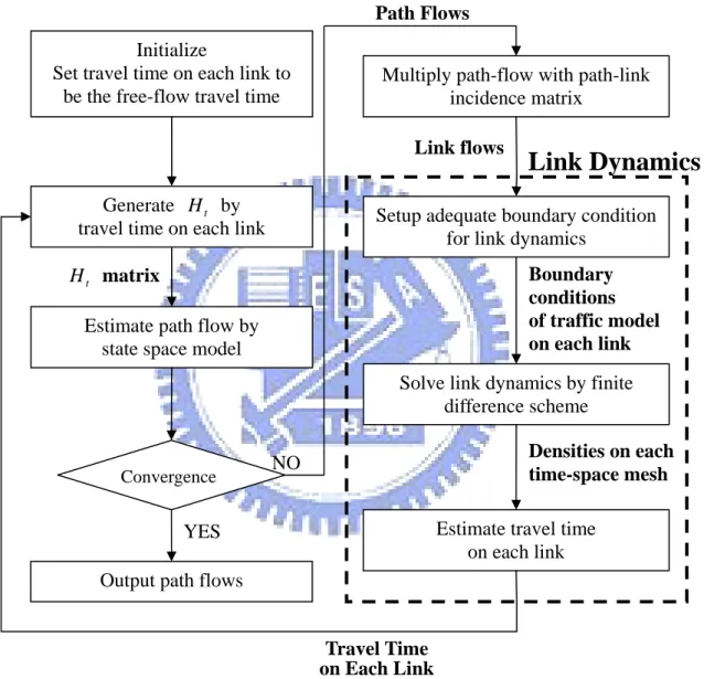
3.3 Estimation of Path Flow Considering Link Travel Time

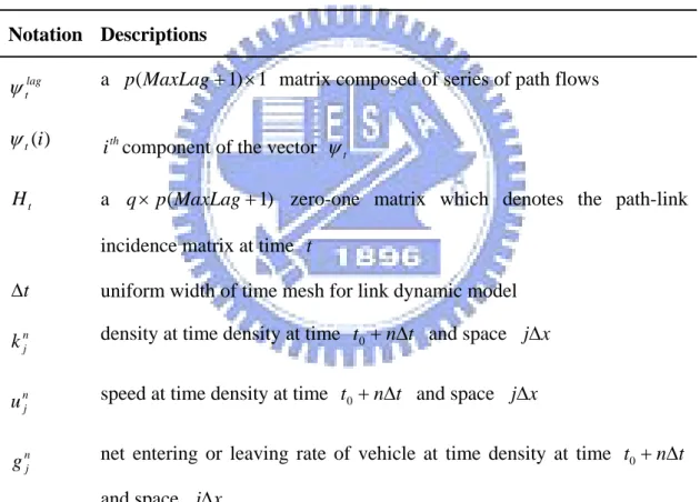
Travel time is an important issue while facing transportation problems. It is no exception in path flow estimation. We relax the assumption of zero travel time in this section. To describe the flow propagation from its origin to destination, travel time on each links should be considered. A macroscopic traffic continuum model, the PW model, is introduced to describe the link dynamics. Notations increased or changed in the section is shown in table 3.3.

Table 3.3 Notations of Time-invariant State Space Model considering Link Travel Time

3.3.1 Modeling

The model in this section had been modified from the previous section (section 3.2) to consider travel time effect. The state transition equation is the same as in

Notation Descriptions

lag t

ψ a 1p(MaxLag+1)× matrix composed of series of path flows )

(i

t

ψ th

i component of the vector ψ_t

t

H a )q× MaxLagp( +1 zero-one matrix which denotes the path-link

incidence matrix at time t

t

Δ uniform width of time mesh for link dynamic model

n j

k density at time density at time t0 +nΔt and space jΔ x

n j

u speed at time density at time t0 +nΔt and space jΔ x

n j

g net entering or leaving rate of vehicle at time density at time t0 +nΔt

(44)

previous section, but the observation equation had been modified as follows. n t F _t _t t = ψ −1+σ , =1,2,3,..., ψ (3.17) n t H y_t = _tψ_tlag +γ_t, =1,2,3,... (3.18)

The state variable,ψtlag , is modified here to take the travel time into account. It is a

1 ) 1 (MaxLag+ ×

p matrix composed of series of state vectors,

{

_T

}

T MaxLag t T t T t T t lag t = ψ ψ − ψ − ψ − ψ ₁ ₂ _L .

Let the element inψ_t, a p×1 vector, be represent as

1 ) ( ) 2 ( ) 1 ( × ⎥ ⎥ ⎥ ⎥ ⎦ ⎤ ⎢ ⎢ ⎢ ⎢ ⎣ ⎡ p t t t p ψ ψ ψ M . Then,

[

t t t

]

_p T t = ψ (1) ψ (2) ψ (p)1× ψ _L , and

[

][

]

{

[

][

]

}

T ₍ ₎ MaxLag p MaxLag t MaxLag t MaxLag t MaxLag t t t t t lag t p p p p 1 1 1 1 1 1 ) ( ) 1 ( ) ( ) 1 ( ) ( ) 1 ( ) ( ) 1 ( + × − − + − + − − − = ψ ψ ψ ψ ψ ψ ψ ψ ψ L L L L L .

The term MaxLag denotes the maximum time lag that path flow can be observed on observation sites at time t . The path-observation incidence matrix, H , is a zero-one _t

) 1

( +

× MaxLagp

q matrix at time t . If the path flow of a certain time can be

observed at detector q , then the corresponding element in H is one; else, it is zero. _t

The incidence matrix can be generated by the interaction with link dynamics that is described in the next section.

以貝氏方法構建與求解路徑基礎之時變交通指派模式

國

立

交

通

大

學

運 輸 科 技 與 管 理 學 系

博 士 論 文