參數空間法用於擾動控制系統之分析與設計

國

立

交

通

大

學

電機與控制工程學系

博 士 論 文

參數空間法用於擾動控制系統之分析與設計

Analysis and Design of Perturbed Control Systems Based on

Parameter Space Method

研 究 生：秦弘毅

指導教授：吳炳飛 博士

參數空間法用於擾動控制系統之分析與設計

Analysis and Design of Perturbed Control Systems Based on Parameter

Space Method

研 究 生：秦弘毅 Student：Hung-I Chin

指導教授：吳炳飛 博士 Advisor：Dr. Bing-Fei Wu

國 立 交 通 大 學

電 機 與 控 制 工 程 學 系

博 士 論 文

Submitted to Department of Electrical and Control Engineering College of Electrical Engineering and Computer Science

National Chiao Tung University In Partial Fulfillment of the Requirements

for the Degree of Doctor of Philosophy

in

Electrical and Control Engineering

June 2005

參數空間法用於擾動控制系統之分析與設計

研究生：秦弘毅 指導教授

吳炳飛 博士

國立交通大學電機與控制工程學系

摘

要

在實體系統中使用的模型通常是不準確的。在運作期間，系統中

的參數常隨著時間和環境的變化而改變，或者由於使用之模型為簡化

的模型，凡此種種原因皆可導致誤差的產生，所以針對特定準確的系

統而進行之分析及設計是不完全實用的。在實際控制系統設計及分析

時，穩健的系統穩定性，是重要的考慮因素。由於系統中非線性元件

的存在，另一個必須考慮的重要現象為極限環的產生，而通常這是設

計者不希望見到的，此類問題已經被許多的研究者討論過。對帶有非

線性性質的擾動系統而言，如果能夠事先預測其極限環的行為，對設

計者是極有助益的。利用描述函數法將非線性元件線性化，以預測其

極限環的發生，已成功的使用在許多的應用上。

本論文旨在針對具有擾動參數的控制系統，提出一完整且有效之

方法，利用參數空間法及穩定性的基本觀念，以分析其增益邊際和相

位邊際，並且設計控制器，調整控制器的係數，以達到系統頻域的規

格要求，例如增益邊際、相位邊際和敏感度。同時對有非線性元件的

系統，預測其極限環的發生。車輛模型被使用為模擬的例子。藉著求

解系統之特性方程式，在選定之系統參數平面或空間上，產生增益及

相位邊界曲線，以圖解方式決定控制器係數的合格區域，以使整個系

統之性能達到頻域規格的要求，以此法進行分析及設計。同樣的方法

也應用於模糊控制系統穩定度的分析。以上提出之方法更進一步延伸

至具有擾動參數的鎖相迴路系統的設計分析。部分系統參數在給定區

域擾動，於參數平面上，以圖形顯示待決之目標參數區域，選定該區

域範圍內之參數，使該鎖相迴路系統能達到規格之要求。本論文模擬

的結果已驗証了預期達成之目標。

Analysis and Design of Perturbed Control Systems Based on

Parameter Space Method

Student：Hung-I Chin Advisor：Dr. Bing-Fei Wu

Department of Electrical and Control Engineering

National Chiao Tung University

ABSTRACT

The models used are usually imprecise and the parameters of physical

systems vary with the operating conditions and time. Designing and

implementing a system for a fixed and exact control plant is not usually

practical in the natural environments. A inaccurate plant may result from a

simplified model and uncertainties in system parameters can always occur

in the physical world. Robustness stability is important in analysis and

design of practical control systems. Another important phenomena to be

considered is undesirable oscillations due to nonlinearities in a feedback

closed system and it has been studied by many researchers. It is very

instructive for the designer to predict the limit cycle behavior of a

perturbed control system with nonlinearities. The describing function

technique is mainly employed to predict the existence of constant

amplitude oscillations of closed nonlinear systems and has been

successfully used in many applications.

The main subject of this dissertation is to propose a novel method

based on parameter space method and robust stability criteria to predict

limit cycles occurred, analyze the system performances of gain margin and

phase margin (GM and PM), and design a desired controller by adjusting

the controller coefficients for perturbed control systems to meet specified

conditions including GM, PM and sensitivity in frequency domain. A

vehicle model is used as an example for simulation. With the help of gain

and phase boundary curves resulting from the roots of the characteristic

polynomial equation of closed control systems, a methodology is proposed

for portraying regions in a selected designed parameter plane so that the

performance of the whole system can meet the specified requirements with

perturbed parameters varying in given intervals. The same approach is

extended to analyze the robust stability for a fuzzy control system. This

dissertation also applies the above method on phase-locked loops (PLL)

design by frequency domain approach for a perturbed PLL system. The

desired system parameters of PLLs in the selected coordinate plane are

determined in graphical portrayals. Simulation results have demonstrated

and achieved the objectives as desired.

誌謝

這一路走來，有太多我需要感謝的人!

尤其是我的論文指導教授 吳炳飛老師。

在此我要由衷的向您和師母的關心表示十二萬分的謝意和敬意。

由於您的鼎力協助、指導研究，並給予不斷的鼓勵，尤其遭遇挫折的

時候，才使我越挫越能堅持。

特別感謝口試委員 鄧清政教授、張志永教授、林志民教授、鍾俊

業教授、黃英哲教授,在百忙之中，願意撥冗參與口試，不吝給予鞭策

和指導。

在研究過程中，彭昭暐博士經常給予協助和提供諸多建議，給予

研究上極大的助益，多年來彭博士及淑美賢伉儷所展現的友誼關懷，

尤其令我銘感五內，永誌難忘。

感謝 CSSP 實驗室的學弟妹們多年來提供的協助，您們的友情，給

了我一切。您們的勤奮和努力，使也我印象深刻，值得向年輕的各位

再學習，尤其是立山、世孟。

多年來，內人 素瑩體諒我就讀研究所博士班，課業繁重，協助我

照料家庭及子女，免除後顧之憂，使我能潛心向學，最值得我感謝。

希望在未來人生旅途上，能以實際行動，回報一二。也謝謝小兒 國鈞

及小女 瑋苓的加油、鼓勵，給予我無比的勇氣。

有所遺憾的是博士班就讀期間，父親、母親相繼辭世，使我未能

多盡人子孝道，回饋養育恩情，謹於此，表達對我的父親 秦瓊樹先生、

母親 秦黃含笑女士感恩及紀念之意。

「天行健，君子以自強不息」，人生就是不斷的學習過程。雖已

年過半百，仍滿懷信心，願盡一己棉薄之力，將所學所知，進行對照，

服務社會，希望有所助益。

再一次，恭謹的向所有關心、支持及協助我的人，表達最誠摯的

謝意。

弘毅 於交大 CSSP 實驗室

6/24/2005

Contents

1.2 Organizations of the dissertation………5

2 Basic Concepts………...6

2.1 Overview……….6

2.2 Robust Stability Criteria………6

2.3 Describing Function………8

2.4 Parameter Space Method……….8

2.4.1 Limit Cycle Prediction………10

2.4.2 GM Analysis without Nonlinearities………..11

2.4.3 PM Analysis without Nonlinearities………...11

2.4.4 Controller Design………12

2.5 Sensitivity Function………...13

2.6 Concluding Remarks……….13

3 Robust Control Design for Perturbed Systems by Frequency Domain Approach…16 3.1 Overview……….………16

3.2 Sensitivity………17

3.3.1 Parameter Space Method………..…19

3.3.2 Gain Margin Analysis……….20

3.3.3 Phase Margin Analysis………...21

3.3.4 Controller Design………...22

3.4 An Example and Simulation Results………24

3.4.1 GM and PM Analysis……….24

3.4.2 Controller Design………...27

3.5 Concluding Remarks……….31

4 Gain-Phase Margin Analysis of Nonlinear Perturbed Vehicle Control Systems for Limit Cycle Prediction……….40

4.1 Overview………...40

4.2 Preliminary……….….………41

4.3 Problem Solution……….42

4.3.1 Case 1: Gain-phase Margin Analysis in v− Plane………...44 µ 4.3.2 Case 2: Gain-phase Margin Analysis in v− − Space…………..45 µ m 4.4 Concluding Remarks………46

5 Parameter Plane Analysis of Fuzzy Vehicle Steering Control Systems……….51

5.1 Overview……….……….51

5.2 Vehicle Model………..51

5.3 Describing Function of Static Fuzzy Controller………..53

5.4 Stability Analysis of Fuzzy Vehicle Control Systems……….54

5.5 Simulation Results………58

5.6 Concluding Remarks………59

6 Robust Design for Perturbed Phase-Locked Loops………66

6.1 Overview………..66

6.2 Basic Concept of PLL…………..……….67

6.3 Stability Boundary Analysis……….68

6.3.2 Phase Boundary Curves……….70

6.3.3 PLL Robust Design………70

6.4 Simulation Results of PLL Design for GM≥3dB and PM≥30○…………..72

6.4.1 The First Order LF……….72

6.4.2 The Second Order LF……….74

6.5 Concluding Remarks………76

7 Conclusions and Suggestions for Future Research……….89

7.1 Conclusions……….……89

7.2 Suggestions for Future Research………90

Reference………..………91

VITA………....97

List of Tables

Table 3.1 The GM and PM of the system with c2 =2344………37

Table 3.2 The GM and PM of the system with co =9375……….37

Table 5.1 Vehicle system quantities………60

Table 5.2 Vehicle system parameters………..60

Table 5.3 Rules of fuzzy controller……….62

Table 5.4 Parameters of fuzzy controller……….62

Table 6.1 The PMs of the PLL system with the first order LF at the points of S at 1 2 Q =(k R_d, )=(1.8,14Kohm) and k_v =130000………..81

Table 6.2 The PMs of the PLL system with the first order LF at the points of S at 6 2 2 Q =( ,k Rv )= ×(3 10 ,5.1Kohm) and kd =0.6………83

Table 6.3 The Coordinates of the vertices of 3D Perturbed Parameter Space R ...84

Table 6.4 The PMs of the PLL system with the second order LF at the points of R at 1 2 Q =(k R_d, )=(0.2, 60Kohm) and k_v =130000………..86

Table 6.5 The PMs of the PLL system with the second order LF at the points of R at 4 4 2 Q =( ,k Rv )= ×(5 10 , 45Kohm) and kd =0.8...88

List of Figures

Fig. 3.1 The perturbed vehicle control system with uncertain parameter q ………...32 Fig. 3.2 The perturbed vehicle control system in series with a gain-phase tester……32 Fig. 3.3 The parameter domain region in q1-q2 plane……….33 Fig. 3.4 Gain boundary curves by varying k with GM=-4.3dB………33 Fig. 3.5 Phase boundary curves by varying θ with PM=19.336○……….34 Fig. 3.6 The 3D perturbed parameter space R with 3 uncertain parameters m v, and

µ………34

Fig. 3.7 Gain boundary curves in 3D with by varying k with GM=-4.3dB………….35 Fig. 3.8 Phase boundary curves in 3D with PM=19.336○………...35 Fig. 3.9 The controller coefficient region for GM≥3dB and PM≥300 as indicated

in the shaded area in c₀− plane with c₁ c₂ =2344………..36 Fig. 3.10 The controller coefficient region for GM≥3dB and PM≥300 as indicated

in the shaded area in c₁−c₂ plane with c₀ =9375………..36 Fig. 3.11 Bode plots of magnitude and phase with c₀ =180.7,c₁ =18.83andc₂ =2344

at four vertices of the perturbed region S ……….38 Fig. 3.12 Bode plots of magnitude and phase with c0 =9375,c1=410 andc2 =6000 at

four vertices of the perturbed region S ……….38 Fig. 3.13 A chosen controller at the point Q₁ with c₀ =180.7,c₁ =18.83 and c₂=2344 based on the control system at the vertex A (20, 32) of the perturbed parameter region S ………...39 Fig. 3.14 A chosen controller at the point Q₂ with c₀ =9375,c₁=410 and c₂ =6000

based on the control system at the vertex B (20, 24) of the perturbed parameter region S ...39 Fig. 4.1 The block diagram of a nonlinear control system with a gain-phase margin

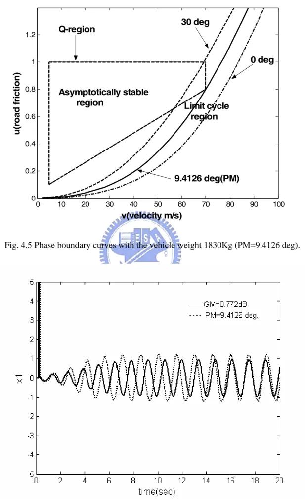
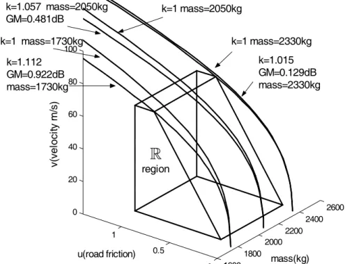
tester……….47 Fig. 4.2 The block diagram of the perturbed nonlinear system………47 Fig. 4.3 The limit cycle loci in the parameter plane……….48 Fig. 4.4 Gain boundary curves with the vehicle weight 1830Kg.(GM=0.772dB)…48 Fig. 4.5 Phase boundary curves with the vehicl weight 1830Kg (PM=9.4126 deg)…49 Fig. 4.6 Simulation results in time-domain with increased gain and phase………….49 Fig. 4.7 Gain boundary curves in 3-dimension………....50

Fig. 4.8 Phase boundary curves in 3-dimension………...50

Fig. 5.1 Single track vehicle model………..60

Fig. 5.2 Operating range………...61

Fig. 5.3 Block diagram of a fuzzy vehicle control system………...61

Fig. 5.4 Block diagram of a fuzzy vehicle control system………...61

Fig. 5.5 Membership functions of fuzzy controller………..62

Fig. 5.6 Control surface………62

Fig. 5.7 Limit cycle loci………63

Fig. 5.8 Time responses of input signal………63

Fig. 5.9 Stability boundary………...64

Fig. 5.10 Stability boundary………64

Fig, 5.11 GM and PM analysis………65

Fig. 6.1 The functional block diagram of PLL……….77

Fig. 6.2 The linearized mathematical model of PLL………77

Fig. 6.3 The closed feedback system with a gain-phase margin tester ke−jθ………..78

Fig. 6.4 The first order loop filter……….78

Fig. 6.5 The second order filter………79

Fig. 6.6 The 2D perturbed plane S with the perturbed parameters R₁ and C₁…..79

Fig. 6.7 The designed-parameter shaded area in k k -R_{d v 2} plane meeting the phase specifications PM≥30○ with the first order LF……….80

Fig. 6.8 The designed-parameter shaded area in k -R_{d 2} plane meeting the phase specifications PM≥30○ with kv =130000………80

Fig. 6.9 The bode plots of the PLL system at the vertices of the region S with 1 2 Q =(k R_d, )=(1.8,14Kohm) and k_v =130000……….81

Fig. 6.10 The designed-parameter shaded area in k -R_{v 2} plane meeting the phase specifications PM≥30○ with kd =0.6……….82

Fig. 6.11 The bode plots of the PLL system at the vertices of the region S with Q2 = 6 2 ( ,k Rv )= ×(3 10 , 5.1Kohm) and kd =0.6………..…82

Fig. 6.13 The designed-parameter shaded area in k k -R_{d v 2} plane meeting the phase specifications PM≥30○ with the second order LF……….83 Fig. 6.14 The designed-parameter shaded area in k -R_{d 2} plane meeting the phase specifications PM≥30○ and k_v =130000 with the second order LF………85 Fig. 6.15 The enlarged designed-parameter shaded area in k -R_{d 2} plane meeting the

phase specifications PM≥30○ and kv =130000 with the second order LF………85 Fig. 6.16 The bode plots of the PLL system at the vertices of the region R at

3 2

Q =(k R_d, )=(0.2, 60Kohm) and k_v =130000 with the second order LF………...86 Fig. 6.17 The designed-parameter shaded area in k -Rv 2 plane meeting the phase

specifications PM≥30○ and k_d =0.8 with the second order LF..87 Fig. 6.18 The enlarged designed-parameter shaded area in k -R_{v 2} plane meeting the phase specifications PM≥30○ and kd =0.8 with the second order LF…87 Fig. 6.19 The bode plots of the PLL system at the vertices of the region R at

4

4 2

List of Symbols

N describing function

φ phase shift

A amplitude of limit cycle ω frequency of limit cycle

k gain

θ phase

Φ input signal range of fuzzy logic S 2D perturbed parameter plane R 3D perturbed parameter space

Chapter 1

Introduction

1.1 Motivations

Gain margin and phase margin are important specifications in the frequency domain for

the analysis and design of practical control systems and have served as important measures of

robustness analysis which is always of primary concern. This is because the models used are

usually imprecise and the parameters of all physical systems vary with the operating

conditions and time. They are usually obtained numerically or graphically by the use of

system frequency response like Bode plots. Studying for controller design to satisfy GM, PM

or sensitivity conditions was proposed by several articles such as in [1]-[6], There are also

many design methods to determine the parameters to meet different objectives [7]-[9].

Designing a controller for a fixed and exact control plant is not usually practical in the natural

environments. Due to the simplified models or the factors resulting from the changing

environments, the uncertainties in system parameters can always occur. Uncertain parameters

stability of perturbed interval polynomials, is to guarantee if all the polynomials have the

roots in the left-half plane [17]. The perturbed parameters will result in root-clusters, within

which the roots of the perturbed polynomials will be located. Usually, a change in a physical

quantity typically appears in more than one coefficient of the characteristic equation. Robust

Gamma-stability analysis for a perturbed vehicle plant was also studied [18]. The methods of

analyzing the gain-phase margin of a linear control system with adjustable parameters have

been developed [19]-[21]. Strictly speaking, the majority of the researches mentioned above

are not concentrated on the controller design for perturbed systems. Sensitivity functions are

usually used as a design specification to indicate the robustness of a system. In [6] and [8],

Yaniv and Nagurka proposed a robust controller design method satisfying GM, PM and

sensitivity constraints on the perturbed systems, not with the system parameters in uncertain

continuous intervals, but with the system uncertainties in the finite discrete set of gains and

pole locations.

Undesirable oscillation phenomena due to nonlinearities in a feedback closed system

have been studied by many publications [22]-[26] and it is important for the designer to

predict the limit cycle behavior of a perturbed vehicle system with nonlinearities. It is of

interest to know the frequency, amplitude, stability and instability of the limit cycle occurred.

amplitude oscillations of closed nonlinear systems and has been successfully used in many

applications although some limitations exist in the systems which don’t satisfy the assumption

of filtering out the higher order harmonics [27]-[30].

In addition, some researchers have developed the experimental and analytic describing

functions of fuzzy controller in order to analyze the stability of fuzzy control systems [31-32].

Furthermore, the describing function technique to design a fuzzy controller for switching

DC-DC regulators was proposed by Gomariz et al [33]. The describing function was also

applied to find the bounds for the neural network parameters to have a stable system response

and generate limit cycles [34]. The results in [32] and [33] are extended to analyze the

stability of a fuzzy vehicle steering control system under the effects of system parameters and

gain-phase margin by the use of methods of describing function, parameter plane and a

gain-phase margin tester. A simple vehicle steering control model with perturbed parameters

is cited to verify the design procedure.

On the other hand, there are a large number of studies concentrated on the subject of

phase-locked loops (PLL) in the latest decades. The theoretical description of PLL was well

proposed [35]-[39]. A PLL is essentially a circuit that has a particular system lock its

frequency as well as the phase to those of the input applied to it. When the phase error is built

error is reduced to a minimum and a phase output of VCO is really locked to the reference

input. There are a considerable number of applications in many areas. A technique using PLL

was established on motor speed control [40]. In the design of Global Positioning System

receivers, PLL is very useful especially in a noisy environment [41]. PLL was also applied in

the design of frequency synthesizer [42].

In this thesis, GM and PM performances are defined for a perturbed system with

uncertain continuous interval parameters and shown here graphically in the system parameter

space. By the use of parameter space method and robustness stability criteria, stability

boundary curves corresponding to specific GM and PM constraints are generated. Owing to

the complexity of the controller design for perturbed control systems, it is not an easy job to

find out a qualified controller together with the system plant with uncertain interval

parameters so that the whole closed system at every point in the perturbed system parameter

region satisfies all the three specifications of GM, PM and sensitivity. The main concern in

the controller design is to find a desired region in the controller coefficient plane so that the

performance of the whole systemwith uncertain parameters inside a perturbed space satisfies

given specifications. The desired controller will be determined graphically from a figure in

which a qualified controller coefficient area is to be found out. With the help of stability

controller meeting the specified requirements is achieved.

1.2 Organizations of the Dissertation

The dissertation is organized as follows. Chapter 1 is an introduction. Basic concepts are

described in Chapter 2. In Chapter 3, a perturbed vehicle control system whose gain margin

(GM) and phase margin (PM) are analyzed and for which a novel controller design method

satisfying the given specifications on GM, PM and sensitivity is developed. In Chapter 4, the

subject of predicting the limit cycle of a nonlinear perturbed vehicle control system under

specific gain-phase margin (GM/PM) constraints is addressed. The analysis of robust stability

for a fuzzy vehicle steering control system is considered in Chapter 5. In Chapter 6, a control

algorithm is presented for phase-locked loop (PLL) design with perturbed parameters

satisfying frequency-domain specifications. In Chapter 7, conclusions are given and

Chapter 2

Basic Concepts

2.1 Overview

This chapter presents a description about the way how to analyze and design a feedback

control system with perturbed parameters varying in intervals by frequency approach.

Parameter space method and robust stability criteria provide a technique to check the stability

of perturbed control systems in a space with the coordinates of uncertain system parameters.

By the use of a gain-phase margin tester, stability boundary curves are generated to determine

gain and phase margins (GM and PM) in performance analysis. In the similar way, desired

controller coefficients are going to be found out to meet given specifications for controller

design. Sensitivity function is also considered in the controller design. With the nonlinearities

inherent in the system, describing function method is used for predicting limit cycle occurred.

2.2 Robust Stability Criteria

Consider the characteristic polynomial of a feedback control system

0 1 0 ( , ) ( ) ( ) ( ) ( ) n i n i n i P s q d q s d q d q s d q s = =

∑

where q=[ ,q q1 2,⋅⋅⋅⋅qn]∈ℜ and ℜ is a set of allowable parameter domain space. Each q i

varies independently within the interval with qi ∈[qi−;qi+],i= 21, ⋅ ⋅⋅n.

It has been shown that for real continuous coefficient functions di( )q of the characteristic equation, a sufficient condition for robust stability is that (a) there exists a

o

q=q ∈ℜ such that P s q( , ) is stable; (b) P s q( , ) doesn’t have any roots on the imaginary

axis for any q∈ℜ. It is easily tested by checking the stability of the characteristic

polynomial P s q( , o) for an arbitrary qo∈ ℜ. If no such qo exists, the system is unstable.

The condition (b) is satisfied if and only if the equation P s q( , )=0 neither has a real root at

0

s= , i.e.

0( )q 0

d ≠ (2.2)

nor an imaginary pair of roots at s= ±jω for all q∈ ℜ. Let ℜ be the set of all real q _jω such that the polynomial P s q has roots on the imaginary axis . ( , )

{ : ( , ) 0 for 0}

jω q P jω q ω

ℜ = = ≥ . (2.3)

The condition (b) also means that ℜ does not intersect the parameter domain space _jω

ℜ. The curve formed by the points q in ℜ in the _jω q−space is the stability boundary curve. The perturbed feedback control system is stable at the points in the q−space on one

side of the stable boundary curve and it is unstable at the points on the other side. The above

2.3 Describing Function

It is generally useful for the describing function technique to be applied in engineering

problems of control systems. Nonlinear systems are generally linearized by using the

describing function method to predict the limit cycle for stability analysis. Assume a

sinusoidal input x t( )= Asin(ωt) with the amplitude A and the frequency ω to a nonlinear system in Fig. 2.1 and y(t) is the output signal and periodic. By the Fourier series,

0 1 ( ) ( _nsin( ) _ncos( )), n y t a a n tω b n tω ∞ = = +

∑

∫

∫

∫

If the nonlinear system is symmetric about the origin, a₀ = . Let Y be a fundamental 0

component of the Fourier series of y(t) and Y= +a1 jb1= ∠Y1 θ1, where

2 2 1 1 1 Y = a +b and 1 1 1 1 tan b a θ ₌ −

. Y1 is the amplitude of the fundamental component of the system output y t( )

and θ is the phase shift by Fourier series.

The describing function N of a symmetric nonlinear system is defined as [28]

1 1 1 1 1 Y a jb N A θ A θ + = ∠ = ∠ (2.6)

Consider a perturbed closed control system with a gain-phase margin tester ke−jθ and there are r nonlinear components in the system. Every nonlinear component has the

complex describing function N (i i=1, 2,...., )r that is a complex function of A and ω,

which are the amplitude and frequency respectively of the input signal to the i−th nonlinear

element N and i

i iR iI

N =N + jN . (2.7)

Assume the closed characteristic equation is , 1 1I R I , 1 1I R I R I ( , , , , , , ..., ) the numerator of [1 ( , , , , ..., , ,..., )] 0, R r r j R m m r r P s q c k N N N N ke θG s q c N N N N N N θ − = + = (2.8) and , , 1 1I R I , , 1 1I R I 0 , , 0 1 1I R I 1 1 , , 1 1I R I ( , , , , , , ..., ) ( , , , , , ..., ) ( , , , , , ..., ) ( , , , , ,..., ) ( , , , , , ..., ) , R r r n t t R r r t R r r r n n R r r P s q c k N N N N d q c k N N N N s d q c k N N N N d q c k N N s d q c k N N N N s θ θ θ θ θ = = ∑ = + + ⋅⋅⋅ + (2.9)

where G s q c N( , , , _1R,N_1I,...,N_rR,N_rI) is an open loop transfer function of the system and c is a controller coefficient vector. c=[ , ,...c c_{0 1} c_m] and c is a controller coefficient to be _i designed for i=0,1, 2,...m.

, ,

1 1I R I

( , , , , , _R, ..., _{r r} )

P jω q c k θ N N N N may be written into the real part U( , , , , ,ω q c k θ N_1R,N_1I,. ,

R I)

..,Nr Nr and imaginary part V( , , , , ,ω q c k θ N1R,N1I,...,NrR,NrI).

, , 1 1I R I 1 1I R I 1 1I R I ( , , , , , , ,..., , ) ( , , , , , , ..., ) ( , , , , , , ,..., , ) R r r R r r R r r P j q c k N N N N U q c k N N N N jV q c k N N N N ω θ ω θ ω θ = + (2.10)

where 1 1I R I 0 1 1I R I 1 1 1I R I 2 2 1 1I R I 1 1I R I ( , , , , , , ,..., , ) ( , , , , ,..., , ) ( , , , , , ,..., , ) ( , , , , , ,..., , ) ( , , , , , ,..., , ) R r r R r r R r r R r r n n R r r U q c k N N N N r q k N N N N r q c k N N N N r q c k N N N N r q c k N N N N ω θ θ θ ω θ ω θ ω = + + + ⋅⋅⋅ + (2.11) and 1 1I R I 0 1 1I R I 1 1 1I R I 2 2 1 1I R I 1 1I R I ( , , , , , , ,..., , ) ( , , , , ,..., , ) ( , , , , , ,..., , ) ( , , , , , ,..., , ) ( , , , , , ,..., , ) . R r r R r r R r r R r r n n R r r V q c k N N N N i q k N N N N i q c k N N N N i q c k N N N N i q c k N N N N ω θ θ θ ω θ ω θ ω = + + + ⋅⋅⋅ + (2.12) The equations 1 1I R I 1 1I R I ( , , , , , , ,..., , ) 0 ( , , , , , , ,..., , ) 0 R r r R r r U q c k N N N N V q c k N N N N ω θ ω θ = ⎧ ⎨ ₌ ⎩ (2.13)

can be solved for q or for c.

2.4.1 Limit Cycle Prediction

For predicting the limit cycle resulting from nonlinearities N , (2.13) is solved for _i q given specific ω, , ,c k θ and A in system performance analysis analytically or numerically. Gain boundary curves will be generated from these q values in the q -parameter space by

varying ω given specific k and A with θ =0○ . Phase boundary curves will be

generated by varying ω given specific θ and A with k =1. Every boundary curve separates the parameter domain region into two areas as in Fig. 2.2. One is the asymptotically

system parameter point q is in the unstable area, but it won’t if q is in the stable area. The

gain and phase margins of the perturbed control system will be analyzed from boundary

curves geometrically. A specific gain or phase value corresponding to the boundary curve

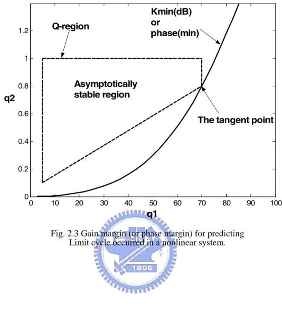
which is tangent to the perturbed parameter region as in Fig. 2.3 is defined as the GM and PM

of the perturbed system for predicting the limit cycles occurring, respectively.

2.4.2 GM Analysis without Nonlinearities

If there is no nonlinear part in a perturbed system, N1R,N1I,...,NrR, and NrI in (2.10)-(2.13) are omitted.

Equation (2.13) is rewritten into the following form ( , , , , ) 0 ( , , , , ) 0 U q c k V q c k ω θ ω θ = ⎧ ⎨ ₌ ⎩ (2.14) Equation (2.14) can be solved for q with specific ω, , ,c k θ . For gain margin analysis, a gain boundary curve is generated in q−space from the solutions q of (2.14) by varying ω for

every k with θ =0Ο. A specific gain k (dB) corresponding to the boundary curve which

is tangent to the perturbed region ℜ is defined as the GM of the perturbed control system. It is also the minimal GM of the system within the entire region ℜ. The GM of the control system at a point on one side of a specific gain boundary curve is greater than that at a point

on the boundary curve. But it is less at the points on the other side.

Equation (2.14) can be solved for q with respect to θ , given specific ω, ,c k. Phase boundary curves are developed under the PM specification in a similar way with k =1. They are generated in q−space from the solutions q of (2.14) by varying ω for every θ . The

PM of the control system is defined as the phase value θ associated with the phase boundary

curve which is tangent to the perturbed region ℜ. It is the minimal PM for the whole system with the parameters inside ℜ, too. The PM of the control system at a point on one side of a specific phase boundary curve is greater than that at a point on the boundary curve. But it is

less at a point on the other side.

2.4.4 Controller Design

The controller design is to determine the desired controller coefficients in selected c

-space. Based on gain-phase boundary curves drawn from the locations of the roots of (2.14)

for c and the constant-sensitivity loci, the desired area in c−space is found so that the

whole system with the controller in that area will meet specified conditions.

First, determine a gain region in c−space with the help of the gain boundary curves so that

the controller with the coefficients in that region satisfies the specified GM constraints.

Secondly, a phase-region is determined in c−space with the help of the phase boundary

curves so that the controller with the coefficients in that region satisfies the specified PM

The controller coefficients in that region will satisfy both the user-defined GM and PM

specifications.

2.5 Sensitivity Function

Sensitivity effects are often important to be considered in the design of control systems

on frequency domain and can be used as a design specification to indicate the robustness of

control system. The sensitivity function of the closed-loop transfer function H(s) with respect

to the variations of the transfer function G(s) which is a subsystem of H(s) is defined as ( ) ( ) ( ) / ( ) ( ) / ( ) H s G s H s H s S G s G s ∂ = ∂ (2.15) or with respect to the variations of an element β in H(s) is given by

( ) ( ) / ( ) / H s H s H s S_β β β ∂ = ∂ . (2.16)

2.6 Concluding Remarks

In this chapter, basic concepts of performance analysis and controller design for

perturbed control systems are addressed based on parameter space method and robust stability

criteria. GM and PM are analyzed and the desired controller is determined by the proposed

methods with the help of a gain-phase margin tester. Limit cycles are also predicted for

( )

cos

x t

=

A

ω

t

y t

( )

Fig. 2.1 A nonlinear system with input signal

x t

( )

=

A

cos

ω

t

0 10 20 30 40 50 60 70 80 90 100 0 0.2 0.4 0.6 0.8 1 1.2 Q-region Asymptotically stable region Limit cycle region q2 q1

Stability boundary curve

0 10 20 30 40 50 60 70 80 90 100 0 0.2 0.4 0.6 0.8 1 1.2 Kmin(dB) or phase(min) Q-region Asymptotically stable region

The tangent point q2

q1

Fig. 2.3 Gain margin (or phase margin) for predicting Limit cycle occurred in a nonlinear system.

Chapter 3

Robust Control Design for Perturbed

Systems by Frequency Domain Approach

3.1

Overview

The chapter presented here is concentrated on a perturbed vehicle control system whose

gain margin (GM) and phase margin (PM) are analyzed and for which a novel controller

design method satisfying the given specifications on GM, PM and sensitivity is developed.

The approach is applied to the plants with uncertain parameters that vary in intervals. Based

on the parameter space method and robust stability criteria, gain and phase boundary curves

are generated from the characteristic polynomial of the system with which a gain-phase tester

is included in series to perform system stability analysis and controller design. The main

concern in the controller design is to find a region in the controller coefficient plane so that

the performance of the uncertain system satisfies given specifications. The proposed method

is applied to an example of a bus system. Simulation results are given for illustration to show

the system performances on GM and PM and the desired controller meeting the specified

3.2 Sensitivity

Since in physical systems all the elements may change their properties with time and

environments, the considerations about the changes of the characteristics of the closed control

systems with respect to system parameter variations are always of big concern for a system

designer.

Consider a linear control feedback system illustrated in Fig. 3.1. The closed loop

feedback system has the transfer function given by

( , ) ( , ) ( , , ) 1 ( , ) ( , ) C s c G s q H s q c C s c G s q = + , (3.1)

where ( , )C s c is a controller with c=[ , ,...c c_{0 1} c_m] and c is a controller coefficient to be _i designed for i=0,1, 2,...m . G(s,q) is a plant with a perturbed parameter vector

1 2

[ , , _n]

q= q q ⋅⋅⋅⋅q ∈ℜ . ℜ is a set of allowable parameter domain space. Each q varies _i independently within the interval with q_i∈[q_i−;q_i+],i= 21, ⋅ ⋅⋅n.

Assume ( , ) ( , ) ( ) c c N s c C s c D s = (3.2) and ( , ) ( , ) ( , ) G G N s q G s q D s q = . (3.3)

With a specific q , H s q c is replaced by ( , , ) H s c .The sensitivity function ( , ) H( , )

i

s c c

respect to the controller coefficient c is defined as i ( , ) ( , ) / ( , ) / i H c i i s c dH s c H s c S dc c = , (3.4)

where i=0,1, 2....m. Substitute (3.1), (3.2) and (3.3) into (3.4), and the sensitivity function ( , )

i

H c

s c

S can be computed. Given a different constant s , the solutions of the equality ₀

( ) 0 H j i s j c S ω s ω

= = for a controller coefficient c give constant-sensitivity loci in the c−space. The controller coefficient c will be determined based on sensitivity specifications

corresponding to one of those loci. A system being very insensitive to parameter variations is

considered to be a good control system.

3.3 Stability Boundary Analysis

Consider a gain-phase tester ke−jθ included in series with the original control system as in Fig. 3.2, and its transfer function is given by

( , ) ( , ) ( , , , , ) 1 ( , ) ( , ) j j Ke C s c G s q H s q c K Ke C s c G s q θ θ θ = −₋ + . (3.5)

The characteristic polynomial is P s q c k( , , , , )θ and

0 0 1 ( , , , , ) the numerator of [1 ( , ) ( , )] ( , , , ) ( , , , ) ( , , , ) ( , , , ) j n i i i n n P s q c k ke C s c G s q d q c k s d q c k d q c k s d q c k s θ θ θ θ θ θ − = = + = = + + ⋅⋅⋅⋅ +

∑

By the use of the parameter space method and robust stability criteria, system stability

perturbed control systems in which the parameters of the characteristic polynomial lie within

given intervals, the minimum of all the GM values of the system at the points inside the entire

perturbed region in the parameter space is defined to be the GM of the system. The PM of the

system is defined in the same way.

3.3.1 Parameter Space Method

The parameter space method is a good analytical technique to perform system analysis in

the selected system parameter plane for a control system which is described by its

characteristic polynomial, the roots of which generate stability boundary curves in the

parameter plane. The characteristic polynomial on the jω-axis P j( ω, , , , )q c k θ may be

written into the real part U( , , , , )ω q c k θ and the imaginary part V( , , , , )ω q c k θ . ( , , , , ) ( , , , , ) ( , , , , ) 0 P jω q c k θ =U ω q c k θ + jV ω q c k θ = , (3.7) where 2 0 1 2 ( , , , , ) ( , , , ) ( , , , ) ( , , , ) n( , , , ) n U ω q c k θ =r q c k θ +r q c k θ ω+r q c k θ ω + ⋅⋅⋅ +r q c k θ ω (3.8) and 2 0 1 2 ( , , , , ) ( , , , ) ( , , , ) ( , , , ) _n( , , , ) n V ω q c k θ =i q c k θ +i q c k θ ω+i q c kθ ω +⋅⋅⋅+i q c k θ ω (3.9) The equations ( , , , , ) 0 ( , , , , ) 0 U q c k V q c k ω θ ω θ = ⎧ ⎨ ₌ ⎩ (3.10) can be solved analytically or numerically for q or c. Gain and phase boundary curves are

generated both in q−space from the solutions q for GM and PM analysis and in

space

c− from the solutions c for the controller design under specified conditions.

In the analysis of GM and PM, a fixed controller is used to analyze the system

performance, and (3.7)-(3.10) don’t depend on c. The gain and phase margins of the

perturbed vehicle system will be analyzed geometrically in 2 and 3 dimensions from stability

boundary curves.

In controller design, (3.10) can be solved for c with specific ω θ, ,k and q in a similar way. Gain and phase boundary curves are developed in the c−space according to

different gain k and θ , respectively.

3.3.2 Gain Margin Analysis

Let 0θ = Ο and c be a specific controller coefficient in Fig. 3.2. Equations (3.7) and

(3.10) are rewritten into the forms

( , , ) ( , , ) ( , , ) 0 P jω q k =U ω q k + jV ω q k = (3.11) and ( , , ) 0 ( , , ) 0 U q k V q k ω ω = ⎧ ⎨ ₌ ⎩ , (3.12) where 2 0 1 2 ( , , ) ( , ) ( , ) ( , ) n( , ) n U ω q k =r q k +r q k ω+r q k ω + ⋅⋅⋅ +r q k ω (3.13) and

2

0 1 2

( , , ) ( , ) ( , ) ( , ) n( , ) n

V

ω

ω

ω

ω

A gain boundary curve is generated in q−space from the solutions q of (3.12) by varying ω for every k. By varying k the curve is approaching to the parameter region ℜ gradually and finally intersect with ℜ. A specific gain k (dB) corresponding to the

boundary curve which is tangent to the parameter perturbed region ℜ is defined as the GM of the perturbed control system. It is also the minimal GM of the system within the entire

region ℜ. The GM of the control system at a point on one side of a specific gain boundary curve is greater than that at a point on the boundary curve. But it is less at the points on the

other side.

3.3.3 Phase Margin Analysis

Given k =1 and a specific c in Fig. 3.2, (3.7) and (3.10) are rewritten into the forms ( , , ) ( , , ) ( , , ) 0 P jω θq =U ω θq + jV ω θq = (3.15) and ( , , ) 0 ( , , ) 0 U q V q ω θ ω θ = ⎧ ⎨ ₌ ⎩ , (3.16) where 2 0 1 2 ( , , ) ( , ) ( , ) ( , ) _n( , ) n U ω θq =r qθ +r q θ ω+r qθ ω + ⋅⋅⋅ +r qθ ω (3.17) and 2 0 1 2 ( , , ) ( , ) ( , ) ( , ) _n( , ) n V

ω θ

θ

θ ω

θ ω

θ ω

Phase boundary curves are developed under the PM specification in a similar way. They are

generated in q−space from the solutions q of (3.16) by varying ω for every θ . The PM

of the control system is defined as the phase value θ associated with the phase boundary

curve which is tangent to the perturbed region ℜ. It is the minimal PM for the whole system with the parameters inside ℜ, too. The PM of the control system at a point on one side of a specific phase boundary curve is greater than that at a point on the boundary curve. But it is

less at a point on the other side.

3.3.4 Controller Design

The controller design is based on gain-phase boundary curves which are drawn in

space

c− from the locations of the roots of the polynomial equation (3.10) with respect to

different k and θ , and the constant-sensitivity loci which are drawn based on the solutions

of the H j( ) ₀

i _{s j}

c

S ω s

ω

= = for the controller coefficient c in c−space with respect to the given sensitivity constant s . The desired coefficients are determined under the constraints of 0

specified GM, PM and sensitivity. Systems with high stability and low sensitivity are desired.

Based on the discussions mentioned above, the design algorithm is as the followings:

Step 1: Set up user-defined specifications on GM, PM and sensitivity.

Step 2: For every system parameter q at the vertices of the perturbed system parameter

0dB in c-plane by solving (3.12).

Step 3: For every q at the vertices of the perturbed system parameter region in q -plane,

draw the phase boundary curves corresponding to the specified PM and 0○ in c-plane by

solving (3.16).

Step 4: Sketch the sensitivity constant loci from the solutions of the sensitivity equation

( ) 0 H j i _{s j} c S ω s ω = = for c, given s . 0

Step 5: Determine a gain region in c−space with the help of the gain boundary curves as in

step 2 so that the controller with the coefficients in that region satisfies the specified GM

constraints.

Step 6: Determine a phase-region in c−space with the help of the phase boundary curves as

in step 3 so that the controller with the coefficients in that region satisfies the specified PM

constraints.

Step 7: Find out the common region of the determined gain and phase ones as in steps 5 and 6.

The controller with the coefficients in that region is the desired one satisfying the specified

GM and PM conditions.

Step 8: Choose a point in c−space on a specified sensitivity constant locus which passes

through the common region as in step 7. Then the controller coefficient at that point satisfies

tradeoff has to be made among the three specified conditions.

3.4 An Example and Simulation Results

In this simulation, a Daimler Benz 0305 bus [18] is adopted. Its linearized system with

actuator input δ =steering angle rate, and output y=displacement of front antenna, has the

following transfer function

2 2 2 1 2 1 1 1 2 3 2 2 2 1 2 1 2 1 2 609.8 388600 48280 ( , , ) ( 1077 16.8 270000) q q s q s q G s q q s q q s q q s q q + + = + + + , (3.19)

where the parameter q₁ =v is the bus velocity, and the other parameter

u m q₂ = .

m: the mass of the bus (tons). u : road friction coefficient (0.5 for wet road, 1 for dry road).

1 1 1 2 [12 , 20 ] [24 ; 32 ] q ms ms q tons tons − − ∈ ∈ . (3.20) 3.4.1 GM and PM Analysis

The controller used is taken as given by

2 3 2 2344 10938 9375 ( ) 50 1250 15625 s s C s s s s + + = + + + (3.21) and was determined by Muench [18].

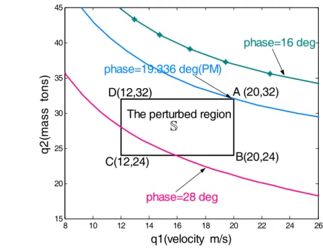
Case 1 : 2D GM/PM Analysis in q1−q Plane2 . Consider the system parameter q=[ ,q q1 2] with an uncertain parameter region S as in Fig. 3.3 for studying GM/PM performances.

The S−parameter region is

1 2 12 20 24 32 q q ≤ ≤ ⎧ ⎨ _{≤ ≤} ⎩ (3.22)

and the closed-loop characteristic polynomials is as in (3.6). By substituting s= jω into the

numerator of the above polynomials and by lengthy computation, the coefficients of the real

part polynomial U( , , , )ω q k θ with a specific c in (3.8) are 2 8 0 1 2 9 8 1 1 1 2 2 9 8 2 1 1 2 1 2 8 3 1 2 1 2 5 4 1 2 1 2 4.5262 10 cos( ), (3.6431 10 5.2808 10 ) sin( ), ( 4.2505 10 5716875 1.1316 10 ) cos( ), (6669992.4 9.1087 10 ) sin( ), 16828125 21000 3375 10 14293 r q k r q q k r q q q q k r q q q k r q q q q θ θ θ θ = × = × + × × = − × − − × × = − + × = + + × + 2 1 2 5 2 2 2 6 1 2 1 2 1 2 7 2 2 8 1 2 71.2 cos( ), 0, 1250 16.8 53850 270000, 0, . kq q r r q q q q q q r r q q θ = = − − − − = = (3.23)

In (3.9), the coefficients of the imaginary part polynomial V( , , , )ω q k θ are 2 8 0 1 2 9 8 1 1 1 2 2 9 8 2 1 1 2 1 2 2 3 1 2 1 2 8 1 4 4.5262 10 sin( ), (3.6431 10 5.2808 10 cos( ), (4.2505 10 5716875 1.1316 10 ) sin( ), 262500 4218750000 6669992.4 cos( ) 9.1087 10 cos( ) , 1429371.2 i kq i q kq i q q q q k i q q kq q k kq i θ θ θ θ θ = − × = × + × = × + + × × = − − − × − × = − 2 1 2 2 2 2 5 1 2 1 2 1 2 6 2 2 7 1 2 1 2 8 sin( ), 5 15625 840 1346250 135 10 , 0, 50 1077 , 0. kq q i q q q q q q i i q q q q i θ = + + + × = = − − = (3.24)

Solve the equations

( , , , ) 0 ( , , , ) 0 U q k V q k ω θ ω θ = ⎧ ⎨ ₌ ⎩ , (3.25) for q by varying k and θ , and the stable boundary representation curves for gain and

phase margins are shown as in Figs. 3.4 and 3.5 in the q1−q2 plane, respectively. We are only interested in positive solutions q₁ >0 and q₂ >0 for practical reasons. The GM of the perturbed control system with the domain region S is -4.3dB and its PM is 19.336○ as seen

in Figs. 3.4 and 3.5, respectively. In general, the specifications on the stability robustness

point of view are GM≥3dB and PM≥30○ , which the system with the original controller

(3.21) doesn’t satisfy. A new controller is designed in the following section and its

performance is improved significantly.

The gain boundary curves associated with different gains shown in Fig. 3.4 reveal that

the GM of the control system at a point on one side of a specific gain boundary curve is

greater than that at a point on the curve. But it is less at a point on the other side.

Similarly in Fig. 3.5, the phase boundary curves show that the PM of the control system

at a point on one side of a specific phase boundary curve is greater than that at a point on the

curve. But it is less at a point on the other side. At the point A (( ,q q1 2)=(20, 32)) in both Figs.3.4 and 3.5 the system has the minimal GM and PM of all the points within the entire S

region.

Case 2 : 3D GM/PM Analysis in m v u− − Space.

Select q=[ ,q q q1 2, 3] [ , , ]= m v u in the block diagram of the closed system in Fig. 3.2. The

24 / 32 12 20 0.5 1 m u v u ≤ ≤ ⎧ ⎪ _{≤ ≤} ⎨ ⎪ _{≤ ≤} ⎩ . (3.26)

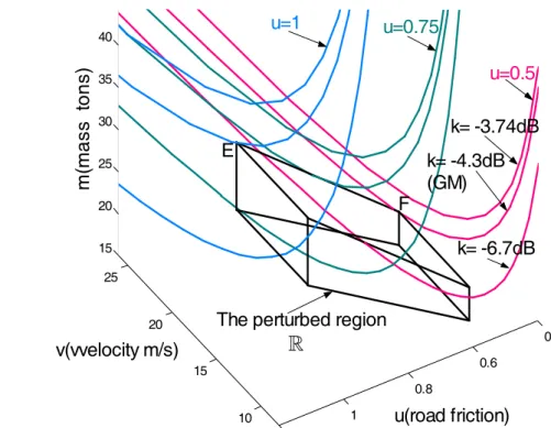
Gain and phase boundary curves in the m v u− − parameter space are generated from the solutions for q to (3.12) and (3.16), respectively. Those curves corresponding to

different k and θ by varying the frequency ω are shown in Figs. 3.7 and 3.8. A specific

gain k (dB) corresponding to a boundary curve which is tangent to the perturbed region R

at a point on the edge EF of R is defined as the GM of the system. It is also the minimal

GM of the perturbed control system within R . Its PM is defined in the same way. The

system with uncertain parameters within the R−space has GM=-4.3dB and PM =19.336○.

3.4.2 Controller Design

The system parameter q=[ ,q q_{1 2}] within S is considered for the controller design. Assume the controller to be designed is given as

2 2 1 0 3 2 ( ) 50 1250 15625 c s c s c C s s s s + + = + + + , (3.27) where c c₀, ₁ and c are the controller coefficients to be designed under the user-specified ₂

constraints and the system parameter domain is within the region S as in Fig. 3.3. Equation

(3.21) is a special case of (3.27) with c₀ =9375, c₁=10938 and c₂ =2344.

1) Controller Design for GM ≥3dB and PM ≥300

a coefficient region in c−space is to be found out by the use of gain and phase boundary

curves associated with different k and θ .

By solving (3.10), the coefficients of the real part of the characteristic polynomial

( , , , , ) U ω q c k θ in (3.8) are 2 0 0 1 2 1 0 1 1 1 2 2 2 1 1 0 1 2 2 1 2 3 1 1 2 2 1 2 5 4 1 2 1 2 2 1 2 2 5 48280 cos( ), (388600 48280 ) sin( ), (388600 609.8 48280 ) cos( ), (609.8 388600 ) sin( ), 16828125 21000 3375 10 , 609.8 cos( ), r c q k r c q c q k r c q c q q c q k r c q q c q k r q q q q q q c k r θ θ θ θ θ = = + × = − + + = − + = + + × + 2 2 2 6 1 2 1 2 1 2 7 2 2 8 1 2 0, 1250 16.8 53850 270000, 0, . r q q q q q q r r q q = = − − − − = = (3.28)

The coefficients of the imaginary part of the polynomial V( , , , , )ω q c k θ in (3.9) are 2 0 0 1 2 1 0 1 1 1 2 2 2 1 1 0 1 2 2 1 2 2 3 1 2 1 1 2 2 1 2 4 2 1 2 5 48280 sin( ), (388600 48280 ) cos( ), (388600 609.8 48280 ) sin( ) , 262500 4218750000 609.8 cos( ) 388600 cos( ), 609.8 sin( ), 15 i c q k i c q c q k i c q c q q c q k i q q c q q k c q k i c q q k i θ θ θ θ θ θ = − = + × = + + × = − − − × − = − = 2 2 2 1 2 1 2 1 2 5 6 2 2 7 1 2 1 2 8 625 840 1346250 135 10 , 0, 50 1077 , 0, q q q q q q i i q q q q i + + + × = = − − = (3.29)

where q=( ,q q1 2) is a specific point within S and (3.10) is rewritten into the following one.

( , , , ) 0 ( , , , ) 0 U c k V c k ω θ ω θ = ⎧ ⎨ ₌ ⎩ . (3.30) Two controller coefficients of c c and ₀, ₁ c₂ are chosen as adjustable parameters and the

other one is fixed for this design. By solving (3.30), a shaded area is determined by gain and

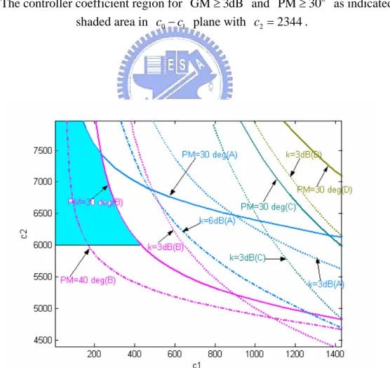
phase boundary curves from the solutions for ( , )c c pairs with _{0 1} c₂ =2344 under GM and PM specifications given as above in c0−c1plane, as shown in Fig. 3.9.

For the vertices A,B,C and D of S as in Fig. 3.3, stability boundary curves are plotted

to determine the qualified shaded area. Two gain boundary curves are obtained associated

with k=0dB and 3dB given θ =0○ for each vertex. In a similar way, two phase boundary ones are also generated corresponding to θ =0○ and θ =30○ with k=1.

Let c₀ =9375. Select c₁ and c₂ as adjustable coefficients. Gain and phase stability curves are generated in the same way in c1−c2 plane and the shaded region within which

1 and 2

c c satisfy specified constraints is founded, as shown in Fig. 3.10.

In Figs. 3.9 and 3.10 the desired controller coefficients can be chosen according to the

specified gain and phase constraints. The controller coefficient is selected from the above

shaded region so that the whole system with the chosen controller has the desired

specifications. With the designed controller, Tables 3.1 and 3.2 show the GM and PM of the

system operating at several points within the region S . The Bode plots of magnitude and

2) The constant-sensitivity loci

Compute ( , )

i

H s c c

S for i=0,1, 2 by substituting Eqs. (3.1)-(3.3) and (3.27) into (3.4) as

the followings: ( , ) 0 0 ( ) ( ) ( , )( ( ) ( ) ( , ) ( )) H s c c G c c G c G c c D s D s S N s c D s D s N s c N s = + , (3.31) ( , ) 1 1 ( ) ( ) ( , )( ( ) ( ) ( , ) ( )) H s c c G c c G c G c sc D s D s S N s c D s D s N s c N s = + , (3.32) and 2 ( , ) 2 2 ( ) ( ) ( , )( ( ) ( ) ( , ) ( )) H s c c G c c G c G c s c D s D s S N s c D s D s N s c N s = + . (3.33) Let c₂ =2344. The constant-sensitivity loci in Fig. 3.13, are plotted in c₀ −c₁ plane from the solutions to the equality ( ) 01

H j i s j

c

S ω s

ω

= = , where s is a specified sensitivity 01 constant and i=0,1. Gain and phase boundary curves in Fig. 3.11 are plotted with the system

operating at the point A in the region S . If the specified sensitivity locus passes through the

shaded area as in Fig. 3.9, a point on the locus is chosen and the controller at this location in

0 1

c − plane is desired. The point c Q1 on the sensitivity locus with the constraint

0 1 ( ) ( ) 0.001 H j H j s j s j c c S ω S ω ω ω =

= = = is chosen for the controller with c0 =180.7,c1=18.83 and

2 2344

c = . The system at the point A in S has GM=4.13dB and PM=37.1○ . Its performance on stability has been improved.

Let c0 =9375. The solutions to the equality ( ) 12 H j i s j c S ω s ω = = , where i=1, 2, give a plot of the constant-sensitivity loci in c₁−c₂ plane, as shown in Fig. 3.14. Choose the point

2

Q in Fig. 3.14 with c1 =410 and c1 =6000 on the sensitivity locus ₁ ( ) H j s j c S ω ω = = 2 ( ) 7 10 H j s j c S ω ω −

= = and the system operating at the point B in S has GM=6.08dB and PM=31○.

3.5 Concluding Remarks

This chapter introduces a new method on performance analysis and controller design by

frequency domain approach for a perturbed control system. Based on the parameter space

method and robust stability criteria, the performances of a perturbed vehicle control system

are analyzed in graphical portrayals. With the help of gain and phase boundary curves

resulting from the roots of the system characteristic polynomial equation, the GM and PM

have been obtained. In controller design, a methodology is proposed for portraying regions in

a selected controller coefficient plane so that the designed controller is to meet the specified

requirements on GM, PM and sensitivity. Simulation results demonstrate the objectives have

( , )

G s q

( )

C s

+

−

( )

s

δ

y s

( )

Fig. 3.1 The perturbed vehicle control system with uncertain parameter q .

+

_j

ke

−

θ

C s

( )

G s q

( , )

−

( )

s

δ

y s

( )

8 10 12 14 16 18 20 22 24 26 15 20 25 30 35 40 45 q1(velocity m/s) q2 (m ass t ons) A (20,32) B(20,24) C(12,24) D(12,32)

The perturbed region

S

Fig. 3.3 The parameter domain region S in q1-q2 plane.

8 10 12 14 16 18 20 22 24 26 15 20 25 30 35 40 45 q1(velocity m/s) q2 (m ass tons) A (20,32) B(20,24) C(12,24) D(12,32)

The perturbed region

K= -4.3dB(GM)

K= -3.1dB

K= -6.7dB

S

8 10 12 14 16 18 20 22 24 26 15 20 25 30 35 40 45 q1(velocity m/s) q2( m ass t ons) A (20,32) B(20,24) C(12,24) D(12,32)

The perturbed region

phase=16 deg

phase=19.336 deg(PM)

phase=28 deg S

Fig. 3.5 Phase boundary curves by varying θ with PM=19.336○.

8 10 12 14 16 18 20 22 24 26 _0. 0.6 0.7 0.8 0.9 1 1.1 1.2 15 20 25 30 35 40 u(road friction) v(velocity m/s) m( ma ss t o n s)

The perturbed region R

10 15 20 25 0 0.6 0.8 1 15 20 25 30 35 40 u(road friction) v(vvelocity m/s) m( ma ss t o n s) k= -3.74dB k= -4.3dB (GM) k= -6.7dB E F u=0.5 u=1 _u=0.75

The perturbed region

R

Fig. 3.7 Gain boundary curves in 3D with by varying k with GM=-4.3dB.

10 12 14 16 18 20 22 24 26 0.6 0.8 1 15 20 25 30 35 40 u(road friction) v(velocity m/s) m( ma ss t o n s)

The perturbed region

u=1 u=0.75 u=0.5 phase=28 deg. phase=19.336deg (PM) phase=16 deg E _F

R

Fig. 3.9 The controller coefficient region for GM≥3dB and PM≥300 as indicated in the shaded area in c₀− plane with c₁ c₂ =2344.

Fig. 3.10 The controller coefficient region for GM≥3dB and PM≥300 as indicated in the shaded area in c1−c2 plane with c0 =9375

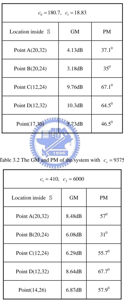
Table 3.1 The GM and PM of the system with c₂ =2344 0 180.7, 1 18.83 c = c = Location inside S GM PM Point A(20,32) 4.13dB 37.10 Point B(20,24) 3.18dB 350 Point C(12,24) 9.76dB 67.10 Point D(12,32) 10.3dB 64.50 Point(17,30) 5.73dB 46.50

Table 3.2 The GM and PM of the system with c_o =9375

1 410, 2 6000 c = c = Location inside S GM PM Point A(20,32) 8.48dB 570 Point B(20,24) 6.08dB 310 Point C(12,24) 6.29dB 55.70 Point D(12,32) 8.64dB 67.70 Point(14,26) 6.87dB 57.90

100 101 102 -50 0 50 100 101 102 -250 -200 -150 -100 Mag(dB) Phase (deg) A A B B C C D D Frequency(rad/sec)

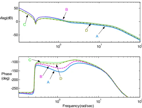
Fig. 3.11 Bode plots of magnitude and phase with c₀ =180.7,c₁ =18.83andc₂ =2344 at four vertices of the perturbed region S .

100 101 102 -50 0 50 100 101 102 -300 -250 -200 -150 -100 Mag(dB) Phase (deg) D D C C B B A A Frequency(rad/sec)

Fig. 3.12 Bode plots of magnitude and phase with c₀ =9375,c₁ =410 andc₂ =6000 at four vertices of the perturbed region S .

140 150 160 170 180 190 200 210 220 230 240 16 18 20 22 24 26 28 30 c0 c1 o k=0dB PM=19.336 deg s=0.001 PM=40deg. k=6dB k=3dB Q1 PM=30 deg

Fig. 3.13 A chosen controller at the point Q₁ with c₀ =180.7,c₁ =18.83 and c₂ =2344

based on the control system at the vertex A (20, 32) of the perturbed parameter region S .

100 200 300 400 500 600 700 800 5600 5800 6000 6200 6400 6600 6800 c1 c2 o k=3dB k=0dB k=6dB PM=30 deg. PM=40 deg. S12=10E(-7) Q2

Fig. 3.14 A chosen controller at the point Q₂ with c₀ =9375,c₁=410 and c₂ =6000