在混合自動重傳機制中設計位元交錯編碼調變及位元交錯編碼調變迭代解碼之適應性多重傳輸位元映射規則

(1)

國立交通大學

電信工程學系碩士班

碩士論文

在混合自動重傳機制中設計

位元交錯編碼調變及位元交錯編碼調變迭代解碼之

適應性多重傳輸位元映射規則

Adaptive Multiple Transmissions Mapping Design

for BICM and BICM-ID in HARQ

研究生：林哲群

指導教授：沈文和教授

(2)

在混合自動重傳機制中設計

位元交錯編碼調變及位元交錯編碼調變迭代解碼之

適應性多重傳輸位元映射規則

Adaptive Multiple Transmissions Mapping Design

for BICM and BICM-ID in HARQ

研究生 : 林哲群 Student : Che-Chun Lin

指導教授 : 沈文和博士 Advisor : Dr. Wern-Ho Sheen

國立交通大學

電信工程學系碩士班

碩士論文

A Thesis

Submitted to Department of Communication Engineering

College of Electrical and Computer Engineering

National Chiao Tung University

in Partial Fulfillment of the Requirements

for the Degree of

Master of Science

in

Communication Engineering

September 2008

Hsinchu, Taiwan, Republic of China

中華民國九十七年九月

(3)

在混合自動重傳機制中設計

位元交錯編碼調變及位元交錯編碼調變迭代解碼之

適應性多重傳輸位元映射規則

研究生: 林哲群指導教授: 沈文和教授

國立交通大學

電信工程學系碩士班

摘要

在文獻中已經指出，相較於使用同一位元映射規則於同一封包的多次傳輸，改變多次傳輸的位元映射規則可以提供更高的吞吐量。根據位元交錯編碼調變的通道容量分析，重傳時的位元映射規則必須隨著所操作的通道訊雜比的改變而改變。因此我們提出了使用基因演算法找出對每個訊雜比而言最好的位元映射規則。而當位元交錯編碼調變迭代解碼用在混合自動重傳機制時，由外來資訊轉換圖的分析也可得知，對同一編碼方式而言，每個不同的訊雜比也應該有不同的位元映射規則。因此我們在無限長度封包與無限迭代次數的假設下，針對每個訊雜比設計出最佳的位元映射規則。而在實際有限長度封包的應用下，我們畫出了解映射器與解碼器轉換圖相對於平均值的變動，同時建議在解映射器與解碼器的轉換圖之間保留一些空間來設計有限長度封包的位元映射規則。

(4)

Adaptive Multiple Transmissions Mapping Design

for BICM and BICM-ID in HARQ

Student: Che-Chun Lin

Advisor: Dr. Wern-Ho Sheen

Department of Communication Engineering

National Chiao Tung University

Abstract

It has been shown in the literature that varying bit-to-symbol mappings for multiple transmissions of the same packet provides better throughput performance compared to using the same bit-to-symbol mapping throughout all the transmissions. The analysis of BICM capacity suggests that the retransmission mapping scheme should be adaptive to the operating SNR. Hence we propose using a genetic algorithm to find the optimal mapping for each SNR. When BICM with iterative decoding (BICM-ID) is applied in HARQ systems, the analysis of EXIT-chart also suggests that the suitable mapping for each SNR for the same code should be different. Therefore, we find optimal mapping for each SNR under the assumption of infinite block length and unlimited iteration number. In the real application of finite block length, we plot the variation of demapper and decoder transfer curve relative to the averaged one and suggest that margins between the demapper and the decoder transfer curve should be preserved for the finite block length design.

(5)

誌謝

本篇論文的完成首先要特別感謝的是我的指導教授沈文和教授的細心指導，在每週定期的集會中不斷的提出問題，檢視每個想法中邏輯的缺失與漏洞，指出思考上的盲點，並提出有用的建議與指導，使本研究得以完善。同時也要感謝的是昌龍學長，在繁忙的工作之餘，還抽空一起討論研究，提出核心的關鍵問題，指出有價值的研究方向，並在遇到困難的過程中建議解決方法，是本研究能夠前進很大的助力。此外也要感謝實驗室其他的學長與同學們，在課業上互相討論研究，也提供了研究上的一些想法與啟發。當然也必須要感謝的是我的父母，提供一個舒適無慮的環境，使我能專心在課業上學習，不需擔憂生活，非常謝謝你們。最後，要感謝的是上帝，那所有慈悲、愛與恩典的泉源。民國九十七年九月研究生林哲群謹誌於交通大學

(6)

Content

摘要 ...iii

Abstract...iv

誌謝 ...v

Content ...vi

List of Tables ...viii

List of Figures...ix

Chapter 1: Introduction... 1

Chapter 2: Overview of HARQ ... 5

Chapter 3: System Model ... 8

3.1 Transmitter... 8

3.2 Channel... 9

3.3 Receiver ... 9

3.3.1 BICM Receiver Model ... 10

3.3.2 BICM-ID Receiver Model... 10

3.3.3 Joint MAP Demapper ... 11

Chapter 4: Symbol Mapping Diversity in HARQ ... 13

4.1 Constellations under joint detection ... 13

4.2 Coded Modulation Capacity... 16

4.3 Bit-Interleaved Coded Modulation Capacity... 23

Chapter 5: Extrinsic Information Transfer Chart... 28

5.1 Transfer characteristics ... 28

5.2 Transfer Characteristics of the Demapper ... 31

5.2.1 Demapper Transfer Function ... 31

5.2.2 Properties of the demapper transfer function ... 34

5.2.2.1 Area property ... 34

5.2.2.2 Zero prior characteristics ... 36

5.2.2.3 Summaries of the Properties of the Demapper Transfer Curve... 37

5.2.2.4 Some Examples of Demapper Transfer Curve ... 38

5.3 Transfer Characteristics of Decoder ... 40

5.4 Extrinsic Information Transfer Chart (EXIT Chart)... 43

Chapter 6: Mapping Design Criterion for BICM in HARQ... 45

6.1 Motivation ... 45

6.2 Design Criterion ... 47

Chapter 7: Mapping Design Criterion for BICM-ID in HARQ ... 48

7.1 Motivation ... 48

(7)

7.4 Distribution of Output Extrinsic Mutual Information ... 54

7.5 Design Criterion for finite block length ... 56

Chapter 8: Search Algorithm ...57

8.1 Simplified Model... 57

8.1.1 Hard-decision Virtual Channel ... 57

8.1.2 Extrinsic Channel ... 60

8.1.3 Closed Form Demapper Transfer Function ... 61

8.2 Genetic Algorithms... 62 8.2.1 Introduction ... 62 8.2.2 General Procedure ... 64 8.2.3 Representation Scheme... 65 8.2.4 Selection ... 66 8.2.5 Crossover ... 66 8.2.6 Mutation ... 67 8.2.7 Suggested GA Parameters ... 68 8.2.7.1 Population Size ... 68 8.2.7.2 Elite Number ... 69 8.2.7.3 Crossover Probability ... 70 8.2.7.4 Mutation Probability... 71

8.2.7.5 Summary of the Suggested GA Parameters... 72

Chapter 9: Mapping Search Results ... 73

9.1 Mappings for BICM ... 73

9.2 Mappings for BICM-ID with infinite block length ... 79

9.3 Mappings for BICM-ID with finite block length ... 82

Chapter 10: Simulation Results ... 84

10.1 BICM ... 84

10.1.1 Turbo Codes... 87

10.1.2 Convolutional Codes ... 92

10.2 BICM-ID ... 95

10.2.1 Mappings for Infinite Block Length... 95

10.2.2 Mappings for Finite Block Length ... 97

Chapter 11: Conclusions... 99

(8)

List of Tables

Table 9.1.1 BICM mappings (T=2): ... 74

Table 9.1.2 BICM mappings (T=3) ... 77

Table 9.2.1 BICM-ID mappings for infinite block length (T=2, 1st) ... 79

Table 9.2.2 BICM-ID mappings for infinite block length (T=2, 2st) ... 80

Table 9.3.1 BICM-ID mappings for finite block length (T=1)... 82

Table 9.3.2 BICM-ID mappings for finite block length (T=2,1st) ... 83

(9)

List of Figures

Fig 3.1 BICM in HARQ transmitter model... 8

Fig 3.3.1 BICM in HARQ receiver model ... 10

Fig 3.3.2 BICM-ID in HARQ receiver model... 10

Fig 4.1.1 constellations with Gray mapping for the first transmission ... 13

Fig 4.1.2 constellations with the same mapping as the first transmission for the second transmission... 13

Fig 4.1.3 constellation under joint detection ... 14

Fig 4.1.4 re-mapping for the second transmission ... 14

Fig 4.1.5 constellation after re-mapping... 15

Fig 4.2.1 CM capacity of different mapping schemes... 21

Fig 4.2.2 distance distribution of different mapping schemes... 22

Fig 4.3.1 Equivalent parallel channel model for BICM in the case of ideal interleaving ... 24

Fig 4.3.2 BICM capacity of different mapping schemes... 27

Fig.5.1.1 iterative demapping and decoding model... 28

Fig 5.2.2.1 Binary Erasure Channel ... 34

Fig 5.2.2.2 Properties of the Demapper Transfer Curve... 37

Fig 5.2.2.4.1 Various demapper transfer curve at the same SNR (T=1)... 38

Fig 5.2.2.4.2 demapper transfer curve at different SNR (T=1) ... 39

Fig 5.2.2.4.3 Various demapper transfer curve at the same SNR(T=2)... 40

Fig 5.3.1 decoder transfer curve of different codes ... 41

Fig 5.3.2 decoder transfer curve of different code rate ... 41

Fig 5.3.3 decoder transfer curve of turbo code with different iteration number ... 42

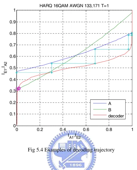
Fig 5.4 Examples of decoding trajectory... 44

Fig 6.1 BICM capacity for various mapping schemes ... 46

Fig 7.1.1 different decoder and demapper transfer curve... 48

Fig 7.1.2 mappings at different SNR ... 49

Fig 7.3.1 Decoding trajectory for finite block length ... 51

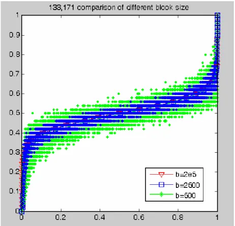
Fig 7.3.2 Variation of decoder transfer curve for different block length ... 52

Fig 7.3.3 Variation of demapper transfer curve for different block length... 53

Fig. 7.4.1 Distribution of demapper transfer curve ... 54

Fig 7.4.2 Distribution of decoder transfer curve ... 55

Fig.8.1 simplified channel model ... 57

Fig 8.1.1 CM capacity of real channel and virtual channel (T=2) ... 59

Fig 8.1.2 binary erasure channel... 60

(10)

Fig 8.1.3.2 Various virtual and real channel demapper (T=2) ... 62

Fig 8.2.2 Flow chart for genetic algorithm... 64

Fig 8.2.3 8 PSK constellation ... 65

Fig 8.2.5 crossover operation ... 67

Fig.8.2.6 mutation operation ... 67

Fig 8.2.7.1 population size comparison... 68

Fig 8.2.7.2 elite number comparison ... 69

Fig 8.2.7.3 crossover probability comparison ... 70

Fig 8.2.7.4 mutation probability comparison ... 71

Fig 9.1.1 16QAM constellation ... 73

Fig 9.1.2 BICM capacity of mappings designed for different SNR (T=2)... 75

Fig 9.1.3 Comparison of BICM capacity of different mapping schemes (T=2) ... 76

Fig 9.1.4 BICM capacity of mappings design for different SNR (T=3) ... 78

Fig 9.1.5 Comparison of BICM capacity of different mapping schemes (T=3) ... 78

Fig 9.2.1 demapper transfer function for inifinite block length (T=1) ... 81

Fig 9.2.2 demapper transfer function for inifinite block length (T=2) ... 81

Fig 9.3.1 demapper transfer curve for finite block length (T=1)... 82

Fig 9.3.2 demapper transfer curve for finite block length (T=2)... 83

Fig 10.1.1.1. Throughput of turbo code with code rate=1 3, T=2 ... 87

Fig 10.1.1.2 Throughput of turbo code with code rate=1 3, best candidates, T=2 ... 87

Fig 10.1.1.3 Throughput of turbo code with code rate=1 2, T=2 ... 88

Fig 10.1.1.4 Throughput of turbo code with code rate=1 2, best candidates, T=2... 88

Fig 10.1.1.6 Throughput of turbo code with code rate=3 4, best candidates, T=2... 89

Fig 10.1.1.8 Throughput of turbo code with code rate=1 3, best candidates T=3 ... 90

Fig 10.1.1.10 Throughput of turbo code with code rate=3 4, best candidates T=3... 91

(11)

Fig 10.1.2.1 Throughput of convolutional code with code rate=1

3, T=2 ... 92 Fig 10.1.2.2 Throughput of convolutional code with code rate=1

3, best candidates,

T=2 ... 92 Fig 10.1.2.3 Throughput of convolutional code with code rate=1

2, T=2... 93 Fig 10.1.2.4 Throughput of convolutional code with code rate=1

2, best candidate,

T=2 ... 93 Fig 10.1.2.5 Throughput of convolutional code with code rate=3

4, T=2... 94 Fig 10.1.2.6 Throughput of convolutional code with code rate=3

4, best candidates,

T=2 ... 94 Fig 10.2.1.1 BER of different block length ... 95 Fig 10.2.1.2 Throughput of block length =2500... 96 Fig 10.2.2.1 BER comparison of finite length demapper and infinite length

demapper (T=1) ... 97 Fig 10.2.2.2 Throughput comparison of finite length demapper and infinite length

(12)

Chapter 1: Introduction

One of the main challenges in wireless communication is the fluctuation of signal amplitude caused by fading. Many efforts have been put to mitigate this adverse effect. Trellis coded modulation (TCM), originally proposed by Ungerboeck for bandwidth- efficient communication over the additive white Gaussian noise (AWGN), has shown some drawbacks when transmitting over fading environment. In the design of TCM, modulation and coding is combined as an entity to improve the performance. The design goal is to maximize the minimum free Euclidean distance, and therefore it is often optimized over AWGN channel. However, when transmitting over fading channels, its performance is significantly degraded since the diversity order is usually low. To combat the adverse effect of fading channel, symbol interleaver is added and parallel transitions in the trellis should be avoided. However, since the minimum number of distinct symbols between two codewords limits the diversity order, the constraint length should be increased. The increased constraint length further results in exponentially increased decoding complexity which is unacceptable.

In [2], Zehavi proposed an alternative approach called bit-interleaved coded modulation (BICM) to increase the diversity order to the minimum Hamming distance of the code. By placing a bit-wise interleaver at the encoder output, this allows large diversity order with moderate system complexity. In [4], Li and Ritcey showed that the performance of BICM can be further improved by iterative decoding between the demapper and the decoder, a scheme called bit-interleaved coded modulation with iterative decoding (BICM-ID). It has been shown in the literature that the design of the demapper is crucial to achieve a high coding gain over iteration. In [6], EXIT chart was proposed to describe the iterative decoding behavior through a decoding trajectory between the transfer curve of the demapper and decoder.

(13)

On the other hand, error control is also a main issue for data communication. Combined with the advantage of automatic-repeat-request (ARQ) mechanisms and forward-error-correction (FEC) schemes, HARQ is often adopted to achieve high reliability and high system throughput. In HARQ schemes, additional redundant parity bits are appended to the original message for both error correction and detection. When the presence of errors is detected, the receiver first tries to correct the erroneous bits. If the number of errors is beyond the designed error-correcting capability of the code, a retransmission request is send to the transmitter. The retransmitted packets can be exactly the same as the initial one or contain some extra redundant bits. When a new packet is received, the newly received packet can be decode alone or jointly decode with the previous ones.

In this thesis we are concerned about the case that retransmission carry identical bits and all the received packets are combined together for decoding. Furthermore, BICM and BICM-ID in conjunction with HARQ is considered.

It is known that the performance will be significantly improved by introducing packet combing. Chase combining [12] is the well known ML combing technique. It combines arbitrary number of coded packets into a single coded packet with lower code rate, thus improves the error-correcting capability of the code. However, Wengerter [15] showed that different bit to symbol mapping for retransmission can further improves the system performance. By simply swapping or taking logic inversion on the modulation bits to average out the unequal bit reliabilities, a method called constellation rearrangement, significant improvement has been observed. However, no optimality can be claimed on this method. In [16], an optimization criterion base on the BER upper bound has been proposed. The main deficiency of the mapping found by the minimization of the BER upper bound is that the upper bound is only tight at high SNR, the performance at low SNR can not be guaranteed. Murthy

(14)

[17] further suggested to change the criterion to maximize the sum of the magnitudes of the LLR of the bits forming the M-QAM symbols in different retransmissions. However, the maximization is made on the sum not on the individual bits LLR, no optimality can be guaranteed. Another criterion based on the augmented signal space after retransmission is to maximize the minimal accumulated (over transmission) squared Euclidean distance [18]. Gidlund [19] also aimed at increasing the Euclidean distance between signal points, thus applying the idea of set-partition in TCM to spread the signal points well in the augmented signal space. These designs ignore the relationship of the number of bit differences between nearest symbols; however, the number of bit differences is a crucial parameter for the design of BICM mappings. Hence is also not optimized for BICM systems.

Those mapping designs described above are all independent of SNR. However, an analysis based on the BICM capacity under multiple transmission [14] showed that one single mapping can not be optimal for the whole interested SNR range. It was showed that constellation rearrangement (CoRe) outperforms the mapping obtained by the minimization of BER upper bound (MBER) at low SNR. However, at high SNR, MBER exhibits better performance than CoRe. Since there are different operating SNR region at different code rate, this paper suggests that mapping should be adaptive considering the targeted spectral efficiency (code rate). Although adaptive mapping scheme has been proposed, mappings that are optimized for each SNR is still an open problem. Hence we aim to find these optimal mappings.

When iterative decoding is applied (BICM-ID), mapping design is especial crucial for obtaining large iterative decoding gain even for single transmission. Various mapping design methods have been proposed for single transmission. However, very few have addressed the issue of multiple transmissions mapping design. In [21],

(15)

pairwise error probability and the uncoded ideal prior pair-wise error probability. Since the uncoded pair-wise error probability is independent of the underlying coding scheme, the design is not optimized for a particular code and may cause large performance degradation. By the analysis of the EXIT chart, the first intersection of the demapper transfer curve and the decoder transfer curve should be as high as possible. Since different mapping and coding have different transfer curve, their first intersection will be different. Therefore, a mapping that is good for a particular code may not be good for another one as well. Guided by the EXIT chart, mapping design should be dependent on the outer code. Furthermore, the dependency of the demapper transfer function on SNR also suggests that different mappings should be designed for the same code on different SNR. Hence we propose a method jointly considering the outer code and the operating SNR to design the retransmission mappings based on the EXIT chart.

(16)

Chapter 2: Overview of HARQ

A major concern in data communication is how to control transmission errors caused by the channel noise so that error-free data can be delivered to the user. There are two basic error-control schemes for data communication: automatic-repeat-request (ARQ) schemes and forward-error-correction (FEC) schemes.

In an ARQ error-control system, some parity bits are appended to the original information bits for error detection. When a codeword is received, the receiver computes its syndrome and determines if there is any erroneous bit. If the presence of errors is detected, the receiver discards the erroneously received codeword and requests a retransmission of the same codeword via a feed back channel.

In an FEC error-control system, an error-correcting code is used for combating transmission errors. When the receiver detects the presence of errors in the received codeword, it attempts to correct them. After the error correction has been performed, the decoded codeword is then delivered to the users. If the receiver failed to detect the presence of errors or the number of erroneous bits exceeds the error-correcting capability of the code, a decoding error is committed.

The advantages of ARQ scheme is simple and provides high system reliability. However, the throughput of ARQ system falls rapidly with increasing channel error rate. On the contrary, the FEC schemes maintain constant throughput (equal to the code rate) but is less reliable since the decoded message has to be delivered to the user regardless of whether it is correct or not. Thus to overcome the drawbacks in both ARQ and FEC schemes, a combination of these two called hybrid automatic-repeat-request (HARQ) scheme is proposed.

(17)

errors are detected by the receiver, the receiver tries to correct the erroneous bits. If the receiver fails to correct all of them, a retransmission request is delivered to the transmitter. The system throughput is increased by correcting the error patterns that occur most frequently. The system reliability is increased by requesting a retransmission rather than passing the unreliably decoded message to the user. As a result, a proper combination of FEC and ARQ provides higher throughput than FEC system and higher reliability than ARQ system.

There are three types of HARQ scheme, type I, type II and type III. In type I HARQ scheme the uncorrectable error packets are simply discarded and the receiver requests a retransmission of the same packet. Type I scheme is suitable for fairly static channel conditions since the error-correcting code can be designed specifically for this constant noise level. However, in applications with fluctuating channel conditions, type I has some drawbacks. When the bit error rate is small such that only small error correction capability is needed, the redundancy bits carried for correction of large bit errors represent a waste. When the channel is very noisy, the possibility of inadequate error-correcting capability will increase the frequency of retransmission and hence reduces the system throughput.

To overcome the drawbacks of the type I scheme, incremental redundancy HARQ (IR-HARQ) scheme is proposed. The basic idea is to transmit the additional redundancy bits only when they are needed. When the channel condition is good, only a small fraction of redundancy bits are transmitted to correct small bit errors. When a retransmission request is delivered to the transmitter, additional redundancy bits are transmitted to the receiver. The receiver than combine the newly received packet and the previous ones to form a more powerful code with lower effective code rate. These schemes offer higher throughput efficiency since the error correcting code redundancy is adapted to the varying channel conditions. Depending on whether each retransmitted

(18)

packets are self decodable or not, IR-HARQ can be further categorized into two classes: type II and type III schemes. Type II scheme is also referred to as full incremental

redundancy scheme where only incremental redundancy bits to the initial transmission are retransmitted. Type III scheme is also referred to as partial incremental redundancy scheme where partly identical bits and partly incremental bits to the initial transmission are retransmitted. The main drawback of type II scheme is that the decoder has to rely on both the previous received packets as well as the newly received one to decode. In situation where a packet may be lost, it is not possible to use previous packet and recover the original message. Thus it is desirable to have a scheme where incremental coded bits are self decodable.

Another advantage that makes type II and type III HARQ scheme more attractable than type I is that instead of simply discard the erroneous packets, type II and type III scheme combine the previous received packets and jointly decode them. Although damaged by the channel noise, these packets still carry useful information that is beneficial for decoding. Therefore, decoding with packet combining often performs better than decoding without packet combining.

(19)

Chapter 3: System Model

3.1 Transmitter

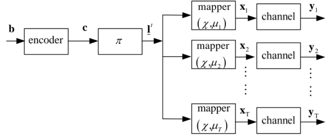
Fig 3.1 BICM in HARQ transmitter model

Consider the system model described by Fig3.1. A vector of binary bits

1 2 [ , ,..., ] I N b b b =

b with lengthN is encoded to binary codewords _I =[ ,₁ ₂,..., ]

c

N

c c c

c

with length N . The encoded codewords are then fed into bit interleaver _c π . The

interleaved codewords are denoted as [ , ,...,₁ ₂ ]

L t t t t N = l l l l , where [ _,1, _,2,..., _, ] s t t t t i = li li li n l

,i=1,....,N_L is a group of n bits that will be mapped to a complex symbol. The _s

sequence of 2ns_{-ary complex symbols are denoted as}

,1 ,2 , [ , , , ] L i i i N x x x = i x … . The first

subscript indicates the i-th transmission ,i=1,....,T , and T is the maximum allowed

transmission number. Since different bit to symbol mappings can be adopted while retransmission, we denote the i-th transmission mapper asμ_i and , 1

( )

t

i k k

x =μ l ∈χ.

In our notation convention, we write random variables using upper case letters and their realizations by the corresponding lower case letters. Bold case letters represent vectors and underscore is used to represent a sequence of vectors. The same terminology will be used throughout this thesis.

b c π

(

1

)

mapper , χ μ

(

2

)

mapper , χ μ

(

)

mapper , _T χ μ encoder t l 1 y 1 x 2 x T x 2 y T y

(20)

3.2 Channel

The signal x_i is send over the channel and y_i =h x_i T_i +n_i is the received one, where [ _,1, _,2,...., _, ] L i = ni ni ni N n is AWGN and [ _,1, _,2,..., _, ] L i i i N h h h = i h is the channel

fading gain. Each elements in n_i is an iid complex Gaussian Random variable with zero mean and variance 0

2

N

in real and imaginary part. When the channel is modeled as a frequency non-selective fast fading channel,h_{i k}_, is an iid complex Gaussian random variable with zero mean and variance 1

2 in real and imaginary part. When the channel is modeled as an AWGN channel, h_{i k}_, is 1 for all i and k. Finally, we assume that SNR is the same for each retransmission.

3.3 Receiver

Here we denote

( )

,

(

₁

( )

, , ₂

( )

, ,...,

( )

,

)

L N u v = u v u v u v L L L L as a sequence of log

likelihood ratio (LLR), where u∈{ , , },D A E v∈{ , }φ ϕ . D stands for Detection, A for a priori, and E for extrinsic.φ stands for the demapper and ϕ for the decoder.

( )

, { ,1

( )

, , ,2

( )

, ,...., , _s

( )

, }

k u v = Lk u v Lk u v Lk n u v

L is a sequence of LLRs belong to the

k-th symbol {x_1,_k,x_2,_k,....,x_{T k}_, } (Since the same coded bits are transmitted in each retransmission, each k-th symbol carries the same coded bits.)

(21)

3.3.1 BICM Receiver Model

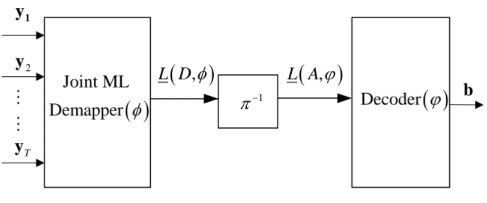
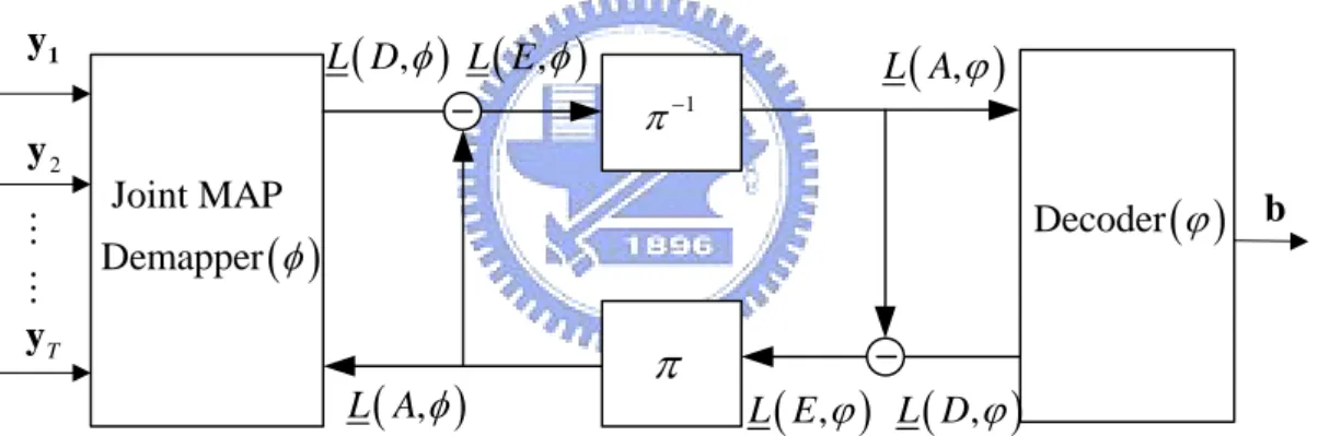
Fig 3.3.1 BICM in HARQ receiver model

As shown in Fig 3.3.1, the joint ML demapperφ receives a sequence of symbols

1, 2,..., T

y y y in all T transmissions and jointly detects them to compute the coded bit LLRs L

(

D,φ

)

for the decoder. After passing through the deinterleaver π−1 to restore the original bit order, the deinterleaved LLRL

(

A,φ

)

is fed into the decoder. The original information bitsbare then decoded by the decoder.

3.3.2 BICM-ID Receiver Model

Fig 3.3.2 BICM-ID in HARQ receiver model

When iterative decoding is applied, the demapper not only receives the T transmission symbols y y₁, ₂,...,y_T but also the a priori information L

(

A,φ

)

generated by the decoder. The demapper then apply MAP detection algorithm to

( )

Joint MAP Demapper φ

( )

Decoder ϕ

π

1 y 2 y T y

(

,

)

L E φ _{L A}

(

_,_ϕ

)

(

,

)

L Aφ L E

(

,ϕ

)

b

(

,

)

L D φ

(

,

)

L D ϕ 1 π−

( )

Joint ML Demapper φ Decoder

( )

ϕ 1 y 2 y T y

(

,

)

L Aϕ b

(

,

)

L Dφ 1 π−

(22)

compute the coded bit LLRs L

(

D,φ

)

. Before passing to the decoder, the demapper subtracts the a prior information L

(

A,φ

)

to produce the extrinsic information

(

E,φ

)

L . The decoder applies similar pricinple to generate the extrinsic information

(

E,ϕ

)

L and feed back to the decoder. Thus the signal is iteratively decoded by mutually exchanging soft information between inner demapper and outer decoder. This iteration process continues until a prescribed number of iteration is reached.

3.3.3 Joint MAP Demapper

The demapper computes the a posteriori probability for coded bits. Since the modulation is memoryless, only the k-th symbol is concerned when detecting the i-th bit in the k-th symbol. Therefore, for simplicity, we drop the subindex k in the k-th label l and definet_k

(

₁, ,...,₂

)

(

_,1, _,2,..., _,

)

s s

t t t t t t t t

n k k k k n

l l l l l l

= =

l l ∈ Λ .For the i-th bit LLR in

the k-th symbol, define L u v_i

( )

, L_{k i}_,

( )

u v, . Similarly, we define

, , , , , , ,

i i k i i k i i k i i k

x x y y h h n n , and therefore y_i =h x_i _i+ . Perfect channel state n_i

information is assumed at the receiver, thus the LLR for the i-th bit is calculated as

(

)

₍

(

)

₎

(

)

(

)

(

)

(

)

1 2 1 2 1 2 1 2 1 2 1 2 1 2 1 2 1 2 T 1 2 1| , ,..., , , ,..., , log 0 | , ,..., , , ,..., 1 , ,..., | 1 , ,..., | 1, , ,...,

log log log

0 , ,..., | 0 , ,..., | 0, , ,..., t i T T i _t i T T t t t i T i T i T t t t i T i i T p l y y y h h h L D p l y y y h h h p l p h h h l p y y y l h h h p l p h h h l p y y y l h h h φ = = = = = = = + + = = =

(

)

(

)

(

)

(

)

(

)

1

(

)

1 2 1 2 1 2 1 2 1 2 T 1 2 1 2 1 2 1 2 1 2 1 , ,..., , ,..., | 1, , ,...,

log log log

, ,..., 0 , ,..., | 0, , ,..., , ,..., , | 1, , ,..., , log , ,..., , | 0, , ,..., i t t i T T i T t t T i i T t t T i T i t t T i p l p h h h p y y y l h h h p h h h p l p y y y l h h h p y y y l h h h L A p y y y l h h h φ ∈Λ = = = + + = = = = + =

∑

t l l l

(

)

0 t i T ∈Λ

∑

l

(23)

(

)

( )

(

)

(

)

( )

(

)

(

)

(

)

( )

₍

₎

1 0 2 2 1 1 2 2 1 1 2 2 1 1 || || exp 2 0 , log || || exp 2 0 || || exp exp , 2 , log s t i s t i s t _n t T k k k j j t k j _j j i i _t _t n T k k k j j t k j j j i t _n T k k k j j k j i j i y h p l c p l L A y h p l d p l y h c L A L A μ σ φ μ σ μ φ σ φ = = ∈Λ ≠ = = ∈Λ ≠ = ≠ = ⎛ − ⎞ = ⎜− ⎟ ⎜ ⎟ ₌ ⎝ ⎠ = + ⎛ ₋ ⎞ ₌ ⎜− ⎟ ⎜ ⎟ ₌ ⎝ ⎠ ⎛ − ⎞ ⎜− ⎟ ⋅ ⎜ ⎟ ⎝ ⎠ = +

∑

∏

∑

∏

∑

l l l l l

( )

₍

₎

1 0 2 2 1 1 || || exp exp , 2 t i s t i t _n T k k k j j k j i j y h d L A μ φ σ ∈Λ = ≠ ∈Λ = ⎛ ⎞ ⎜ ⎟ ⎜ ⎟ ⎜ ⎟ ⎝ ⎠ ⎛ ⎞ ⎛ − ⎞ _⎜ _⎟ ⎜− ⎟ _⎜ ⋅ _⎟ ⎜ ⎟ _⎜ _⎟ ⎝ ⎠ _⎝ _⎠

∑

l l l

(24)

Chapter 4: Symbol Mapping Diversity in HARQ

4.1 Constellations under joint detection

When the same mappings are used during further retransmissions, the performance improvement comes only from SNR gain. If the same signal is transmitted T times, 3T dB gain will obtained at the receiver. However, when the retransmission mappings are changed, the receiver will have the potential to get not only 3T dB gain but also additional gain by the benefit of symbol mapping diversity. This can be well explained by the enlarged signal space under joint detection. For the simplicity of exposition, consider 4-PAM transmission in the following:

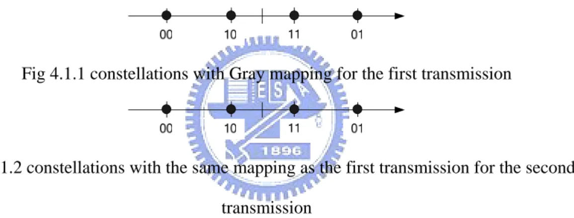
Fig 4.1.1 constellations with Gray mapping for the first transmission

Fig 4.1.2 constellations with the same mapping as the first transmission for the second transmission

In our first example (Fig 4.1.1 and Fig 4.1.2), Gray mapping is transmitted at the first time and the same mapping is adopted at the second transmission. Since the receiver receives two signal and jointly detect them, the signal space under joint detection is enlarged to two times the dimension of single transmission. As shown in Fig 4.1.3, the signal space is now a two dimensional one instead of just one dimension.

(25)

Fig 4.1.3 constellation under joint detection

The abscissa in Fig 4.1.3 represents the constellation for the first transmission and the ordinate represents the one for the second transmission. Let us denote the minimum Euclidean distance between the constellation points in single transmission as d . Then ₁

the minimum Euclidean distance after the second transmission will be

2 2

2 1 1 2 1

d = d +d = d Therefore the SNR is doubled after retransmission. However, despite of the enlarged signal space dimension under joint detection, the constellation are still aligned in one dimension. This implies the inefficiency of utilizing the same mapping while retransmission.

Consider the case of re-mapping the second transmission as shown in Fig 4.1.4.

Fig 4.1.4 re-mapping for the second transmission

Thus the second mapping is not Gray anymore. The constellation after re-mapping is shown in Fig 4.1.5.

(26)

Fig 4.1.5 constellation after re-mapping

Observe that by the simple re-mapping technique, the constellation is now augmented to two dimensional signal space, and the minimum Euclidean distance is

enlarged to 2 2

2 (2 )1 1 5 1

d = d +d = d . Comparing to 2d₁, the utilization of all the available dimensions provides larger minimum Euclidean distance than just doubling the signal power. This comes at no additional power or bandwidth cost. For further transmissions larger than two, similar arguments apply.

The possibility of larger Euclidean distance between signal points is similar to the concept of binary coding. For a coding scheme with code rate R K

N

= , N coded bits are used to transmit the original K information bits and N≥K. For length N

coded bits, there are 2N codewords available, while only 2K codewords are needed to represent the original message. Thus it is possible to assign 2K codewords appropriately such that they are spaced far apart from each other to obtain larger Hamming distance. Similarly, for a 2ns_{-ary modulation with T transmissions, there are}

(27)

Hence only 2ns _{constellation points are required despite of the number of transmissions).}

Larger Euclidean distance can be provided by the extra 2Tns −2ns_{constellation points}

available. Therefore, retransmitting the same bits can be thought of as a form of coding in symbol domain. Analogous to binary coding, retransmission without mapping change can be considered as a form of repetition code which is not efficient in terms of enlarging the Hamming distance. Hence appropriate design of retransmission mapping is essential.

4.2 Coded Modulation Capacity

The benefits of mapping change can also be evaluated analytically from the CM (coded modulation) capacity. A proper change of retransmission mappings will boost the CM capacity. In our evaluation, we normalize the CM capacity with respect to T to take into account the increased number of channel uses after T transmission. For AWGN channel, the coded modulation capacity under uniform input constraint is evaluated as

(

)

(

)

(

)

( ) (

)

(

)

₍

(

)

₎

1 _ 1, 2 1 2 1 2 1 2 1 2 1 2 2 1 2 2 1 1 2 1 ,..., ; , ,..., 1 ; , ,..., 1 ; , ,..., 1 { | , ,..., } , ,..., 1 {log 2 ... , , ,..., log ... , , ,..., s T CM HARQ T T t t t T t T t t T n t T j T _t T y y j T C I X X X Y Y Y T I Y Y Y T I Y Y Y T H H Y Y Y T p y y y p y y y dy dy T λ p λ y y y ∞ =− =−∞ = = = = − = − = =

∫

L , L , ..., L L L L l l } (4.1) t j λ ∞ = ∈Λ

∑ ∫

∞ l

(28)

where

(

)

(

) (

)

(

) (

)

(

) (

)

(

)

(

)

(

)

1 2 1 2 1 1 1 1 , , ,..., , ,..., | | ... | 1 | ... | 2 1 | ... | (4 2 s s t j T t t T j j t t t j T j j t t j T j n t t j T T j n p y y y p y y y p p y p y p p y p y p y p y λ λ λ λ λ λ λ λ μ λ μ λ = = = = = = = = = = = = = = l l l l l l l l l l .2)

(

)

(

) (

)

(

) (

)

(

) (

)

(

)

(

)

(

)

(

)

1 2 1 1 2 1 2 1 1 2 2 , ,..., ,..., | | | ... | 1 | | ... | 2 1 | | ... | 2 t i t i s t i s t i T t t T i i t t t t i i T i i t t t i i T i n t t t i i T T i n p y y y p y y p p y p y p y p p y p y p y p y p y p y λ λ λ λ λ λ λ λ λ λ λ λ λ μ λ μ λ μ λ = ∈Λ = ∈Λ = ∈Λ = ∈Λ = = = = = = = = = = = = = = = =

∑

l l l l l l l l l l l l l l l l (4.3)

With (4.2) and (4.3), (4.1) becomes

(

)

(

)

(

)

(

)

(

)

(

)

(

)

(

)

(

)

(

)

1 1 _ 1 1 1 1 1 2 1 1 1 2 2 1 1 1 { ... | ... | 2 | ... | log ... } | ... | || || 1 1 { ... exp 2 2 s t j T t i s T CM HARQ t t s j T T j n y y t t i T i T t t j T T j t T k k j s n k y y C n p y p y T p y p y dy dy p y p y y n T λ λ μ λ μ λ μ λ μ λ μ λ μ λ μ λ σ ∞ ∞ = ∈Λ =−∞ =−∞ = ∈Λ ∞ = =−∞ = − = = ⋅ = = = = ⎛ − = ⎞ ⎜ ⎟ = − − ⎜ ⎟ ⎝ ⎠

∑ ∫

∫

∑

∫

l l l l l l l l l

(

)

(

)

2 2 1 2 ₂ 1 2 1 || || exp 2 log ... } (4.4) || || exp 2 t j t i t T k k i k T t T k k j k y dy dy y λ λ μ λ σ μ λ σ ∞ = ∈Λ =−∞ = = ∈Λ = ⋅ ⎛ − = ⎞ ⎜− ⎟ ⎜ ⎟ ⎝ ⎠ ⎛ − = ⎞ ⎜− ⎟ ⎜ ⎟ ⎝ ⎠

∑ ∫

∑

l l l l

Observe that the first term ns

(29)

regardless of the mapping scheme, hence it remains to minimize the term

(

)

(

)

(

)

(

)

1 2 1 2 1 2 2 1 2 ₂ 1 2 1 || || ₁ ,..., ... exp 2 2 || || exp 2 log ... || || exp 2 s t j _T t i t T k k j T n k y y t T k k i k T t T k k j k y A y dy dy y λ λ μ λ μ μ σ μ λ σ μ λ σ ∞ ∞ = = ∈Λ =−∞ =−∞ = = ∈Λ = ⎛ − = ⎞ ⎜ ⎟ = − ⋅ ⎜ ⎟ ⎝ ⎠ ⎛ − = ⎞ ⎜− ⎟ ⎜ ⎟ ⎝ ⎠ ⎛ − = ⎞ ⎜− ⎟ ⎜ ⎟ ⎝ ⎠

∑

∫

∑

l l l l l

for the maximization of CM capacity. Therefore, it is only required to compare the term A

(

μ μ1, 2,...,μT

)

to determine which mapping scheme has larger CM capacity.

Consider the two different mapping schemesμ_k and μ_k′ ,k=1,...,T. Suppose that the relationship of the two mapping scheme can be expressed as μ λk′

( )

i =μ λk

( )

i +αk i,

,i=1,...,M and k=1,...,T , whereα_{k i}_, is a complex number and M-ary modulation is considered. Then the for the first mapping schemeμ_k,k =1,...,T

(

)

(

)

(

)

(

)

(

)

1 1 2 2 2 2 1 1 2 1 2 2 1 ₁ 2 1 2 2 2 1 , ,..., || || exp 2 || || ₁ ... exp log ... 2 2 || || exp 2 || || ... exp 2 t i s T T t T k k i t T _k k k T n _T t k y y k k k t T k k k A y y dy dy y y λ μ μ μ μ λ σ μ λ σ μ λ σ μ λ σ ∞ ∞ _{= ∈Λ} ₌ = =−∞ =−∞ = = ⎛ − = ⎞ ⎜− ⎟ ⎜ ⎟ ⎛ ₋ ₌ ⎞ _⎝ _⎠ ⎜ ⎟ = − ⎜ ⎟ ⎛ − = ⎞ ⎝ ⎠ _⎜₋ _⎟ ⎜ ⎟ ⎝ ⎠ ⎛ − = ⎞ ⎜ ⎟ + − ⎜ ⎟ ⎝ ⎠

∑

∫

∑

l l l l l

(

)

(

)

(

)

(

)

1 1 2 2 1 2 ₂ 1 2 2 1 2 2 2 1 2 2 1 || || exp 2 1 log ... 2 _|| _|| exp 2 || || exp 2 || || ₁ ... exp log 2 2 t i s T s T t T k k i k T n _t T y y k k k t T k k i t T _k k k M n k y y y dy dy y y y λ μ λ σ μ λ σ μ λ σ μ λ σ ∞ ∞ ₌ = ∈Λ =−∞ =−∞ = ∞ ∞ ₌ = =−∞ =−∞ ⎛ − = ⎞ ⎜− ⎟ ⎜ ⎟ ⎝ ⎠ ⎛ − = ⎞ ⎜− ⎟ ⎜ ⎟ ⎝ ⎠ ⎛ − = − ⎛ ₋ ₌ ⎞ _⎝ ⎜ ⎟ + − ⎜ ⎟ ⎝ ⎠

∑

∫

∑

∫

l l l l l

(

)

₂ 1 2 1 ... || || exp 2 t i T t T k k M k dy dy y λ μ λ σ = ∈Λ = ⎞ ⎜ ⎟ ⎜ ⎟ ⎠ ⎛ − = ⎞ ⎜− ⎟ ⎜ ⎟ ⎝ ⎠

∑

l l We further define

(30)

(

)

( )

1 1 2 2 2 2 1 2 1 2 2 1 2 1 , ,..., || || exp || || 1 2 ... exp log ... 2 2 _|| _|| exp 2 t i s T j T T k k i T k k k j T n T k y y k k j k a y y dy dy y λ μ μ μ μ λ μ λ σ σ μ λ σ ∞ ∞ = = ∈Λ = =−∞ =−∞ = = ⎛ − ⎞ − ⎜ ⎟ ⎛ − ⎞ _⎝ _⎠ ⎜− ⎟ ⎜ ⎟ ⎛ − ⎞ ⎝ ⎠ _⎜₋ _⎟ ⎜ ⎟ ⎝ ⎠

∑

∫

∑

l

Consider, for example, the first term inA

(

μ μ₁, ₂,...,μ_T

)

,

(

)

(

)

(

)

(

)

1 1 1 2 2 2 2 1 1 2 1 2 ₂ 1 ₁ 2 1 , ,..., || || exp 2 || || ₁ ... exp log ... 2 2 _|| _|| exp 2 t i s T T t T k k i t T _k k k T n _t T k y y k k k a y y dy dy y λ μ μ μ μ λ σ μ λ σ μ λ σ ∞ ∞ _{= ∈Λ} ₌ = =−∞ =−∞ = = ⎛ − = ⎞ ⎜− ⎟ ⎜ ⎟ ⎛ − = ⎞ _⎝ _⎠ ⎜− ⎟ ⎜ ⎟ ⎛ − = ⎞ ⎝ ⎠ _⎜₋ _⎟ ⎜ ⎟ ⎝ ⎠

∑

∫

∑

l l l l

For the second mapping schemeμ_k′,k=1,...,T, the first term in A

(

μ μ₁′ ′, ₂,...,μ_T′

)

is

(

)

( )

(

)

1 1 1 2 2 2 2 1 1 2 1 2 2 1 ₁ 2 1 2 1 ,1 2 1 , ,..., || || exp || || 1 2 ... exp log ... 2 2 || || exp 2 || || ₁ ... exp 2 2 t i s T s T T k k i T k k k T n _T k y y k k k T k k k n k a y y dy dy y y λ μ μ μ μ λ μ λ σ σ μ λ σ μ λ α σ ∞ ∞ = = ∈Λ = =−∞ =−∞ = = ′ ′ ′ ′ ⎛ − ⎞ − ⎜ ⎟ ⎛ − ′ ⎞ _⎝ _⎠ ⎜ ⎟ = − ⎜ ⎟ ⎛ − ′ ⎞ ⎝ ⎠ _⎜₋ _⎟ ⎝ ⎠ ⎛ ₋ ₊ ⎞ ⎜ ⎟ = − ⎜ ⎟ ⎝ ⎠

∑

∫

∑

l

( )

(

)

( )

(

)

(

)

( )

(

)

( )

1 1 2 , 2 1 2 ₂ 1 1 ,1 2 1 2 , 2 2 1 ,1 1 2 2 1 || || exp 2 log ... || || exp 2 || || exp 2 || || ₁ ... exp log 2 2 t i T s T T k k i k i k T T y y k k k k T k k i k i T _k k k k n k y y y dy dy y y y λ μ λ α σ μ λ α σ α μ λ σ α μ λ σ ∞ ∞ = = ∈Λ =−∞ =−∞ = ∞ ∞ ₌ = =−∞ =−∞ ⎛ − + ⎞ − ⎜ ⎟ ⎜ ⎟ ⎝ ⎠ ⎛ − + ⎞ − ⎜ ⎟ ⎜ ⎟ ⎝ ⎠ − − − ⎛ ₋ ₋ ⎞ ⎜ ⎟ = − ⎜ ⎟ ⎝ ⎠

∑

∫

∑

∫

l

(

)

( )

₂ 1 ,1 1 2 1 ... || || exp 2 t i T T k k k k dy dy y λ α μ λ σ = ∈Λ = ⎛ ⎞ ⎜ ⎟ ⎜ ⎟ ⎝ ⎠ ⎛ − − ⎞ − ⎜ ⎟ ⎜ ⎟ ⎝ ⎠

∑

l

(31)

(

)

( )

(

( )

)

,1 ,1 1 ,1 ,1 ,1 1 1 2 2 1 2 1 2 2 , ,1 1 2 2 1 1 2 Let , 1,..., , then , ,..., || || ₁ ... exp 2 2 || || || || exp exp 2 2 log k k s k T k k k k T T k k n k y y T T k k i k i k k k k k y y k T a y y a a y α α α α α μ μ μ μ λ σ μ λ μ λ σ σ ∞− ∞− = ′=−∞− ′=−∞− = = ′ = − = ′ ′ ′ ⎛ ′ − ⎞ ⎜ ⎟ = − ⋅ ⎜ ⎟ ⎝ ⎠ ⎛ ′ ⎛ ′ − ⎞ − + + ⎜− ⎟+ − ⎜ ⎟ ⎝ ⎠ _⎝

∑

∫

∑

( )

, 1 1 2 1 2 1 ... || || exp 2 t i i T T k k k dy dy y λ μ λ σ = ∈Λ ≠ = ⎞ ⎜ ⎟ ⎜ ⎟ ⎠ ′ ′ ′ ⎛ − ⎞ − ⎜ ⎟ ⎝ ⎠

∑

l

( )

(

( )

)

( )

1 2 1 2 1 2 2 , ,1 1 2 2 1 , 1 1 2 2 1 1 2 1 || || ₁ ... exp 2 2 || || || || exp exp 2 2 log ... || || exp 2 s T t i T k k n k y y T T k k i k i k k k k i k T T k k k y y a a y dy dy y λ μ λ σ μ λ μ λ σ σ μ λ σ ∞ ∞ = ′=−∞ ′=−∞ = = ∈Λ ≠ = = ⎛ _{′ −} ⎞ ⎜ ⎟ = − ⋅ ⎜ ⎟ ⎝ ⎠ ⎛ ′ ⎞ ⎛ ′ − ⎞ _⎜ − + + _⎟ ⎜− ⎟+ − ⎜ ⎟ ⎜ ⎟ ⎝ ⎠ _⎝ _{⎠ ′} _′ ′ ⎛ − ⎞ − ⎜ ⎟ ⎝ ⎠

∑

∫

∑

l

Compare a₁

(

μ μ₁, ₂,...,μ_T

)

with a₁

(

μ μ₁′ ′, ₂,...,μ_T′

)

, the only difference is the term

(

)

2 2 1 || || exp 2 t i t T k k i k y λ μ λ σ = = ∈Λ ⎛ ₋ ₌ ⎞ ⎜− ⎟ ⎜ ⎟ ⎝ ⎠

∑

l l

.The same argument applies to other

(

1,...,

)

, 2,...,

i T

a μ μ i= M as well. Hence to maximize the coded modulation capacity,

the term

(

)

2 2 1 || || exp 2 t i t T k k i k y λ μ λ σ = = ∈Λ ⎛ ₋ ₌ ⎞ ⎜− ⎟ ⎜ ⎟ ⎝ ⎠

∑

l l

should be minimized. Observing the

exponent term in this expression, the retransmission mapping should be designed so that the combined Euclidean distance between signal points will be maximized. Intuitively, two nearby signal points in the first transmission mapping should be

(32)

assigned to signal points that are far apart from each other in the second transmission mapping. Hence mappings designed to maximize the minimum Euclidean distance between constellation points often achieves high CM capacity.

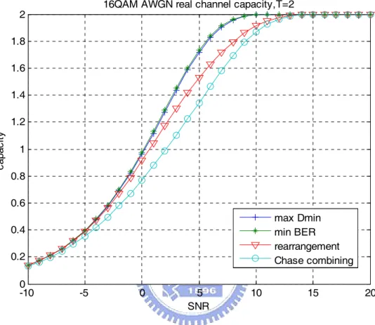
-10 -5 0 5 10 15 20 0 0.2 0.4 0.6 0.8 1 1.2 1.4 1.6 1.8 2 SNR ca pa ci ty

16QAM AWGN real channel capacity,T=2

max Dmin min BER rearrangement Chase combining

(33)

0 5 10 15 0 5 10 15 20 25 30 35 distance nu m ber o f s ign al pai rs distance distribution Gray,Gray rearrangement min BER max Dmin

Fig 4.2.2 distance distribution of different mapping schemes

Fig 4.2.1 compared the CM capacity for 16QAM in AWGN channels for some different mapping schemes in the literature and Fig 4.2.2 showed their corresponding distance distribution between signal pairs. Mapping designed for maximizing the minimum Euclidean distance (MDMIN) has high CM capacity since the nearest signal points have been pulled far apart. Similar behavior has been presented in the mapping designed for minimizing the BER upper bound (MBER) since the minimum Euclidean distance dominates the BER upper bound. The distance distribution has confirmed that they have largest minimum Euclidean distance. For constellation rearrangement, although the minimum Euclidean distance has not been enlarged compared to Chase combining, the number of signal pairs that have smallest distance have decreased. Therefore its CM capacity is larger than Chase combining.

The above argument applied to frequency none-selective fast fading channel as well. We assume that the receiver have perfect channel state information, the capacity

(34)

derivation is quite similar to AWGN channel.

(

)

(

)

(

) (

)

( ) (

)

(

)

(

)

_ 1, 2 1 2 1 2 1 2 1 2 1 2 1 2 1 2 1 2 1 2 1 1 1 1 ,..., ; , ,..., | , ,..., 1 ; , ,..., | , ,..., 1 { | , ,..., | , ,..., , , ,..., } 1 { | , ,..., , , ,..., } 1 { ... ... | , .. CM HARQ T T T t T T t t T T T t t T T t s j C I X X X Y Y Y H H H T I Y Y Y H H H T H H H H H Y Y Y H H H T H H Y Y Y H H H T n p y h T μ λ = = = − = − = − = L L L L L l

(

)

( ) ( )

(

)

(

)

(

)

(

)

(

)

(

)

1 1 1 1 1 1 2 1 1 1 1 1 . | , ... | , ... | , 1 log ... ... } (4.5) 2 | , ... | , t T t j t i s t T T j T T h h y y t t i T T i T T T n t t j T T j T p y h p h p h p y h p y h dy dy dh dh p y h p y h λ λ μ λ μ λ μ λ μ λ μ λ ∞ ∞ ∞ ∞ =−∞ =−∞ =−∞ =−∞ = ∈Λ = ∈Λ = ⋅ = = = =

∑ ∫

∫ ∫

∫

∑

l l l l l l l

4.3 Bit-Interleaved Coded Modulation Capacity

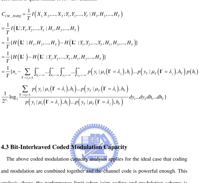
The above coded modulation capacity analysis applies for the ideal case that coding and modulation are combined together and the channel code is powerful enough. This analysis shows the performance limit when joint coding and modulation scheme is applied. However, when BICM scheme is adopted, which separates coding and modulation, the capacity will be different from the CM capacity. Similar to CM capacity, the BICM capacity is also affected by the choice of retransmission mappings. The derivation of BICM capacity with multiple transmissions is a direct extension of the BICM capacity with single transmission [3].

Fig 4.3.1 shows the equivalent parallel channel model for BICM under the assumption of ideal interleaving. S is the random variable whose outcome determines the switch position and is i.i.d. uniformly distributed over{1, 2,....,n . _s}

(35)

Encoder

Binary input channel 1

Binary input channel 2

Binary input channel ns S

Fig 4.3.1 Equivalent parallel channel model for BICM in the case of ideal interleaving

The BICM capacity with perfect CSI is given by (normalized with respect to T)

(

)

(

)

(

) (

)

(

)

( ) (

)

(

)

_ 1 2 1 2 1 2 1 2 1 1 2 1 2 1 2 1 1 2 1 2 1 1 ; , ,..., | , ,..., , 1 1 ; , ,..., | , ,..., , 1 { | , ,...., | , ,..., , , ,..., } 1 | , ,..., , , ,..., s s BICM HARQ s T T n t s k T T k s n t t k T k T T k t t k k T T k C n I c Y Y Y H H H S T n I L Y Y Y H H H s k T n H L H H H H L Y Y Y H H H T H L H L Y Y Y H H H T = = = = ⎛ ⎞ = _⎜ = _⎟ ⎝ ⎠ = − = −

∑

(

)

₍

(

)

₎

1 1 1 2 1 2 1 2 1 2 2 1 1 {0,1} ,..., ,..., 1 2 1 2 , ,..., , , ,..., 1 1 , , ,..., , , ,..., log ... , , ,..., , , ,..., s s t k T T n n T T t k T T t T k l b y y h h k T T p y y y h h h p l b y y y h h h dy dy T = = ∈ p l b y y y h h h ⎛ ⎞ ⎜ ⎟ = − = ⎜ ₌ ⎟ ⎝ ⎠

∑

∑ ∫ ∫

(4.6)

(36)

(

)

(

)

(

)

(

) (

)

1 2 1 1 2 1 1 2 1 1 2 1 2 1 2 1 2 where , , ,..., , ,..., , ,..., , ,..., , , , ,..., , ,..., , , ,..., | , ,..., , , ,..., | , ,..., t j t b j k t b j k t k T T t t T T j k t T T j t t t T T j T j j p l b y y y h h p y y y h h l b p y y y h h p y y y h h h p h h h p p y y y λ λ λ λ λ λ λ λ = ∈Λ = ∈Λ = ∈Λ = = = = = = = = = = =

∑

l l l l l l l l

(

)

(

)

(

)

(

) (

)

(

)

(

)

(

)

(

)

(

)

(

)

1 2 1 2 1 1 2 2 1 2 1 1 1 2 2 2 1 2 | , ,..., , , ,..., 1 | , | , ... | , , ,..., 2 1 | , | , ... | , , ,..., 2 t b j k s t b j k s t b j k t t T T j T j t t t j j T T j T n t t t j j T T T j T n h h h p h h h p p y h p y h p y h p h h h p y h p y h p y h p h h h λ λ λ λ λ λ λ λ μ λ μ λ μ λ = ∈Λ = ∈Λ = ∈Λ = = = = = = = = = =

∑

l l l l l l l l l l l (4.7)

(

)

(

)

(

) (

)

(

) (

)

(

)

(

)

1 2 1 2 1 1 2 1 1 2 1 2 1 1 2 2 1 2 , ,..., , , ,..., ,..., , , ,..., , ,..., | , ,..., , , ,..., | | , | , ... | , , ,..., t i t i t i T T t T T i t t t T T i T i i t t t t i i T T i T i p y y y h h h p y y h h h p y y h h h p h h h p p y h p y h p y h p h h h p λ λ λ λ λ λ λ λ λ λ λ = ∈Λ = ∈Λ = ∈Λ = = = = = = = = = = =

∑

l l l l l l l l l l l

(

) (

)

(

)

(

)

(

)

(

)

(

)

(

)

1 1 2 2 1 2 1 1 1 2 2 2 1 2 1 | , | , ... | , , ,..., 2 1 | , | , ... | , , ,..., (4.8) 2 s t i s t i t t t i i T T i T n t t t i i T T T i T n p y h p y h p y h p h h h p y h p y h p y h p h h h λ λ λ λ λ μ λ μ λ μ λ = ∈Λ = ∈Λ = = = = = = = =

∑

l l l l l l l l

(37)

(

)

(

)

(

)

(

)

(

)

(

)

(

)

(

)

(

)

(

)

(

)

1 2 1 1 1 1 1 2 1 {0,1} , ,..., ,..., 1 1 1 1 2 2 1 1 1 1 1 { (1 | , ... | , , ,..., 2 1 | , ... | , , ,..., 2 log | , ... | , s s t t b k T T j k s t i n t t j T T T j T n k l b y y y h h t t i T T T i T n t t j T T T j p y h p y h p h h h T p y h p y h p h h h p y h p y h p λ λ μ λ μ λ μ λ μ λ μ λ μ λ = = ∈ = ∈Λ = ∈Λ = − = = ⋅ = = = =

∑

∫

∑

l l l l l l l l

(

)

(

)

₍

₎

(

)

1 1 1 1 1 2 2 1 2 1 {0,1} ,..., ,..., 1 2 ... ,... } (4.9) 1 , ,..., 2 || || 1 1 { (1 exp ,..., 2 2 || exp log s t b j k s s t t b k T T j k T T T n t n T k k k j T n k l b y y h h k t k k k i dy dy dh dh h h h y h p h h T y h λ λ μ λ σ μ λ = ∈Λ = = ∈ = ∈Λ = ⎛ − = ⎞ ⎜ ⎟ = − _⎜− _⎟ ⋅ ⎝ ⎠ − = −

∑

∫ ∫

∑

l l l l

(

)

2 2 1 1 1 2 2 1 || 2 ... ,... } (4.10) || || exp 2 t i t b j k T k T T t T k k k j k dy dy dh dh y h λ λ σ μ λ σ = = ∈Λ = = ∈Λ ⎛ ⎞ ⎜ ⎟ ⎜ ⎟ ⎝ ⎠ ⎛ − = ⎞ ⎜− ⎟ ⎜ ⎟ ⎝ ⎠

∑

l l l

Different from the CM capacity which is only determined by the configuration of constellation points in the enlarged signal space, the BICM capacity also depends on the number of bit differences between symbols. The

term

( )

2 2 1 || || exp 2 b j k T k k k j k y h λ μ λ σ = ∈Λ ⎛ − ⎞ ⎜− ⎟ ⎜ ⎟ ⎝ ⎠

∑

, which is summed over those symbols whose

k-th bit is b, apparently depends strongly on the labeling on symbols. Since mappings designed to have large CM capacity often aim to enlarge the Euclidean distance between constellation points and ignore the effect of the number of bit differences between symbols, they do not necessary achieves high BICM capacity.

(38)

-15 -10 -5 0 5 10 15 20 0 0.2 0.4 0.6 0.8 1 1.2 1.4 1.6 1.8 2 E_s/N_o ca pa ci ty

16QAM AWGN real channel C_BICM T=2

rearrangement min BER max Dmin chase combining

Fig 4.3.2 BICM capacity of different mapping schemes

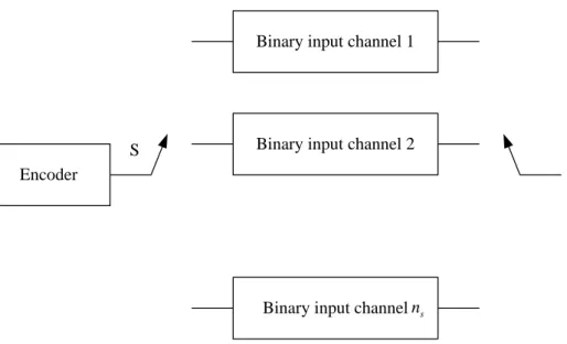
As shown in Fig 4.3.2, MBER and MDMIN have low BICM capacity at low SNR region, they outperform constellation rearrangement and Chase combining only at high SNR region. Constellation rearrangement, on the other hand, has higher BICM capacity than Chase Combining over the entire SNR range. Hence the behavior of BICM capacity is different from CM capacity and the design criterion for BICM systems should be different from CM systems.

在混合自動重傳機制中設計 位元交錯編碼調變及位元交錯編碼調變迭代解碼之 適應性多重傳輸位元映射規則

國 立 交 通 大 學

電信工程學系碩士班

碩 士 論 文