計數值兩階段相依製程的監控 - 政大學術集成

全文

(1)國立政治大學統計學系博士學位論文指導教授: 楊素芬博士計數值兩階段相依製程的監控 Monitoring a Two-Step Dependent Process 政治. 大. 立 Attribute Data With. ‧. ‧ 國. 學 er. io. sit. y. Nat. al. n. iv n Ch engchi U 研究生: 葉金田撰. 中華民國一百年七月.

(2) 謝辭從博士班入學口試到論文的完成, 終於告一段落, 在這段漫長的進修歲月中, 要感謝許多人對我的提攜與幫助. 首先要感謝我的指導老師楊素芬教授, 老師在學術上的認真態度讓人佩服, 不分寒暑假, 白天晚上都可以看到老師全力以赴的精神, 值得學習. 在研究過程中, 老師悉心指導, 啟發觀念, 很有耐心的引導學習, 使得本論文順利完成.. 立. 政治大. 感謝口試委員鄭惟孝教授, 曾勝滄教授, 葉小蓁教授與蔡紋琦教授,. ‧ 國. 學. 四位老師對論文仔細審閱並提出許多精闢的見解及意見, 使得本論. ‧. 文更臻完善. 在此致上無限的謝忱.. Nat. sit. al. er. io. 心.. y. 感謝何漢葳與許正宏兩位同學, 在這段期間的鼓勵與相處, 銘記在. n. iv n C heng 電腦部分感謝碩士班學生歐家玲, 林政憲, 余翊寧的協助, chi U. 使得計算. 順利完成最後要感謝我的太太, 她一直鼓勵我不斷的進修, 才有此成果. 本研究承蒙行政院國家科學委員會, 計畫編號 NSC 98-2118-M-004-005-MY2 補助, 謹此致謝.. 葉金田謹致.

(3) 計數值兩階段相依製程的監控. 學生: 葉金田. 指導教授: 楊素芬博士. 國立政治大學統計研究所博士班. 摘要. 政治大. 本論文探討計數值相依製程的管制方法, 內容如下:. 立. ‧ 國. 學. (1) 當製程資料來自二元二項分配, 以建構二元二項管制區域監控計數值相依製程.. ‧. (2) 當二元計數資料具中度以上相關, 建立選控圖以監控計數值相依. er. io. sit. y. Nat. 製程.. n. al (3) 若不合格品比率極為微小時, 以二個相依的二項管制圖監控計數 iv Ch. 值相依製程.. n engchi U. (4) 建立適應性管制圖以監控計數值相依製程. (5) 透過模擬與計算方式, 以平均連串長度及 AATS 來評估並比較以上所提方法的績效..

(4) Monitoring a Two-Step Dependent Process with Attribute Data Student: Jin-Tyan Yeh. Advisor: Dr. Su-Fen Yang. Department of Statistics National Chengchi University. Abstract The article considers the dependent process steps with attributes data. We explore the process monitoring from different viewpoints. (i) We consider the dependent binomial. 治政 data, then obtain the control limits on the Bivariate Binomial 大 control region, and the 立 effect of nonconforming rate on the control region is investigated; (ii) We consider the ‧ 國. 學. dependent Binomial control charts to detect nonconforming rates for dependent. ‧. binomial data; (iii) We use two cause selecting charts to monitor dependent process. sit. y. Nat. with attributes data, and then evaluate the performance of the proposed methods by. io. er. average run length; (iv) We investigate the variable sample size and sampling interval (VSSI) cause selecting charts for the dependent process steps with attributes data; (v). al. n. iv n C We study the design of VSSI EWMA selecting charts for controlling dependent h ecause ngchi U process steps with attributes data. We calculated the adjusted average time to signal. to measure the performance of the proposed charts. Numerical examples and simulation studies showed that the proposed charts have better performance than the tranditional Shewhart attributes control chart..

(5) Contents Chapter 1.. Introduction……………………………………………………………..1. Chapter 2.. Design of the Bivariate Binomial Control Region………………….......5. 2.1 Example………………………………………………………………………..7 2.2 The Effect of px and py on Control Region………………………………….....9 2.3 Numerical Example……………………………………………………………10 Chapter 3.. Design of Two Dependent Binomial Charts……………………………12. 3.1 Framework for Bivariat Binomial Charts……………………………………...12. 政治大 Using Cause Selecting Control Charts to Monitor Dependent Process 立. 3.2 Numerical Example…………………………………………………………....14 Chapter 4.. ‧ 國. 學. Steps with Attributes Data…………………………………………………………16 4.1 Construction of the Proposed Charts…………………………………………..16. ‧. 4.2 Numerical Example……………………………………………………………18 Cause Selecting Charts with Variable Sample Sizes and Sampling. sit. y. Nat. Chapter 5.. n. al. er. io. Intervals for two Dependent Process Steps with Attributes Data…………………20. i Un. v. 5.1 Design of VSSI Control Charts for Dependent Steps with Attributes Data…..20. Ch. engchi. 5.2 Performance Measurement for VSSI Z1 and Z2 Control Charts………………22 5.3 Performance Comparison between VSSI and FP schemes……………….…..25 Chapter 6.. Cause Selecting Charts with VSSI EWMA Control Charts for Two. Dependent Process Steps with Attributes Data…………………………………..31 6.1 The Distribution of the VSSI EWMA Control Charts for Dependent Steps with Attributes Dada ……………………………………………………………...31 6.2 Design the VSSI EWMA Control Charts for Dependent Steps with Attributes Data……………………………………………………………………. ……31 6.3 Performance Measurement for VSSI EWMA Control Charts……………….35. I.

(6) 6.4 Performance Comparison between VSSI EWMA and FP EWMA Charts….37 Chapter 7.. Performance Comparison of Bivariate Binomial Control and. Cause Selecting Charts…………………………………………………….41 7.1 In-control ARL Calculation…………………………………………………41 7.2 Out-of-control ARL Calculation…………………………………………….41 Chapter 8.. Conclusion……………………………………………………………45. References………………………………………………………………………….47 Appendix 1: The Calculation of Transition Probability for VSSI Control Charts…49. 治政 Appendix 2: The Fortran Program to Find the Upper 大Control Limit of Bivariate 立 Binomial Control Region for different n, p , p , ρ , and α =0.0027………55 x. y. ‧. ‧ 國. 學. n. er. io. sit. y. Nat. al. Ch. engchi. II. i Un. v.

(7) List of Tables Table 1. Control Limit on the UCL for (50, px, py, ρ ), α = 0.0027.........................7 Table 2. Control Limit on the UCL for (100, px, py, ρ), α = 0.0027…………………8 Table 3. Paint Defect Data, n = 100............................................................................10 Table 4. (L1, L2) for Different ρ, px, py , α = 0.0027..................................................14 Table 5. Paint Defect Data and Cause Selecting Values……………………………..19 Table 6. The Possible Process State for Using VSSI Charts…………………………25 Table 7. Specified VSSI AATS vs. FP AATS………………………………………...27. 治政 Table 8. AATS of Optimum and FS Charts under Various 大Combination of 立 Parameters……………………………………………………………………29 ‧ 國. 學. Table 9. The Possible Process States for Using VSSI EWMA Charts….…………..37. ‧. Table10. Specified AATS of the VSSI EWMA and FP EWMA Charts…………….39. sit. y. Nat. Table 11. ARL1 for Z1 and Z2 Chart, BB Control Region and Shewhart npx-npy. io. n. al. er. Chart…………………………………………………………………………………44. Ch. engchi. III. i Un. v.

(8) List of Figures Figure 1. Two-step Process for Attributes Data………………………………………6 Figure 2. BB Control Region for n = 25, px = 0.01, py = 0.03, ρ = 0.3, α = 0.0027 ………………………………………………………………………………………6 Figure 3. Bivariate Binomial Control Region for (50, px, py, ρ = 0.7), α = 0.0027. …………………………………………………………………………………........8 Figure 4. Bivariate Binomial Control Region for (100, px, py, ρ = 0.7), α = 0.0027.....9 Figure 5. Bivariate Binomial control region for (100, px, py, ρ), α=0.0027..................9 Figure 6. BB Control Region ((X, Y) ~ BB(n = 100, px = 0.0027, py = 0.088, ρ =. 政治大. 0.553)………………………………………………………………………….11. 立. Figure 7. npx and npy Charts………………………………………………………….14. ‧ 國. 學. Figure 8. Two-step Process with the occurrences of SCi…………………………….16 Figure 9. Z1 and Z2 charts……………………………………………………………19. ‧. Figure 10. The Structure of VSSI Z1 and Z2 Charts………………………………….20. y. Nat. sit. Figure 11. The Main Effects for Average of Saved AATS(%) under Various. n. al. er. io. Parameters……………………………………………………………………..28. i Un. v. Figure 12. The Main Effects for Average of Saved AATS(%) under Various. Ch. engchi. Parameters……………………………………………………………………..30 Figure 13. The Control Limits of VSSI EWMAz1 and EWMAz2 Control Charts…..32 Figure 14. The Main Effects for Average of Saved AATS(%) under Various Parameters…………………………………………………………………….40. IV.

(9) Chapter 1 Introduction Most of the products are always produced by several different process steps in these days. When the process steps are independent then a Shewhart control chart could be applied to monitor each individual step. However when many processes steps were dependent then the Shewhart charts are difficult to interpret the process state adequately. The multivariate control charts became a popular tool in quality control. Lowery and Montgomery (1995) reviewed Hotelling’s multivariate control chart, multivariate cumulative sum (MCUSUM) control chart, and multivariate exponentially weighed moving average (MEWMA) control chart. They also discussed. 治政 principal components and regression adjustment of variables 大 in multivariate quality 立 control. However, the multivariate control charts dealing with discrete data are ‧ 國. 學. lacking. Therefore, this research will focus on the dependent process with attributes. ‧. data.. sit. y. Nat. Let variable X i be the number of defects or nonconformities with respect to. n. al. pn ) be the vector of. er. io. quality characteristic i, i = 1, 2, • • •, n, and p  ( p1 , p2 ,. v. fraction nonconformities. However X i ' s are correlated. Hence, control chart for. Ch. engchi. i Un. multivariate attribute processes should be used. In an early paper, Patel (1973) proposed a Hotelling’s  2 chart to monitor the time-dependent observations from multivariate binomial or multivariate Poisson populations. Because of its complexity, the scheme has not been widely adopted in practice. Lu et al. (1998) proposed a multivariate np control chart (MNP) to deal with the multivariate attribute process. The weighed sum of nonconforming counts of each quality characteristic was defined as X statistics. Control limits of the Shewhart-type were derived based on this X statistics. The drawbacks of this work were the normality assumption and the lack of discussion about the performance of the MNP control chart. Niaki (2006) employed. 1.

(10) the concept of simultaneous confidence intervals to derive control limits for several correlated quality characteristics in a multi-attributes data. He took advantage of the bootstrap method in designing the control chart, compared its performance to other method. Niaki (2007) first proposed a new transformation technique to reduce the amount of skewness of distribution of the attributes data and then used a Hotelling’s control chart on the transformed data. Chiu and Kuo (2010) proposed to control the false alarm and to consider the correlation between attributes to monitor a bivariate binomial process. The drawback of these papers is that when an out-of-control signal is given, it is difficult to determine which component of the process is out-of-control.. the average run length (ARL) to evaluate its performance.. 學. ‧ 國. 治政 In this study, the attributes data come from a 大 bivariate binomial distribution. 立 Hence we construct a probability control region to monitor the attributes data and use ‧. When the true rate of nonconforming item is small, then the natural. sit. y. Nat. approximation to the bivariate binomial distribution suffers a series inaccuracy in the. io. dependent process steps with attribute data.. al. er. monitor process. Hence we propose two dependent binomial charts to monitor the. n. iv n C If the second step of a process then it is difficult to determine hiseout-of-control, ngchi U. the correct process state. Hence we applied an arcsine square root transformation. technique to reduce the amount of skewness of distribution of the attributes data so that the transformed data is approximately normal. We then use the cause selecting control chart to monitor the second process step. The cause selecting control chart is similar in concept to the regression control chart of Mandel (1969) in that a control chart is constructed for a variable only after the observation has been adjusted for the effect of some other random variable. Cause selecting control was first suggested by Zhang (1984). In the past ten years, many researchers have extended Zhang’s result. Wade and Woodall (1993) gave excellent review of the cause selecting control chart, 2.

(11) and discussed its relationship to the Hotelling’s T 2 control chart. In their opinion, the cause selecting control chart outperforms Hotelling’s T 2 control chart. Yang (1998) designed the X and cause selecting control charts to monitor the dependent process steps with minimal process cost using renewal equation approach. Yang (2005) addressed the control approach for dependent steps with over-adjusted means. So far, adaptive sampling procedures has been proven that it could detect small shift in process mean better than the fixed sample size and sample interval for one step process. Yang and Su (2006) proposed the variable sample size (VSS) cause selecting charts for controlling means in the dependent process steps. The X  e charts with variable sample. 立. 治政 sizes and sampling intervals 大. (VSSI) scheme were. proposed in Yang and Su (2007). We would propose to use VSSI control charts to. ‧ 國. 學. monitor the dependent process step with attributes data. The performance of the. sit. y. Nat. (AATS) derived by a Markov chain approach.. ‧. proposed VSSI control charts was measured by the adjusted average time to signal. io. er. The exponentially weighted moving average (EWMA) has been proven that it could detect small changes in the process mean and variance for one step process. For. n. al. two steps process, Yang and. iv n C Yu h (2009) proposed U e n g c h i VSI EWMA charts. to monitor. dependent process steps. We would propose the VSSI EWMA chart to monitor the dependent process step with attributes data. This paper is organized as follows. Chapter 2, we assume the attributes data come from a bivariate binomial distribution and construct the bivariate binomial control region for monitoring the dependent process steps. Chapter 3, when the nonconforming rate is small, two dependent binomial control charts were investigated. Chapter 4, we use cause selecting control charts to monitor the dependent 3.

(12) process steps.. The ARL is used to compare the performance with Shewhart control. charts. Chapter 5, VSSI control technique for two dependent process steps with attributes data was explored. The performance of the proposed VSSI control technique was measured by the adjusted average to signal (AATS) which is derived by a Markov chain approach. Chapter 6, the design of VSSI EWMA charts for two dependent process steps with attributes data was studied. The Markov chain approach is used to approximate AATA for shifts in the two –step process.. 治政 Chapter 7, performance comparison between the bivariate 大 binomial control region 立 and cause selecting charts is carried out. ‧ 國. 學. Chapter 8, we summarize the study and give some suggestions for future. ‧. io. sit. y. Nat. n. al. er. researches.. Ch. engchi. 4. i Un. v.

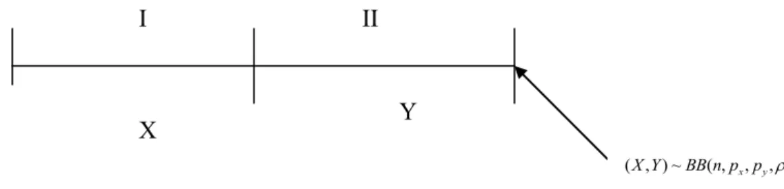
(13) Chapter 2 Design of the Bivariate Binomial Control Region Let X be the quality variable of interest on the first step, and Y the quality variable of interest on the second step. Since the two steps are dependent, hence Y is influenced by X. Here we assume that the paired data could only be collected at the end of the second step. A random sample of n units of a product was taken, and let X be the number of units of a specific part of the product that are nonconforming and Y be the number units of the product that are nonconforming. Y should be no less than X. The interested quality characteristics (X, Y) are assumed to follow a bivariate binomial distribution BB(n, px , p y ,  ) , where ρ is the correlation coefficient of X and. 學. ‧ 國. Y, and px , p y. 政治大 are fraction立 nonconforming for X and Y respectively. By Biswas and. Hwang (2002), the joint p.d.f of X and Y is given as:. ‧. n p( X  x, Y  y )    px x (1  px ) n  x f ( y | x),  x where. Nat. y.  x  n  x  i    { p y  w( p y  px )  w} i j ( i , j )S    x i *{1  p y  w( p y  px )} { p y  w( p y  px )} j. io. n. al. sit. . er. f ( y | x)  (1  w)  n. Ch. *{1  p y  w( p y  px )  w}n  x  j with S  {(i, j ) : i  j  y, i  0,1 w. k ,k  1 k. e n g cnh ix}. x, j  0,1. i Un. v. p y (1  p y ). (2.1). px (1  px ). Figure 1 shows the two-step process and the quality characteristics (X, Y) on the process.. 5.

(14) I. II. Y. X. ( X , Y ) ~ BB(n, px , p y ,  ). Fig. 1: two-step process for attributes data. From the assumption, Y should be no less then X, the conditional BB joint p.d.f is given by P(X=x, Y=y | X≦Y ) The control limits of the control region can be determined by taking the upper. 學. ‧ 國. 治政 percentage points of the exact probability distribution. 大 That is 立 P( (X Y, ) UCL X|  Y  ) where , X Y( UCL. ( x y, ). n x   px ( 0 ,x0).  px (n1 x f y ) x P( X |  Y) /  ( . ,. ‧. t h i s i m p l i es. , BB) n~ px (p y ,  ,. ) 1. ..........(2.2) .................... Nat. y. ). n. al. er. io. control region as follows:. sit. When n, px , py ,  ,  are given, we can construct the Bivariate Binomial (BB). Ch. engchi. i Un. v. Fig. 2. BB Control Region for n = 25, px = 0.01, py = 0.03, ρ = 0.3, α = 0.0027 6.

(15) In Fig. 2, A is the acceptance region, and R is the rejection region in the triangle area with specified n, pX, py, ρ = 0.3 and α = 0.0027. When the BB control region is determined, we can plot statistics (X, Y) on the BB control region and monitor the process. Appendix 2 is the Fortran program to find the upper control limit (UCLB) for different n, px, py, ρ , and α=0.0027 2.1 Example Table 1, 2 list critical points on the Upper Control Limit (UCL) for different n, pX, py, ρ , under α = 0.0027. 立. 政治大. ‧ 國. 學. Figure 3, 4 show the BB control region for different n, px , py ,  ,   0.0027 Table 1. Critical Points on the UCL for (50, px , py ,  )   0.0027 (0.01,0.03). ‧. (px, py). (0.01,0.05). al. n. iv n C h (3,6),(3,7),(4,6),(5,6),(6,6) engchi U (2,3),(2,4),…,(2,50), (2,6),(2,7),…(2,50) (3,4),(4,4). 0.5. (3,3) 0.7. sit. (2,7),(2,8),…,(2,50). er. (2,4),(2.5),…,(2,50),. io. 0.3. y. Nat. ρ. (0.03,0.05). (3,6),(4,5),(4,6),(5,5). (4,11),(4,12),… (4,50),(5,5),(5,6) (3,5),(3,6),…,(3,50) (4,4),(4,5). (1,3),(1,4),…,,(1,50), (2,5),(2,6),…,(2,50). (2,5),(2,6),…,(2.50). (2,2),(2,3). (3,3),(3,4),(3,5). (3,5),(4,5),(5,5). 7.

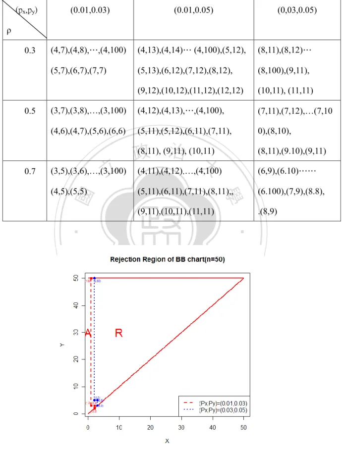
(16) Table 2. Critical Points on the UCL for (100, px , py ,  )   0.0027 (px,py). (0.01,0.03). (0.01,0.05). (0,03,0.05). (4,7),(4,8),…,(4,100). (4,13),(4,14)… (4,100),(5,12),. (8,11),(8,12)…. (5,7),(6,7),(7,7). (5,13),(6,12),(7,12),(8,12),. (8,100),(9,11),. (9,12),(10,12),(11,12),(12,12). (10,11), (11,11). (3,7),(3,8),…,(3,100). (4,12),(4,13),…,(4,100),. (7,11),(7,12),…(7,10. (4,6),(4,7),(5,6),(6,6). (5,11),(5,12),(6,11),(7,11),. 0),(8,10),. ρ. 立. (3,5),(3,6),…,(3,100). (4,11),(4,12).…,(4,100). (6,9),(6.10)……. (5,11),(6,11),(7,11),(8,11),,. (6.100),(7,9),(8.8),. (9,11),(10,11),(11,11). .(8,9). 學. (4,5),(5,5). (8,11),(9.10),(9,11). ‧ y. Nat. io. sit. 0.7. (8,11), (9,11), 治 (10,11) 政大. n. al. er. 0.5. ‧ 國. 0.3. Ch. engchi. i Un. v. Fig. 3. BB Control Region for (n=50, px, py, ρ = 0.7), α = 0.0027. 8.

(17) 立. 政治大. ‧ 國. 學. Fig. 4. BB Control Region for (n=100, px, py, ρ = 0.7), α = 0.0027. ‧. n. er. io. sit. y. Nat. al. Ch. engchi. i Un. v. Fig.5. BB Control Region for (n=100, Px = 0.03, Py = 0.05, ρ ), α = 0.0027 2.2 The Effect of px and py on Control Region From above figures, we can find for fix py that the area of acceptance region will 9.

(18) increase rightward and the area of rejection region will decrease gradually when the p x gets larger with ρ = 0.7.. As the value of p y gets bigger, the area of rejection region will decrease upward and the area of acceptance region will increase gradually for fix px 2.3. Numerical Example The paint defect data in Table 3 is taken from Mukhopadhyay (2008) but the sample size is revised to 100. This example is dealing with the proportion defective data with regard to two kinds of paint defects of a ceiling fan cover. Let X be the. 政治大. number of patty defect, and Y be the number of poor covering. The correlation. 立. coefficient of X and Y is 0.553.. 9. 13. 3. 3. 8. 14. 2. 11. y. 3. 10. 15. 2. sit. 7. 16. i Un. io. 3. 1. Nat. 2. Y. n. al. 4. 3. 5. 1. 6. 1. 6. 7. 2. 8. Sample number. X. Y 8. 7. er. ‧ 國. 1. X. ‧. Sample number. 學. Table 3. Paint Defect Data, n = 100. v. 2. 6. 5. 10. 18. 1. 7. 7. 19. 2. 8. 4. 8. 20. 10. 15. 9. 3. 8. 21. 3. 10. 10. 3. 14. 22. 2. 10. 11. 2. 15. 23. 3. 8. 12. 1. 5. 24. 2. 10. Ch 3. e n g c17h i. 10.

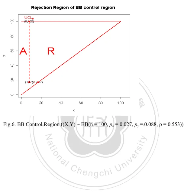
(19) Figure 6 reveals (X, Y)’s are all in acceptance region of the BB control region. It indicates the two process steps are in control.. 立. 政治大. ‧. ‧ 國. 學. Fig.6. BB Control Region ((X,Y) ~ BB(n = 100, px = 0.027, py = 0.088, ρ = 0.553)). n. er. io. sit. y. Nat. al. Ch. engchi. 11. i Un. v.

(20) Chapter 3 Design of Two Dependent Binomial Charts The drawback of the BB control region is that it is not easy to distinguish which quality variable is out of control or which process step is out of control. To solve this problem, in this section, we construct two dependent Binomial control charts, say np X and and npY charts. The np X chart is constructed to monitor the number of. nonconforming for X and npY chart is constructed to monitor the number of nonconforming for Y. The two charts are dependent since X and Y are dependent. 3.1 Framework for Two Dependent Binomial Charts. 政治大. Since X ~ B(n, p X ) and Y ~ B(n, pY ) s.t. X≦Y but with correlation coefficient . 立. (3.1). y. UCL2  npY  L2 npY (1  pY ). and. LCL2  npY  L2 npY (1  pY ). io. sit. Nat. LCL1  npX  L1 npX (1  p X ). and. (3.2). er. UCL1  npX  L1 npX (1  p X ). ‧. ‧ 國. given below.. 學. for in-control process steps. Hence, the control limits of the np X and npY charts are. To let the two charts with in-control ARL=370, the L1 and L2 are chosen to minimize. al. n. iv n C the absolute deviation of the in-control run length (ARL) from the nominal h e naverage gchi U value instead of the factor of control limits=3 of a traditional Shewhart np chart.. To find reasonable L1 and L2 with fairly allocated marginal type I error probability of the two charts, it is important to keep both charts with approximate power to detect process shifts. Given a specified type I error probability α, Jiang et. (2002) has proposed a heuristic algorithm to solve this problem. The optimal problem can be modeled as below:. 12.

(21) min ( L1 , L2 ). 1 npx  L1 npx (1  px )  X  npx  L1 npx (1  px ),    np y  L1 np y (1  p y )  X  np y  L1 np y (1  p y ) X  Y  P        1. s.t. L2  min. P{npx  L1 npx (1  px )  X  npx  L1 npx (1  px }. . 1 (1   ). (3.3). . 1. L2. 政治大. P{np y  L2 np y (1  p y )  Y  np y  L2 np y (1  p y }. 立. (3.4). ‧ 國. 學. Note that equation (3.3) seeks factors L1 and L2 with minimum deviations to the. sit. y. Nat. have approximately the same power in detecting shifts.. ‧. reciprocal of the nominal tail areas, and equation (3.4) ensures both control charts. io. er. The algorithm in equation (3.3) and (3.4) can be easily implemented by a grid search. Table 4 is (L1, L2) for Bivariate Binomial Control Charts with different px, py, and ρ. al. n. iv n C Once the control limits for thehtwo control charts e n g c h i U were obtained, the number of. nonconforming for each attribute was plotted on the control chart for a specified overall α level. A signal by any one of the two control charts indicated that the process might be out-of-control.. 13.

(22) Table 4. (L1, L2) for Different ρ, pX, pY under α = 0.0027 (0.01, 0.03). (0.01,0.05). (0.03, 0.05). 0.3. (3.01, 3.47). (3.01, 3.58). (3.47, 3.14). 0.5. (3.12, 3.51). (3.12, 3.60). (3.51, 3.21). 0.7. (3.23, 3.62). (3.23, 3.67). (3.62, 3.32). (px,py) ρ. From Table 4, we found that L1 and L2 increase, but the width of the conditional. 政治大 Bivariate Binomial Control Chart decreases when ρ increases. 立 3.2 Numerical Example. ‧ 國. 學. To illustrate the use of the proposed construction and the use of the proposed. ‧. control charts for a given α = 0.0027, we use the paint data in Table 3. At α = 0.0027,. sit. y. Nat. the constant L1 and L2 are 3.12 and 3.23 respectively. With L1 and L2, we could. io. n. al. er. construct the control charts for two quality characteristics as in Fig.7.. np chart for X. 1. 10. Ch. 20. 6. 4 __ NP=2.67. 3. 5. 7. 9. 11 13 15 Sample. 17. 19. 21. __ NP=8.75. 5. -3.1SL=0 1. +3.1SL=17.57. 10. 2. 0. v. np chart for Y. 15. +3.1SL=7.69 Sample Count. Sample Count. 8. engchi. i Un. 0. -3.1SL=0 1. 23. 3. 5. 7. 9. 11 13 15 Sample. 17. 19. 21. 23. Fig.7. npX and npY Charts From Fig.7 there is a signal on sample #20 for npX chart, it means the first process step should be stopped and investigated for any possible assignable causes. The result is different from that of the BB chart. 14.

(23) The drawback of the npX and npY charts is they cannot distinguish if the second process step is in-control or not. For example, if a signal comes from the npY chart then the source may be from out-of control step 1 and /or step 2.. 立. 政治大. ‧. ‧ 國. 學. n. er. io. sit. y. Nat. al. Ch. engchi. 15. i Un. v.

(24) Chapter 4 Using Z1 and Z 2 Cause Selecting Charts to Monitor Dependent Process Steps with Attributes Data 4.1 Construction of the Proposed Z1 and Z 2 Charts In this section, the Z1 and Z 2 Cause Selecting Charts are proposed to monitor the same two dependent steps with attributes data. The quality variables on the two dependent process steps and data collection are illustrated in Fig. 8. Assume there are two special causes, SC1 and SC2, that may affect the quality variable and that SC1 only occurs in the first step, while SC2 only occurs in the. 治政 second step. In addition, we assume that if at least one大 special cause occurs in one of 立 the process steps, the process is out- of-control. Also, let T be the time until the SCi. ‧ 國. 學. occurrence of SCi, and it follows an exponential distribution with parameter λi. i.e. i 0 , , 1 , 2. (4.1). 1 is the mean time of TSCi that the process step i remains in a state of i. sit. n. al. er. io. statistical control.. y. Nat. where. t ),. ‧. f (t ) i e x p(i t. SC1 I. Ch. i Un. v. i e n g c h SC2 II. sampling X. Y. (x,y). Fig.8: Two-step process with the occurrence of SCi. . The distributions of X and Y is not symmetric, to solve the asymmetric problem, Ryan (1989) proposed an arcsine square root approach of normalized transformation. That 16.

(25) is X ~ N (sin 1 n. X*= sin 1. px ,. 1 Y ) , Y *  sin 1 ~ N (sin 1 4n n. py ,. 1 ) . Since the 4n. studied two process steps are dependent and the second step is influenced by the first step, following Wade and Wood (1993), the relation of Y* and X* may be expressed. Y *  f ( X *) . . ,. ~N (20 ,. (4.2). ). In order to exclude the effect of the first step while monitoring the second step, we let. e  Y*  ˆY* ~ N (0 2,. (4.3). ). where Yˆ * is fitted value of f(X*). X * ~ N (sin 1. px ,. 學. ‧ 國. 治政 To control the two dependent process steps effectively, 大 the X* chart and e chart 立 (cause selecting control chart) are used. When both steps are in-control, 1 ) 4n. (4.4). e ~ N (0,  ). e. y. ~ N (0,1). al. n. . io. Z2 . px ) 4n ~ N (0,1). sit. Z1  ( X *  sin 1. er. Nat. This implies. ‧. 2. The control limits of Z1 and. C Z h 2. i Un. engchi. charts are. UCLZ1  K Z 1. UCLZ 2 K Z. CLZ1  0. CLZ2  0. LCLZ1   K Z1. LCLZ2   K Z2. (4.5). v. 2. (4.6). We would use Z1 chart to monitor the first process step, and Z 2 chart to monitor the second process step. While SC1 may only occur in the first step, SC2 may only occur in the second step. The out-of-control distribution of X and e are as follows.. 17.

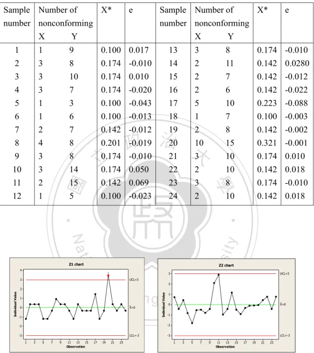
(26) X ~ B(n, 1 px ) 1  1. (4.7). e ~ N ( 2 ,  2 )  2  0 This implies. X *  sin 1. X 1 ~ N (sin 1 1 px , ) n 4n px ) 4n ~ N ((sin 1 1 px  sin 1. Z1  ( X *  sin 1 Z2 . e. . px ) 4n ,1). ~ N ( 2 ,1). (4.8). 政治大 Taking the same example data in Table 3. Let X be the number of patty defect, 立. 4.2. Numerical Example. take. the. arcsine. square. root. transformation,. that. is. X Y , Y *  sin 1 . Then, find the relationship of Y* and X*. Scatter plot n n. sit. y. Nat. X *  sin 1. first. ‧. We. ‧ 國. 0.553.. 學. and Y be the number of poor covering. The correlation coefficient of X and Y is. n. al. er. io. indicates that the relationship of Y * and X * is linear. Using the least square error. i Un. method to find their relationship, the regression model is. Ch. Yˆ*  0.0643  0.874 X *. engchi. v. The residual is e = Y* – (0.0643 + 0.874X*) The in-control distribution of e is N (0, (0.002) 2 ) . Now using X* and e values (Table5) to construct the Z1 and Z2 charts (see Figure 9). Figure 9 indicated there is a signal (on the sample #20) on the Z1 chart, but no signal on Z2 chart. Based on this finding, the first process step should be stopped to investigate if there were any possible assignable causes. The result is same as the npX and npY Charts. 18.

(27) Table 5. Paint Defect Data and Cause Selecting Values Sample Number of X* number nonconforming X Y. e. Sample Number of X* number nonconforming X Y. e. 1 2 3. 1 3 3. 9 8 10. 0.100 0.017 0.174 -0.010 0.174 0.010. 13 14 15. 3 2 2. 8 11 7. 0.174 -0.010 0.142 0.0280 0.142 -0.012. 4 5 6 7 8. 3 1 1 2 4. 7 3 6 7 8. 0.174 0.100 0.100 0.142 0.201. 16 17 18 19 20. 2 5 1 2 10. 6 10 7 8 15. 0.142 0.223 0.100 0.142 0.321. -0.022 -0.088 -0.003 -0.002 -0.001. 9 10 11 12. 3 3 2 1. 8 14 15 5. 3 2. 10 10 8 10. 0.174 0.142 0.174 0.142. 0.010 0.018 -0.010 0.018. -0.020 -0.043 -0.013 -0.012 -0.019. 政治大 -0.010 21 3 立0.174 0.174 0.050 22 2. ‧. ‧ 國. 23 24. 學. 0.142 0.069 0.100 -0.023. io. sit. y. Nat Z1 chart. 2 1. er. al. n. 3. Individual Value. Z2 chart. 1. 3. UCL=3. Ch. n engchi U 2. Individual Value. 4. _ X=0. 0 -1. iv. UCL=3. 1. _ X=0. 0. -1 -2. -2 -3. -3. LCL=-3 1. 3. 5. 7. 9. 11 13 15 Observation. 17. 19. 21. 23. LCL=-3 1. 3. 5. Fig.9. Z1 and Z2 Charts. 19. 7. 9. 11 13 15 Observation. 17. 19. 21. 23.

(28) Chapter 5 Cause Selecting Charts with Variable Sample Sizes and Sampling Intervals for Two Dependent Process Steps 5.1 Design VSSI Control Charts for Dependent Steps with Attributes Data In this section, we will explore the adaptive control technique to monitor the dependent process step with attributes data. The variable sampling size and sample interval (VSSI) have been proved that it can detect small and moderate shifts in process mean and variance better than the fixed sample interval. The VSSI means that when there is some indication that a process parameter may be changed, the next. 治政 sampling interval should be shorter and the sample size 大should be larger. On the other 立 hand, if there were no indication, the next sampling interval should be longer and the ‧ 國. 學. sample size should be smaller.. to monitor the first step process, and Z 2. ‧. Based on the section 4.1, we use Z1. sit. y. Nat. chart to monitor the second step process. When both step are in-control or. n. al. er. io. out-of-control, the distributions of X* and e are the same as chapter 4.1.. i Un. v. The structure of the VSSI Z1 and Z 2 control charts under in control condition is as follows. Ch. engchi. UCLz1=K1. UCLZ2=K2. UWLZ1=W1. UWLZ2=W2. CLZ1=0. ClZ2=0. LWLZ1=-W1. LWLZ2=-W2. LCLZ1=-K1. LCLZ2=-K2. Fig.10. The Structure of VSSI Z1 and Z 2 Charts. 20.

(29) Here we divided the VSSI Z1 and Z 2 control charts into three regions. Let the interval (W1,-W1) be the central region (CR1) and interval (K1, W1)∪(-K1, -W1) be the warning region (WR1) of Z1 chart. Let the interval (-W2, W2) be the central region (CR2) and interval (-K2, -W2)∪(W2, K2) be the warning region (WR2) of Z 2 chart. Since using the two VSSI Z1 and Z 2 control charts, three variable sample interval hq, and three variable sizes nq, q=1,2,3 are adopted, 0  h3  h2  h1   , 0  n1  n2  n3   , The choice of (hq, nq) for the next sample depends on the. 政治大. position of the statistic Z1 and Z 2 . If all the sample points for Z1 and Z 2 fall. 立. within the central regions then the next sample should be small (n1) and sampling. ‧ 國. 學. interval should be long (h1). If one of the sample points for Z1 and Z 2 fall within. ‧. the warning region then the next sample should be medium (n2) and sampling interval. sit. y. Nat. should be medium (h2). If all the sample points for Z1 and Z 2 fall within the. al. n. should be short (h3).. er. io. warning regions then the next sample should be large (n3) and sampling interval. Ch. engchi. i Un. v. To compare the performance of VSSI and FP charts, we should use the same average sample size and average sampling interval under the in-control period. h1 p0 1 h 2 p 02 h 2p 0 3 h p3  0 4 h. 0. n1 p0 1 n 2 p 02 n 2p 0 3 n p3  0 4 n. 0. ( 5 . 1) (5.2). where p01  p ( Z1  W1 | Z1  K1 ) p ( Z 2  W2 | Z 2  K 2 ) p02  p ( Z1  W1 | Z1  K1 ) p (W2  Z 2  K 2 | Z 2  K 2 ) p03  p ( Z 2  W2 | Z 2  K 2 ) p (W1  Z1  K1 | Z1  K1 ). (5.3). p04  1  p01  p02  p03. According to Costa (1998), to facilitate the computation of the performance 21.

(30) measure, during the in-control period the conditional probability of a sample point falling in the central region (or the warning region), given that it falls in the control region, is the same for both the Z1 and Z 2 chart. That is, p( Z1  W1 | Z1 . K1) . p( Z2 . Z2 . W 2|. K )2 . p. (5.4). 0. The procedure to derive the warning limits is as follows: Step 1. From equations (5.3) and (5.4), we obtained. p01  p02 , p02  (1  p0 ) p0. p03  p0 (1  p0 ). p04  (1  p0 )2. (5.5). Step 2. Put the results of Step1 in equation (5.1), we can obtain 2 (n3  n2 ). 立. 2. 2 3. 1. 2. 3. n) 3( n0. 2 (n1  2n2  n3 ). ). (5.6). 學. ‧ 國. p0 . 政治大 ( 2n(  n ) 4n ( n2  n. Step 3. Specify n0, n1, n2, h3, then we can get w1, w2 and h1 below: p0 (2( K1 )  1)  1) ) =W 2 h0  (2 p0  2 p0 2 )h2  (1  p0 ) 2 h3 h1  p0 2. ‧. W1  W2   1 (. n. er. io. sit. y. Nat. al. (5.7). Ch. i Un. v. 5.2 Performance Measurement for VSSI Z1 and Z 2 Control Charts. engchi. To compare the performance of VSSI and FP charts, the adjusted average time to signal (AATS) is used as performance criteria. The smaller AATS is, the better performance of the proposed charts. The AATS is the mean time the process remains out-of-control. Since TSCI ~ exp(i ) , i = 1, 2, thus T(1) ~ exp(1  2 ) , where. T(1)  min(TSC1 , TSC 2 ) is the occurrence time until the first special cause occurs. Hence AATS  ATC . 1 1  2. (5.8). The average time of the cycle (ATC) is the average time from the process starts until the first true signal occurs. The memory-less property of the exponential distribution 22.

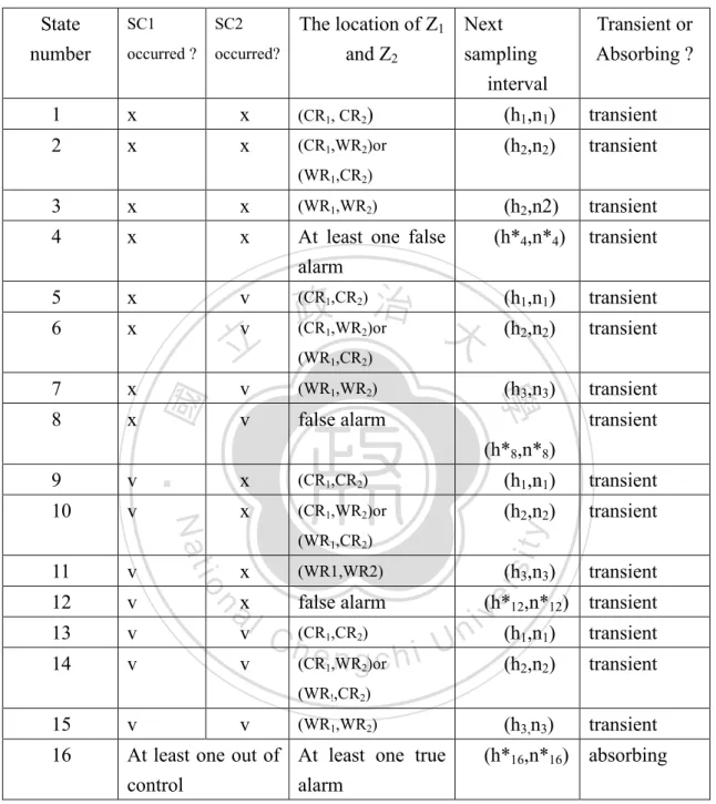
(31) allows the computation of the ATC through a Markov chain approach. We used the Markov chain approach to derive the AATS, and all possible process states for using VSSI Z1 and Z 2 charts must be defined. After each sampling, one of these possible states is reached according to the occurrence of the special cause and the location of the sample points in Z1 and Z 2 charts. The control charts produce a signal when at least one of the sample points falls outside the control limits. Table 6 showed the 16 possible process states, which can be classified into transient and absorbing states based on Markov property. State 1 to State 15 are. 政治大. transient states since they may transit to other states, while State 16 is an absorbing. 立. state since it cannot transit to any other state.. ‧ 國. 學. After defining all possible states at each end of the sampling time, the transition probability from State i to State j with variable sampling intervals and sample sizes. ‧. (hq , nq ), Pi , j (hq , nq ) is calculated.. er. io. sit. y. Nat. For example,. al. n. iv n C  W | Zh~ N ( n  ,1)) P (TU  h ) P (T engchi. P1,5 (h1 , n1 )  P ( Z1  W ) P ( Z 2. 2. 1. 2. SC1. 1. SC 2.  h1 ).  (2(W )  1)(( (W   2 n1 )   (W   2 n1 )) exp(1 h1 )(1  2 h1 ) P3,12 (h3 , n3 )  ( (( K  sin 1 1 px )  sin 1 sin 1. px ) 4n3  (( K  sin 1 1 px ) . (5.9). px ) 4n3 )2(1  ( K )(1  exp(1 h3 ) exp(2 h3 ). The transition probability from States i to j can be expressed by a square matrix. Q P 0. A , where Q1515 is the transition probability matrix with each element I . Expressing the transition probability from State i to transient to State j. Pi , j (hq , nq ), i  1, 15, j  1, 15, q  1, 2,3. 23. A  ( p1 , 1 ,6 p. ,. 2 ,1 6. p. ).  1 5 ,1 6. 1 1 5.

(32) where pi ,16 is the transient probability from State i to State 16. 0115 is the vector with all elements being zero and I11 is the probability 1 for staying at the absorbing State 16. From the elementary properties of Markov chains (Cinlar, 1975), the ATC is as ATC   ( I  Q ) 1 t. (5.10). Where.    ( 1 , 2 , 3 , 0,. 0).  ( p01 , p02  p03 , p04 , 0,. 0) is a (1X15) vector with the starting probability. for transient state i, i=1,.......15,. 政治大 interval time for transient state i, i=1,.....15, 立. t   (h1 ,h 2 ,h 3 ,h *4 ,h1 ,h 2 h 3 ,h*8 ,h1 ,h 2 ,h 3 ,h *12 ,h1 ,h 2 ,h 3 ) is a (15X1) vector of sampling. ‧ 國. 學. h*4 is the average time of sample interval for state 1-3, h*8 is the average time of sample interval for state 5-7,. ‧. h*12 is the average time of sample interval for state 9-11.. n. er. io. sit. y. Nat. al. Ch. engchi. 24. i Un. v.

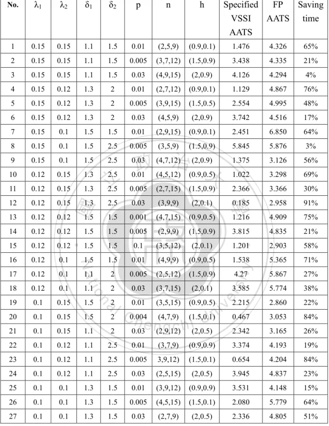
(33) Table 6. The Possible Process States for Using VSSI Z1 and Z 2 Charts State number. The location of Z1 Next occurred ? occurred? and Z2 sampling interval SC1. SC2. Transient or Absorbing ?. 1. x. x. (CR1, CR2). (h1,n1). transient. 2. x. x. (CR1,WR2)or. (h2,n2). transient. (h2,n2). transient. (h*4,n*4). transient. (h1,n1). transient. (h2,n2). transient. (h3,n3). transient. (WR1,CR2). 3. x. x. (WR1,WR2). 4. x. x. At least one false alarm. 5. x. v. 6. x. v. (CR ,CR ) 治政 (CR ,WR )or 大. v. 12. v. 13 14. false alarm. transient. x. (CR1,CR2). (h1,n1). transient. x. (CR1,WR2)or. (h2,n2). transient. (WR1,CR2). x. (WR1,WR2). false alarm. v. axl. v. v. n. v. io. 11. v. v. C h(CR ,CR ) e ,WR n g)orc h i U (CR 1 1. 2. 2. y. 10. (WR1,WR2). ‧. v. v. (h*8,n*8). Nat. 9. (WR1,CR2). sit. x. 2. (h3,n3). er. 8. ‧ 國. x. 1. 2. 學. 7. 立. 1. transient. (h*12,n*12) transient. v n i (h1,n1). transient. (h2,n2). transient. (h3,n3). transient. (WR!,CR2). 15. v. v. 16. At least one out of At least one true control alarm. (WR1,WR2). (h*16,n*16) absorbing. Note n*i= the average sample size for state i, i=4, 8, 12, 16.. 5.3 Performance Comparison between VSSI and FP Scheme Table 7 provide the AATS of the VSSI and FP schemes, which were obtained under various combinations of parameters based on orthogonal (L27) table. The specified parameters are λ1 = (0.15,0.12,0.1), λ2 = (0.15,0.12,0.1). δ1 = (1.1,1.3,1.5), δ2 = (1.5,2.3), (h2,h3) = (0.9,1.5,2), (0.1,0.5,0.9), (n1,n2,n3) = (2,3,4), (5,7,9), (9,13,15) 25.

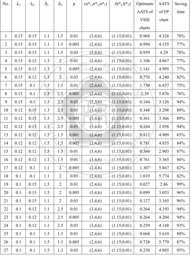
(34) We found that the VSSI control charts saved detection time from 3% to 91% compared to the FP control charts. We also created main effects plots for the saved AATS under various parameters. Fig.11 indicate that parameters δ1, n1, h2, h3, are significant. As δ1 or n1 increases, AATS increases. As h2 or h3 increases, AATS decreases. Sometimes the adopted specified VSSI may not good to have better AATS, the optimal VSSI’s of the proposed charts are thus suggested. The optimal VSSI of the proposed charts are determined using optimization technique to minimize AATS. The mathematical expression for the optimum VSSI control charts is. 0.01  h3  1  h2  h1  3. 1  n1  3  n2  n3  10. 學. ‧ 國. 治政 Objective function: Minimize AATS 大立 Subject to:. (5.11). ‧. Given ( , 1 , 2 , 1 ,  2 , K1 , K 2 ). sit. y. Nat. The optimum VSSI and AATS under various combinations of parameters are. io. er. illustrated in Table 9. We found that the optimum VSSI control charts save detection time from 75% to 99% compared to the FP control charts, and the optimum VSSI. al. n. iv n C better than FP control charts h ethe ngchi U. control charts also work sampling intervals.. with specific variable. To examine the effects of various parameters on the optimum VSSI and AATS, the main effect plots show the significant parameters are λ1, λ2, δ1 and δ2 (Fig. 12). As λ2, δ1 or δ2 increases, AATS increases. As λ1 increases, AATS decreases.. 26.

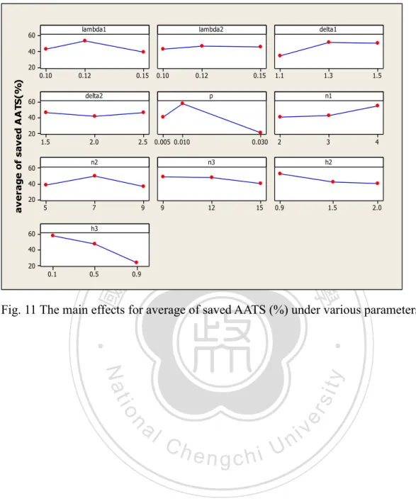
(35) Table 7. Specified VSSI AATS vs. FP AATS λ1. λ2. δ1. δ2. p. n. h. 1. 0.15. 0.15. 1.1. 1.5. 0.01. (2,5,9). (0.9,0.1). 1.476. 4.326. 65%. 2. 0.15. 0.15. 1.1. 1.5. 0.005. (3,7,12). (1.5,0.9). 3.438. 4.335. 21%. 3. 0.15. 0.15. 1.1. 1.5. 0.03. (4,9,15). (2,0.9). 4.126. 4.294. 4%. 4. 0.15. 0.12. 1.3. 2. 0.01. (2,7,12). (0.9,0.1). 1.129. 4.867. 76%. 5. 0.15. 0.12. 1.3. 2. 0.005. (3,9,15). (1.5,0.5). 2.554. 4.995. 48%. 6. 0.15. 0.12. 1.3. 2. 0.03. (4,5,9). (2,0.9). 3.742. 4.516. 17%. 7. 0.15. 0.1. 1.5. 1.5. 0.01. (2,9,15). (0.9,0.1). 2.451. 6.850. 64%. 8. 0.15. 0.1. 1.5. 2.5. 0.005. (3,5,9). (1.5,0.9). 5.845. 5.876. 3%. 9. 0.15. 0.1. 1.5. 2.5. 0.03. 1.375. 3.126. 56%. 10. 0.12. 0.15. 1.3. 2.5. 3.298. 69%. 11. 0.12. 0.15. 1.3. 立 2.5. 1.022. 0.005. (2,7,15). (1.5,0.9). 2.366. 3.366. 30%. 12. 0.12. 0.15. 1.3. 2.5. 0.03. (3,9,9). (2,0.1). 0.185. 2.958. 91%. 13. 0.12. 0.12. 1.5. 1.5. 0.001. (4,7,15). (0.9,0.5). 1.216. 4.909. 75%. 14. 0.12. 0.12. 1.5. 1.5. 0.005. (2,9,9). (1.5,0.9). 3.815. 4.835. 21%. 15. 0.12. 0.12. 1.5. 1.5. 0.1. (3,5,12). (2,0.1). 1.201. 2.903. 58%. 16. 0.12. 0.1. 1.5. 1.5. 0.01. (4,9,9). (0.9,0.5). 1.538. 5.365. 71%. 17. 0.12. 0.1. 1.1. 2. 0.005. (2,5,12). (1.5,0.9). 4.27. 5.867. 27%. 18. 0.12. 0.1. 1.1. 2. 0.03. (3,7,15). (2,0.1). 3.585. 5.774. 38%. 19. 0.1. 0.15. 1.5. 22%. 0.1. 0.15. 1.5. 3.053. 84%. 21. 0.1. 0.15. 1.1. 2. v 2.215 i C0.004 (1.5,0.1)n 0.467 U h e n(4,7,9) i h g c (2,0.5) 2.342 0.03 (2,9,12). 2.860. 20. a2l. 3.165. 26%. 22. 0.1. 0.12. 1.1. 2.5. 0.01. (3,7,9). (0.9,0.9). 3.374. 4.193. 19%. 23. 0.1. 0.12. 1.1. 2.5. 0.005. 3,9,12). (1.5,0.1). 0.654. 4.204. 84%. 24. 0.1. 0.12. 1.1. 2.5. 0.03. (2,5,15). (2,0.5). 3.945. 4.837. 23%. 25. 0.1. 0.1. 1.3. 1.5. 0.01. (3,9,12). (0.9,0.9). 3.531. 4.148. 15%. 26. 0.1. 0.1. 1.3. 1.5. 0.005. (4,5,15). (1.5,0.1). 2.080. 5.779. 64%. 27. 0.1. 0.1. 1.3. 1.5. 0.03. (2,7,9). (2,0.5). 2.336. 4.805. 51%. (4,7,12) 治 (2,0.9) 政大 0.01 (4,5,12) (0.9,0.5). n. (3,5,15). 27. (0.9,0.5). y. sit er. io. 0.01. ‧. Nat. 2. Specified FP Saving VSSI AATS time AATS. 學. ‧ 國. No..

(36) lambda1. 60. lambda2. delta1. 40 20. average of saved AATS(%). 0.10. 0.12. 0.15. 0.10. 0.12. delta2. 60. 0.15. 1.1. 1.3. p. 1.5. n1. 40 20 1.5. 2.0. 2.5. 0.005 0.010. n2. 60. 0.030. 2. 3. n3. 4. h2. 40 20 5. 7. 9. h3. 60 40. 立. 20 0.5. 12. 15. 0.9. 1.5. 2.0. 政治大. 0.9. 學. ‧ 國. 0.1. 9. Fig. 11 The main effects for average of saved AATS (%) under various parameters. ‧. n. er. io. sit. y. Nat. al. Ch. engchi. 28. i Un. v.

(37) Table 8. AATS of Optimum VSSI and FP Charts under Various Combination of Parameters No.. λ1. λ2. δ1. δ2. p. (n*1,n*2,n*3). (h*2,h*3). Optimum. AATS. Saving. AATS of. of FP. time. VSSI. chart. 1. 0.15. 0.15. 1.1. 1.5. 0.01. (3,4,6). (1.15,0.01). 0.968. 4.326. 78%. 2. 0.15. 0.15. 1.1. 1.5. 0.005. (2,4,6). (1.15,0.01). 0.994. 4.335. 77%. 3. 0.15. 0.15. 1.1. 1.5. 0.03. (3,4,6). (1.15,0.01). 0.959. 4.29. 78%. 4. 0.15. 0.12. 1.3. 2. 0.01. (3,4,6). (1.15,0.01). 1.106. 4.867. 77%. 5. 0.15. 0.12. 1.3. 2. 0.005. 1.141. 4.995. 77%. 6. 0.15. 0.12. 1.3. 7. 0.15. 0.1. 1.5. 8. 0.15. 0.1. 9. 0.15. 0.1. 10. 0.12. 0.15. 11. 0.12. 0.15. ‧ 國. charts. 12. 0.12. 0.15. 1.3. 13. 0.12. 0.12. 1.5. 14. 0.12. 0.12. 1.5. 15. 0.12. 0.12. 1.5. 16. 0.12. 0.12. 1.1. 1.5. 17. 0.12. 0.1. 1.1. 2. 0.005. 18. 0.1. 0.1. 1.1. 2. 19. 0.1. 0.15. 1.5. 20. 0.1. 0.15. 21. 0.1. 22. 0.03 立 1.5 0.01. (2,4,6). (1.15,0.01). 0.776. 4.240. 82%. (2,4,6). (1.15,0.01). 1.739. 6.857. 75%. (2,4,6). (1.15,0.01). 1.39. 5.876. 76%. 1.5. 2.5. 0.03. (2,3,6). (1.15,0.01). 0.184. 3.126. 94%. 1.3. 2.5. 0.01. (3,4,6). (1.15,0.01). 0.348. 3.298. 89%. 1.3. 2.5. 0.005. (3,4,6). (1.15,0.01). 0.361. 3.366. 89%. 2.5. 0.03. (3,4,6). (1.15,0.01). 0.184. y. 2.958. 94%. 1.5. 0.001. (2,4,6). (1.15,0.01). 0.812. 4.909. 83%. 0.005. (2,4,6). (1.15,0.01). 0.781. 4.835. 84%. (3,4,6). (1.15,0.01). 0.364. 2.903. 87%. 0.761. 5.365. 86%. io. 1.5. n. a 1.5 l. 0.01. C 0.01h. er. 0.005. ‧. 學. 2.5. Nat. 1.5. sit. 2. 政 (2,4,6)治 (1.15,0.01) 大. iv n U e n(3,4,6) g c h i(1.15,0.01) (2,4,6). (1.15,0.01). 1.307. 5.867. 82%. 0.03. (2,4,6). (1.15,0.01). 1.019. 5.774. 82%. 2. 0.01. (2,4,6). (1.15,0.01). 0.027. 2.86. 99%. 1.5. 2. 0.005. (3,4,6). (1.15,0.01). 0.099. 3.053. 96%. 0.15. 1.1. 2. 0.03. (3,4,6). (1.15,0.01). 0.127. 3.165. 96%. 0.1. 0.12. 1.1. 2.5. 0.01. (3,4,6). (1.15,0.01). 0.264. 4.193. 94%. 23. 0.1. 0.12. 1.1. 2.5. 0.005. (3,4,6). (1.15,0.01). 0.264. 4.204. 94%. 24. 0.1. 0.12. 1.1. 2.5. 0.03. (3,4,6). (1.15,0.01). 0.259. 4.148. 93%. 25. 0.1. 0.1. 1.5. 1.3. 0.01. (2,4,6). (1.15,0.01). 0.668. 5.610. 88%. 26. 0.1. 0.1. 1.5. 1.3. 0.005. (2,4,6). (1.15,0.01). 0.728. 5.779. 87%. 27. 0.1. 0.1. 1.5. 1.3. 0.03. (2,4,6). (1.15,0.01). 0.230. 4.805. 95%. 29.

(38) lambda1. 95. lambda2. delta1. average of saved AATS(%). 90. 85. 80 0.10. 0.12. 0.15. 0.10. 0.12. delta2. 95. 1.3. 1.5. 政治大. 85. 80 2.5. 立. 0.005 0.010. 0.030. 學. ‧ 國. 2.0. 1.1. p. 90. 1.5. 0.15. Fig. 12 The main effects for average of saved AATS (%) under various parameters. ‧. n. er. io. sit. y. Nat. al. Ch. engchi. 30. i Un. v.

(39) Chapter 6 VSSI EWMA Z1 and Z 2 Charts for Two Dependent Process Steps 6.1 The Distribution of the VSSI EWMA Z1 and Z 2. Charts for Dependent. Steps with Attributes Data. In this section, we explored the VSSI EWMA control charts for two dependent process steps with attributes data. The performance of the proposed VSSI EWMA control is measured by the adjusted average time to sign derived by a Markov chain approach.. 立. 政治大. Consider a process with two dependent process steps with attributes data. Based. ‧ 國. 學. on the section 4.1, we use Z1 to monitor the first step process, and Z 2 chart to. ‧. monitor the second step process. When both steps are in-control or out-of-control, the. sit. y. Nat. distributions of Z1 and Z 2 are the same as chapter 4.1.. n. al. er. io. The EWMAZ1 ,i and EWMAZ2 ,i control charts are constructed to detect the small shifts in process means faster.. Ch. engchi. i Un. v. The statistics and distributions of EWMAZ1 ,i and EWMAZ2 ,i are defined below: EWMAZ1 ,i   1 Z1  (1   1 ) EWMAZ1 ,i 1 , where EWMAZ1 ,i ~ N (0,. 0  1  1. 1 ), if i   2  1. EWMAZ2 ,i   2 Z 2  (1   2 ) EWMAZ2 ,i 1 , where EWMAZ2 ,i ~ N (0,. i  1, 2,. i  1, 2,. 0  2 1. (6.1). 2 ), if i   2 2. 6.2 Design of The VSSI EWMA Control Charts for Dependent Steps with Attributes Data An in-control state analysis for the VSSI EWMAZ1 ,i and EWMAZ2 ,i control charts 31.

(40) is performed since the shifts in the fraction nonconforming on the dependent process do not occur when the process is just starting, but occur at some time in the future. The. statistics. EWMAZ1 ,i and EWMAZ2 ,i. are. plotted. control. with. warning. EWMAZ1 ,i and EWMAZ2 ,i. charts. on. the. limits. VSSI of. the. form W1 and  W2 , and control limits of the form  K1 and  K 2 , respectively (see Fig.13).. UCLEWMAZ  K1. 1 2  1. UWLEWMAZ  W1. 1 2  1. 1. 1. 立. UCLEWMAZ  K 2. 2 2 2.  W2. 2 2 2. 政治大 UWL. 2. EWMAZ 2. ‧ 國. CLEWMAZ  0. 1. 學. CLEWMAZ  0. 2. LWLEWMAZ  W1. 1 2  1. LWLEWMAZ  W2. LCLEWMAZ   K1. 1 2  1. LCLEWMAZ   K 2. y. 2. 2 2 2. sit. Nat. 1. 2. ‧. 1. 2 2 2. n. al. er. io. Fig. 13 The Control Limits of VSSI EWMAZ1 and EWMAz2 Control Charts. Ch. engchi. i Un. v. We divide the VSSI EWMAZ1 and EWMAZ2 control charts into the following regions Central region:. C R1  (  W1. 1 1 , W1 ) 2  1 2  1. CR 2  ( W 2. 2 2 , W ) (6.2) 2 2 2 2 2. Warning region: WR1  ( K1. 1 1 1 1 , W1 )  (W1 , K1 ) 2  1 2  1 2  1 2  1. WR2  ( K 2. 2 2 2 2 , W2 )  (W2 , K2 ) 2 2 2 2 2 2 2 2 32. (6.3).

(41) Three VSSI’s are adopted, 0  h3  h2  h1  , 0  n1  n2  n3   . If the statistics,. EWMAZ1 ,i and EWMAZ2 ,i , fell inside the central region, then the next sampling interval should be long (h1) with a small size sample (n1). If one sample fell within the central region but another fell within the warning region, then the next sampling interval should be median (h2) with a median size sample (n2). If all sample fell within the warning regions, then the next sampling interval should be short (h3) with a large size sample (n3). If n1 = n2 = n3 = n0, the VSSI EWMA charts reduces to VSI EWMA chart. If n1 =. 政治大 To facilitate the computation of the performance measures, W , K , W , and K will be 立 n2 = n3 = n0, h1 = h2 = h3 = h0, then the VSSI EWMA chart reduces to FP EWMA chart. 1. 1. 2. 2. ‧ 國. 學. specified with the constraint that the probability of a sample falling inside the central region is same for both the EWMAz1 and EWMAz2 charts when the process is. 1. io. sit. Nat. 1 1 EWMAZ  K1 ) 2  1 2  1. P( EWMAZ1  W1. y. ‧. in-control. Thus,. (6.4). n.  P( EWMAZ2. er. 2 2  Wa2 EWMAZ  K 2 v) A l 2 2 2ni 2. Ch. 2. engchi U. Implying W1 = W2 = W, K1 = K2 = K, γ1 = γ2 = γ.. The first sample size and sampling interval taken from the process when it is just starting is assumed chosen randomly. When the process is in-control, all sample sizes and sampling intervals, including the first one, should have a probability of P 01 of being (h1,n1), a probability of P02+P03 of being (h2, n2), and a probability of P04 of being (h3, n3), where. 4. P i 1. P01  P( EWMAZ1  W1 (. 0i.  1, P01 , P02 , P03 and P04 are given by. 1 1 2 2 | EWMAZ  K1 )  P( EWMAZ  W2 | EWMAZ  K 2 ) 2  1 2  1 2 2 2 2 1. 2. 2(W )  1 2 )  A2 2( K )  1). 2. (6.5). 33.

(42) P02  P ( EWMAZ1  W1 P (W2 . 1. 2 2 2  EWMAZ  K 2 | EWMAZ  K 2 2 2 2 2 2 2 2. 2. (2 (W )  1)(2 ( K )  2 (W ))  A  A2 2 (2 ( K )  1). P03  P (W1. (6.6). 1 1 1  EWMAZ  K1 | EWMAZ  K1 ) 2  1 2  1 2  1 1. P ( EWMAZ 2  W2. 1. 2 2 | EWMAZ  K 2 2 2 2 2 2. 政治大. (2 (W )  1)(2 ( K )  2 (W ))  A  A2 (2 ( K )  1) 2. 立. (6.7). 學. ‧ 國. . 1 1 | EWMAZ  K1 ) 2  1 2  1. P04  1  P01  P02  P03  (1  A)2. 2. )  n0 (2( K )  1) 2. y. . (6.9). sit. 2. )  P( EWMAZ2  K. ‧. . Nat. P0  n0 P( EWMAZ1  K. (6.8). n. al. er. io. Sampling schemes should be compared with equal conditions; that is, VSSI. i Un. v. EWMA and FP schemes should have the same average sample size and average. Ch. engchi. sampling interval under in-control state. That is,. n1 P01  n2 P02  n2 P03  n3 P04  n0 p0. (6.10). h1 P01  h2 P02  h2 P03  h3 P04  h0 p0. (6.11). The procedure to derive the warning limits W and h1 is given below: Step 1. From equation (6.5)~(6.10). 34.

(43) n1 A2  n 2( A  A 2)  n (2 A  A )2  n (13  A) 2 n (20( K )  1) This implying, A . 2. (2n3  2n2 )  (2n2  2n3 ) 2  4(n1  2n2  n3 )(2( K )  1) 2 n1  2n2  n3. Step 2. Specify, n1, n2, n3, K and equation (6.4), then W1 = W2 = W can be determined. W1  W2  W   1 (. A(2( K )  1)  1 ) 2. (6.12). Step 3. From equation (6.10), then. h1 . h0 ( 2 (K ) 21 ). 2 2A( 2 A 22h  ) 2 A.  (A21 3 h ) .. (6.13). 政治大 To compare performance of VSSI EWMA and FP charts, the adjusted average 立. 6.3. Performance Measurement for VSSI EWMA Control Charts. ‧ 國. 學. time to signal (AATS) is used as performance criteria. Since TSCI ~ exp( i ) , I = 1, 2, thus T(1) ~ exp( 1   2 ) ,. ‧. where T(1)  min(TSC ! , TSC 2 ) is the occurrence time until the first special cause. AATS  ATC . n. al. 1 1   2. Ch. engchi U. er. io. sit. y. Nat. occurs. Hence. v ni. (6.14). The average time of the cycle (ATC) is the average time from the process start until the first true signal occurs. The memory-less property of the exponential distribution allows the computation of the ATC through a Markov chain approach. We used the Markov chain approach to derive the AATS, and all possible process states for using VSSI EWMAz1and EWMAz2 charts must be defined. After each sampling, one of these possible states is reached according to the occurrence of the special cause and the location of the sample points in EWMAz1 and EWMAz2 charts. The control charts produced a signal when at least one of the sample points fall outside the control limits.. 35.

(44) Table 9 showed the 16 possible process states, which can be classified into transient and absorbing states based on Markov property. State 1-15 are transient states since they may transit to other states, while State 16 is an absorbing state since it cannot transit to any other state. After define all possible states at each end of the sampling time, the transition probability from State i to State j with variable sampling intervals and sample sizes (hq, nq), Pi , j (hq , nq ) is calculated. For example,. P3,12 (h3 , n3 )  (( K. 2.  2.    n )治  (W   )) exp( h )(1  exp( h ) 政 2 2大  . )  1)(((W. 2. 立.  sin 1 1 px )  sin 1. px ) 4n3 )2(1  ( K.  2. 1. 2. px ) 4n3  ( K. . 2. 1 1. 2 1.  sin 1 1 px. 學.  sin 1. . ‧ 國. P1,5 (h1 , n1 )  (2(W. )(1  exp(1h3 ) exp(2h3 ). (6.15). ‧ sit. y. Nat. expressing. er. al. A , where Q1515 is the transition probability matrix with each element I . n. Q P 0. io. The transition probability from State i to j can be expressed by a square matrix. the. transition. Ch. probability. engchi from. State. Pi , j (hq , nq ), i  1, 15, j  1, 15, q  1, 2,3. i Un i. to. v. transient. A  ( p1 , 1 ,6 p. ,. 2 ,1 6. to. p. State. ).  1 5 ,1 6. j, 1 1 5. where pi ,16 is the transient probability of State i to the absorbing State 16. 0115 is vector with all elements being zero and I11 is the probability 1 for staying at the absorbing State 16. The ATC is derived as. ATC   ( I  Q ) 1 t. (6.16). where. 36.

(45)    ( 1 , 2 , 3 , 0,. 0).  ( p01 , p02  p03 , p04 , 0,. 0) is a (1X15) vector with the starting probability. for transient state i, i=1,.......15 t   (h1 ,h 2 ,h 3 ,h *4 ,h1 ,h 2 h 3 ,h*8 ,h1 ,h 2 ,h 3 ,h *12 ,h1 ,h 2 ,h 3 ) is a (15X1) vector of sampling interval time for transient state i, i=1,.....15. h*4 is the average time of sampling interval for States 1-3, h*8 is the average time of sampling interval for States 5-7, h*12 is the average time of sampling interval for States 9-11. The Possible Process States for Using VSSI EWMA Charts. SC1 SC2 State number occurred ? occurred ?. x. x. 5. x. 6. x. (CR1,WR2)or. 1. 1. (h2,n2). Transient or absorbing ? transient transient. x. (WR1,WR2). (h3,n3). transient. x. At least one false alarm. (h*4,n*4). transient. v. (CR1,CR2). (h1,n1). transient. v. (CR1,WR2)or. (h2,n2). transient. io x. n. al. 7 8. x. v. 9. v. x. 10. v. x. v. (WR1,CR2) (WR1,WR2). ‧. 4. 2. 學. x. 1. (WR1,CR2). Nat. 3. 立 x. 政治大 (CR ,CR ) (h ,n ). y. 2. x. Next sampling interval. sit. x. ‧ 國. 1. The location of Z1 and Z2. er. Table 9.. v ni. (h3,n3). C hfalse alarm e n g c h i U (h*8,n*8) (CR ,CR ) (h1,n1) 1. 2. (CR1,WR2)or. transient transient transient. (h2,n2). transient. (WR1,CR2). 11. v. x. (WR1,WR2). (h3,n3). transient. 12. v. x. false alarm. (h*12,n*12). transient. 13. v. v. (CR1,CR2). (h1,n1). transient. 14. v. v. (CR1,WR2)or. (h2,n2). transient. (WR1,WR2). (h3,n3). transient. At least one true alarm. (h*16,n*16). absorbing. (WR1,CR2). 15 16. v. v. At least one out of control. 37.

(46) 6.4. Performance Comparison between VSSI EWMA and FP EWMA Charts Table 10 provides the AATS of the VSSI EWMA and FP EWMA schemes, which are obtained under various combination of parameters based on (L27) table. The specified parameter are λ1=(0.15,0.12,0.1), λ2=(0.15,0.12,0.1), δ1=(1.1,1.3,1.5), δ2=(1.5,2,3), (h2,h3)=(0.9,1.5,2), (0.1,0.5,0.9), (n1,n2,n3)=(2,3,4), (5,7,9), (9,13,15), k=2.492 and γ1=γ2=0.05. We found that the VSSI EWMA control charts save. 政治大 We also created main effects plots for the saved AATS under various parameters. Fig. 立 detection time from 5% to 95% compared to the FP EWMA control charts.. ‧ 國. 學. 14 indicate that parameters δ1, n2, h2 or h3 are significant. As δ1 increases, AATS increases. As n2, h2 or h3 increases, AATS decreases.. ‧. n. er. io. sit. y. Nat. al. Ch. engchi. 38. i Un. v.

(47) λ2. δ1. δ2. p. n. h. 1. 0.15. 0.15. 1.1. 1.5. 0.01. (2,5,9). (0.9,0.1). 0.476. 3.748. 87%. 2. 0.15. 0.15. 1.1. 1.5. 0.005. (3,7,12). (1.5,0.9). 2.999. 3.772. 20%. 3. 0.15. 0.15. 1.1. 1.5. 0.03. (4,9,15). (2,0.9). 3.297. 4.105. 24%. 4. 0.15. 0.12. 1.3. 2. 0.01. (2,7,12). (0.9,0.1). 1.384. 4.110. 66%. 5. 0.15. 0.12. 1.3. 2. 0.005. (3,9,15). (1.5,0.5). 2.057. 4.397. 53%. 6. 0.15. 0.12. 1.3. 2. 0.03. (4,5,9). (2,0.9). 2.145. 2.819. 23%. 7. 0.15. 0.1. 1.5. 1.5. 0.01. (2,9,15). (0.9,0.1). 0.782. 3.874. 79%. 8. 0.15. 0.1. 1.5. 2.5. 0.005. (3,5,9). (1.5,0.9). 4.510. 4.743. 5%. 9. 0.15. 0.1. 1.5. 2.5. 1.345. 1.775. 31%. 10. 0.12. 0.15. 1.3. 2.5. 治 0.03政 (4,7,12) (2,0.9) 大 0.01 (4,5,12) (0.9,0.5). 0.76. 2.906. 74%. 11. 0.12. 0.15. 1.3. 2.5. 0.005. (2,7,15). (1.5,0.9). 4.134. 4.352. 5%. 12. 0.12. 0.15. 1.3. 2.5. 0.1. (3,9,9). (2,0.1). 0.203. 1.130. 82%. 13. 0.12. 0.12. 1.5. 1.5. 0.001. (4,7,15). (0.9,0.5). 0.429. 3.211. 86%. 14. 0.12. 0.12. 1.5. 1.5. 0.005. (2,9,9). (1.5,0.9). 3.801. 4.832. 27%. 15. 0.12. 0.12. 1.5. 1.5. 0.10. (3,5,12). (2,0.1). 1.062. 3.801. 72%. 16. 0.12. 0.1. 1.1. 2. 0.01. (4,9,9). (0.9,0.5). 1.199. y. 5.240. 87%. 17. 0.12. 0.1. 1.1. 2. 0.005. (2,5,12). (1.5,0.9). 4.975. 6%. 18. 0.12. 0.1. 1.1. io. sit. 5.289. 0.1. (3,7,15). (2,0.1). 2.666. 38%. 19. 0.1. 0.15. 1.5. 0.01. (3,5,15). (0.9,0.9). 2.271. 28%. 20. 0.1. 0.15. 1.5. 2. Ch 0.005. v 1.639. 4.436. 0.525. 2.610. 82%. 21. 0.1. 0.15. 1.1. 2. 0.03. i e(4,7,9) n g c h(1.5,0.1). 22. 0.1. 0.12. 1.1. 2.5. 23. 0.1. 0.12. 1.1. 24. 0.1. 0.12. 25. 0.1. 26 27. n. a 2 l. ‧. Nat. 2. er. 立. Specified FP Saving VSSI AATS time AATS. 學. λ1. ‧ 國. Table 10. Specified VSSI EWMA AATS v.s. FP EWMA AATS. i Un. (2,9,12). (2,0.5). 1.615. 1.919. 15%. 0.01. (3,7,9). (0.9,0.9). 3.052. 3.854. 21%. 2.5. 0.005. (3,9,12). (1.5,0.1). 0.172. 3.883. 95%. 1.1. 2.5. 0.03. (2,5,15). (2,0.5). 3.288. 4.701. 23%. 0.1. 1.3. 1.5. 0.01. (3,9,12). (0.9,0.9). 3.569. 4.422. 19%. 0.1. 0.1. 1.3. 1.5. 0.005. (4,5,15). (1.5,0.1). 1.311. 4.772. 72%. 0.1. 0.1. 1.3. 1.5. 0.03. (2,7,9). (2,0.5). 1.397. 1.802. 28%. 39.

(48) lambda1. lambda2. delta1. 60 40. average of saved AATS(%). 20 0.10. 0.12. 0.15. 0.10. 0.12. delta2. 0.15. 1.1. 1.3. p. 1.5. n1. 60 40 20 1.5. 2.0. 2.5. 0.005 0.010. n2. 0.030. 2. 3. n3. 4. h2. 60 40 20 5. 7. 9. 9. 12. 15. 0.9. 1.5. 2.0. h3 60 40 20. 立. 0.5. 0.9. 學. ‧ 國. 0.1. 政治大. Fig.14 The main effects for average of saved AATS (%) under various parameters. ‧. n. er. io. sit. y. Nat. al. Ch. engchi. 40. i Un. v.

(49) Chapter 7 Performance Comparison of Bivariate Binomial Control and Z1 and Z2 Cause Selecting Charts The average run length (ARL) provides a measure of the sensitivity of the control chart. With the assumption of the process in-control, the in-control ARL (ARL0) for a control chart is the average number of samples before a signal is given. The out-of-control ARL (ARL1) is the average number of samples that must be taken to detect the fraction nonconforming shift when the process is out of control. In this section, we compute ARL1 for Z1 and Z2 charts, BB control region, Shewhart npx-npy chart and compare their detection ability.. 7.1 ARL0 Calculation. 立. 政治大. ‧ 國. 學. A simulation study was conducted to investigate the performance of the proposed. ‧. chart, Z1 and Z2 chart and BB control region at an overall nominal values of ARL0 to. For Z1 and Z2 charts,. io. P( Z1  UCLZ 1 or Z 2  UCLZ 2 | px , p y , n,  )  . n. al. Ch. engchi U. where UCLZ1 and UCL Z2 are defined by (4.6).. er. sit. y. Nat. be 370 (α = 0.0027).. v ni. (7.1). For BB control region,. P(( X , Y )  UCLB | px , py , X  Y , n,  )   .. ARL0 . 1. . (7.2). .. 7.2 Out-of-control ARL Calculation The performance of Z1 and Z2 charts and BB control region are evaluated when the process is out-of-control. The out-of-control distributions of Z1 and Z2 are defined in (4.8).. 41.

(50) For the Z1 and Z2 charts, the ARL1=. 1 , 1  1. where. 1  P( LCLZ  Z1  UCLZ , LCLZ  Z2  UCLZ | BB(n, px1 , p y1 ,  ), X  Y ), 1. 1. 2. 2. (7.3). px1=δ1px and py1 are out-of-control nonconforming rates, px1  px , py1  py . For the BB control region, the ARL1=. 1 . 1  2. β2 is calculated from. 2  P(( X , Y )  UCLB | BB(n, px1 , py1 ,  ), X  Y ), where UCLB is defined by (2.2).. 政治1 大 , β is computed from 1 . For the Shewhart npx-npy chart, the ARL1=. 立. (7.4). 3. 3. ‧ 國. 學. 3  P( LCLx  X  UCLx and LCLy Y  UCLy | B(n, px1 ), B(n, py1 ), X  Y ,  ) (7.5) The detail steps to calculate the ARL1 of Z1 and Z2 chart are as follows:. ‧. Step 1. Generate a in-control bivariate binomial sample (Xi, Yi) of size n=100 with. sit. y. Nat. specified parameters use R language.. al. Xi Y , Y *i  sin 1 i n n. n. X *i  sin 1. er. io. Step 2. Take the arcsine square root transformation,. Ch. engchi. i Un. v. Step 3. Find the relationship of X *i and Y *i , calculate the cause-selecting value and determine the control limits UCLZ1 and LCLZ2, where Z1 and Z2 are defined in (4.5). Step 4. Calculate the proportion of cause-selecting values falling outside the control limits. The simulations are performed 50000 times. The overall alarm rates are calculated by taking the means of proportions outside the control limits. To compare their detection ability, the ARL1s under various combination of.  , px1 and py1. are. calculated.. 42. We. adopt. ρ=0.3,. 0.5,. 0.7,.

(51) ( px1 , py1 )  (0.001 ~ 0.1, 0.0015 ~ 0.30) . The ARL1s for Z1 and Z2 charts, BB control region and npx-npy chart are illustrated in Table 11. We found no matter what value ρ is the ARL1 of Z1 and Z2 charts is always smaller than that of npx-npy charts and BB control region. The ARL1 of BB control region is almost smaller than npx-npy charts for low defective rate. However, the ARL1 of npx-npy chart is always smaller than that of BB control region when py is larger (py=0.1). These findings demonstrated Z1 and Z2 charts perform better than BB. 政治大. control region and npx-npy chart in detecting shift in py.. 立. ‧. ‧ 國. 學. n. er. io. sit. y. Nat. al. Ch. engchi. 43. i Un. v.

(52) Table11. ARL1 for Z1 and Z2 Charts, BB Control Region and Shewhart npx-npy Chart (n=100) px. py. Z1 and Z2 chart. BB control region. Shewhart npx-npy chart. 0.3. 0.001. 0.0015. 9.48. 16.78. 68.03. 0.0020. 3.91. 15.2. 45.66. 0.0150. 12.48. 3.73. 12.29. 0.0200. 6.56. 3.25. 6.38. 0.1500. 9.0. 12.25. 9.23. 0.1800. 4.18. 10.86. 2.93. 0.0015. 政治 0.0030 3.31 大 0.0150 12.38. 4.59. 24.10. 85.48. 10.50. 24.27. 3.73. 12.29. 0.0300. 5.06. 2.61. 2.74. 0.15. 4.73. 0.30. 1.01. 0.0015. 0.001. 立. 0.1. 0.7. 0.001. Nat. 0.01. io. al. n. 0.1. 12.01. 9.23. 10.26. 1.01. 4.52. 10.5. 68.03. 0.0030. 3.31. 10.5. 45.66. 0.0150. 12.38. 3.73. 12.29. 0.0300. 5.06. 3.02. 6.38. 0.1500. 9.26. 10.41. 9.23. 0.3000. 1.85. Ch. engchi. 44. ‧. ‧ 國. 0.01. y. 0.5. sit. 0.1. er. 0.01. 學. ρ. i Un. v 10.26. 2.93.

(53) Chapter 8 Conclusion In this thesis, we explored two-step dependent process with attributes data, the correlation between attributes is taken into account in the designed chart. The upper control limit of the BB control region chart will vary according to the coefficient of correlation. When the correlation between attributes changes from low to high, the upper control limits (UCL) will decrease gradually. For fixed correlation ρ, when the nonconformities rate of X is larger, the area of acceptance region will increase rightward and the area of rejection region will decrease gradually.. 治政 The BB control region is constructed to monitor 大the number of the bivariate 立 nonconforming. However, it cannot distinguish which quality variable is out of ‧ 國. 學. control. Two dependent binomial charts are thus constructed to solve the drawback of. ‧. the BB control region. For BB control region, the average run length is computed by. io. er. sensitive for correlation in out-of-control status.. sit. y. Nat. exact probability distribution. The results showed that the BB control region is more. The control limits of the two dependent binomial charts are chosen to minimize. al. n. iv n C deviations to the reciprocal of thehnominal areas and e n g c h i U both control charts have the approximately the same the reciprocal of in-control probabilities. The distance of the. control limits of the two dependent binomial charts from the center line vary with the coefficient of correlation. The cause selecting charts have proven that it provides diagnostic information regarding which sub-process is out-of-control. Also it can handle the relationship between the two step process. Based on this, we used cause selecting chart to monitor the dependent process steps with attributes data. The ability of detection is evaluated by the average run length by simulation. The simulation result showed that the proposed cause selecting charts are superior to Shewhart npx-npy charts. 45.

(54) The VSSI cause selecting charts have proven that it can effectively monitor the two dependent process steps with variable data. Base on this, we used VSSI scheme to monitor the dependent process steps with attributes data. The average time to signal (AATS) is calculated to measure the performance of the proposed VSSI control charts by Markov chain approach. For specified parameter and optimization solution, we found that the VSSI scheme controlling two dependent steps of attributes data substantially improves the performance of the FP scheme by increasing the speed when small shifts in the nonconforming rate are detected. To monitor step 1 and step 2, the VSSI EWMA cause selecting charts have. 治政 proven that they improve the performance of the FP EWMA 大 cause selecting charts by 立 increasing the speed when small shifts in the nonconforming rates are detected. ‧ 國. 學. Compare to the proposed cause selecting charts with specified VSSIs, the VSSI. ‧. EWMA cause selecting charts detect small shifts in the nonconforming rates are faster.. sit. y. Nat. However, the performance of the VSSI EWMA cause selecting charts and the. io. er. proposed cause selecting charts with specified VSSIs have no significant difference for large shifts in the nonconforming rates. The adaptive EWMA cause selecting. n. al. charts and adaptive cause. iv n C selecting are thus recommended h echarts ngchi U. changes in the nonconforming rates.. 46. for detecting.