LEARNING CONCEPTS IN PARALLEL BASED UPON THE STRATEGY OF VERSION SPACE

(1)

IEEE TRANSACTIONS ON KNOWLEDGE AND DATA ENGINEERING, VOL. 6, NO. 6, DECEMBER 1994 851

Learning Concepts in Parallel Based upon the

Strategy

of

Version Space

Tzung-Pei Hong and Shian-Shyong Tseng, Member, IEEE

Abstruct- In this paper, we have attempted to apply the

technique of parallel processing to concept learning. A parallel version-space learning algorithm based upon the principle of divide-and-conquer is proposed. Its time complexity is analyzed to be O(klog, n ) with n processors, where n is the number of given training instances and b is a coefficient depending on application domains. For a bounded number of processors in the real situations, a modified parallel learning algorithm is then proposed. Experimental results are then performed on a real learning problem, showing our parallel learning algorithm works and being quite consistent with results of theoretic analysis. We have finally concluded that when the number of training instances is large, it is worth learning in parallel because of its faster execution.

Index Terms-Divide-and-conquer, generalization process, hy- pothesis, parallel learning, specialization process, training in- stance, version space

I. INTRODUCTION

EARNING general concepts from a set of training in-

L

stances has become increasingly important for artificial intelligence researchers in constructing knowledge-based systems [2], 131, [7], 181, [28]. This problem has been studied by many researchers over the last two decades; many approaches have been proposed to solve it 1171, [18]. Learning strategy adopted can be divided into two classes: data-driven strategy and model-driven strategy [5], [21], [22]. Data-driven strategy processes input examples one at a time, gradually general- izing the current set of descriptions until a final conjunctive hypothesis is computed. Therefore, it processes in a bottom- up way. On the other hand, model-driven strategy searches a set of possible generalizations in an attempt to find a few best hypotheses satisfying certain requirements by considering an entire set of training instances as a whole. So, it processes in a top-down manner.

No matter which strategy is adopted, its efficiency is limited by its leaming speed. Because of the dramatic increase in computing power and the concomitant decrease in computing cost over last decade, learning from examples by parallel

Manuscript received May 20, 1991; revised June 18, 1993. This work was supported by the National Science Council of the Republic of China under Contract NSCS 1-0408-EOO9-16.

T.-P. Hong is with the Department of Computer Science, Chung-Hua Polytechnic Institute, Hsinchu, Taiwan 30067 Republic of China; e-mail: tphong@chpi.edu.tw.

S.-S. Tseng is with the Department of Computer and Information Science, National Chiao-Tung University, Hsinchu, Taiwan 30050 Republic of China; e-mail: sstseng@cis.nctu.edu.tw.

IEEE Log Number 9213314.

processing has become a feasible way for conquering the low- speed problem in learning within a single processor [ 1 11, [ 131, In this paper, one famous data-driven learning strategy, called “version space” [19]-[22] is adopted as our strategy for parallel learning, because its characteristic of not checking past training instances makes independent processing among different processors possible. We then discuss the feasibility of parallel learning on the strategy of “version space” and propose a parallel learning algorithm that can be accomplished in

O ( k log, n ) (where n is the number of given training instances and

k

is a coefficient depending on application domains). Proof of correctness in the proposed parallel learning algorithm is also given. This algorithm is further modified for practical restriction to a bounded number of processors. Experiments on the Iris Learning Problem [6], [lo] finally ensure the validity of our parallel learning algorithm.

This paper is organized as follows. The leaming problem considered in this paper is formally defined in Section 11. The version space learning strategy is introduced in Section 111. A parallel learning model and a parallel learning algorithm are proposed-in Section IV. This is followed by analysis of time complexity in Section V. A modified parallel learning algorithm for a bounded number of processors is then proposed in Section VI. Some experiments to verify effectiveness of Conclusion and future work are finally summarized in Section VIII.

~141.

our parallel learning algorithm are made in Section VII. _-

11. LEARNING PROBLEM

Before describing the learning problem, some terminology should first be defined. An instance space is a set of instances

that can be legally described by a given instance language. Instance spaces can be divided into two classes: attribute- based instance spaces and structured instance spaces. In an

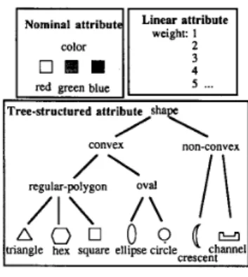
attribute-based instance space, each instance can be represented by one or several attributes. Each attribute may be nominal, linear, or tree-structured [30] (Fig. 1). For example, instance “color = red, weight = 1, shape = oval” is attribute- based. Attribute-based instance spaces are of the main concem here.

A hypothesis space is a set of hypotheses that can be legally described by a concept description language (generalization language). The most prevalent form of a hypothesis space is restriction to concepts that can be expressed only in conjunc-

1041-4347/94$04.00 0 1994 IEEE

(2)

858 IEEE TRANSACTIONS ON KNOWLEDGE AND DATA ENGINEERING, VOL. 6 , NO. 6 , DECEMBER 1994

Tree-structured attribute sha

/ \

non-convex I

I convex

Fig. 1. Attribute domain.

tive forms. For example, hypothesis “color = red and shape = convex” are in conjunctive forms. Because some unsolved problems in learning disjunctive concepts based on version space strategy [4], [20] still exist, the hypothesis spaces here are restricted to conjunctive forms.

Given an instance space and a hypothesis space, a set of predicates is still required to test whether a given hypothesis matches a given instance (i.e., whether the given instance is contained in the instance set corresponding to the given hypothesis). For example, in a tree-structured attribute domain, one matching predicate is a predecessor-successor relation in the hierarchy tree. In other words, a hypothesis matches an instance if the instance is a successor of the hypothesis in the hierarchy tree.

Two partial ordering relations, called ‘:more-specijic-than”

(I)

and “more-general-than”

B and A’ 5 C ,

then ’ ( A

5

A ’ ) .

The learning problem to be solved in this paper can now be defined as in [20].

Given the following information: 1) instance space,

2) hypothesis space,

3) a set of predicates to test whether a given hypothesis

4) a set of positive and negative training instances of a

determine one or several hypotheses in conjunctive forms, each of which is consistent with the presented training instances.

The term “consistent” means that this hypothesis matches

(includes) all given positive training instances and matches no (excludes) given negative ones.

matches a given instance, and

target concept to be learned,

Example 1: Consider the learning problem of classifying

examples belonging to different kinds of iris flowers [6], [lo]. Assume that the following information is given.

Instance Space: Each training instance is described by

four attributes-Sepal Width (S.W), Sepal Length (S.L), Petal Width (P.W), and Petal Length (P.L). Units for all the four attributes are centermeter, measured to the nearest millimeter.

Hypothesis Space: Each legal hypothesis is restricted to

be conjunctions of form a 5 X

<

b (for each attribute X ) , where a and b are limited to multiples of 8 mm.

Matching Predicates: A hypothesis H matches a training

0.8) is desired. Methods in achieving the

boundaries are discussed in the next section.

111. OVERVIEW OF VERSION SPACE LEARNING STRATEGY Version space leaming strategy [ 191, [20] was proposed by Mitchell in 1978, having been applied successfully in some systems such as Meta-DENDRAL [3] and LEX [23]. The term “version space” is used to represent all legal hypotheses

describable within a given concept description language and consistent with all observed training instances. A version space can be represented by two sets of hypotheses: set S and dual

set G, defined as follows.

S = {s

I

s is a hypothesis consistent with observed instances. No other hypothesis exists that is both more specific than s and consistent with observed instances};

G = {g

I

g is a hypothesis consistent with observed instances. No other hypothesis exists that is both more general than g and consistent with observed instances}.

Sets S and G together precisely delimit the version space, and each hypothesis in the version space is both more general than some hypothesis in S and more specific than some

hypothesis in G. When a new positive training instance appears, set S is generalized to include this training instance;

when a new negative training instance appears, set G is specialized to exclude this training instance. An example is given below to clearly explain version space strategy.

Example 2: For the learning problem given in Example 1, learning process by version space strategy is shown in Fig. 2.

In the newly formed version space by Step 3 (Fig. 2), (7.2

5

S.L

<

OO,o.o

5 s.w

(3)

HONG AND TSENG: LEARNING CONCEPTS IN PARALLEL 859

1. (S.L=5.1, S.W=3.5, P.L=1.4, P.W=0.2) Positive traznzng instance

S: (4.8<S.L<5.6, 3.2<S.W<4.0, 0.8<P.L<1.6, O.O<P.W<O.8) G: (O.O<S.L<m, O.O<S.W<m, O.O<P.L<m, O.O<P.W<m)

2. (S.L=4.3, S.W=3.0, P.L=1.1, P.W=O.l) Posatzve traznzng znstance S: (4.0(S.L<5.6, 2.4<S.W<4.0, 0.8(P.L<1.6, O.O(P.W<0.8) G: (O.O<S.L<m, O.O<S.W<m, O.O<P.L<m, O.O<P.W<m)

3. (S.L=7.0, S.W=3.3, P.L=4.7, P.W=1.4) Negatzve traznzng instance S: (4.0(S.L<5.6, 3.2<S.W<4 0, 0.8<P.L<1.6, O.O<P.W<0.8) G: (O.O<S.L<6.4, O.O<S.W<m, O.O<P.L<m, O.O<P.W<m)

(7.21S.L<m, O.O<S.W<m, O.O<P.L<m, O.O<P.W<m) (O.O<S.L<m, O.OSS.W<3.2, O.O<P L<m, O.O<P.W<m) (O.O<S.L<m, 4.0<S.W<m, O.O<P.L<m, O.O<P.W<m) (O.O<S.L<m, O.O<S.W<m, O.O<P L<4.0, O.O<P.W<m) (O.O<S.L<m, O.O<S.W<m, 4.8<P.L<m, O.O<P.W<m) (O.O<S.L<m, O.O<S.W<m, O.O_(P.L<m, O.O<P.W<O.8) (O.O<S.L<m, O.O<S.W<m, O.O<P.L<m, l.G<P.W<m) Fig. 2. Illustration for the version space strategy.

S/G must be more specific/general than at least one hypothesis in G/S.

Proofi Assume some hypothesis s in S is not more

specific than any hypothesis in G. According to the definition of version space, each hypothesis in the version space V must be more specific than some hypothesis in G and more general than some hypothesis in S. s is then not in V, implying that

s is not in S . A contradiction arises. Each hypothesis in S

must then be more specific than at least one hypothesis in G. U In parallel processing, coping with the synchronization problem is difficult if dependency among different processors is heavy [I], [26]. Because of the characteristic of not checking past training instances, the strategy of version space is suitable for rocessing in parallel.

Similar arguments can be given for G.

I v . LEARNING CONCEPTS IN PARALLEL

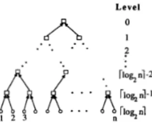
By applying similar idea used in DADO [9], 1291, a parallel learning model adopted is shown in Fig. 3. Each circle represents a training instance, and each rectangle represents a processing element.

All processing elements on the same level of the tree can work concurrently and in parallel. Learning process starts from the bottom rectangular level of the tree. At the beginning, each processing element inputs two separate training instances, finds sets S and G, which are defined in version space strategy,

and forms a version space as output. Each processing element lying on one level higher than the previous one then inputs two version spaces, processing them in order to form an equivalent version space as output. This process is repeated along with the tree bottom-up until a final version space is obtained.

Level 0

. .

A

. .

I

. .

_z

. .

Fig. 3, Bottom-up processing in a binaly tree.

A . Merging Two Version Spaces

The following lemma shows version space strategy allowing a convenient, consistent method for merging several sets of hypotheses generated from distinct training data sets [20].

Lemma 2: Intersection of two version spaces formed from two sets of training instances yields the version space consistent with the union of these two training sets.

Proof: Let Vl and V2 denote two original version spaces;

I1and I2 denote corresponding training sets. Since each hypothesis in VI matches all positive training instances and no negative training instances in 11, and because each one in V2 matches all positive training instances and no negative training instances in 1 2 , a hypothesis lying in both VI and

V2 must match all positive training instances and no negative training instances in I1 and Iz. Intersection of VI and V2 must

0

Corollary 1: Let intersection of two version spaces, formed

from two given training sets I1 and 1 2 with I = I1U 1 2 , be V. Intersection of two other version spaces, formed from two training sets 1, and

I4

with I = 13 U 14, is then still V.

The following two lemmas can be used to find intersection of two version spaces.

Lemma3: For each hypothesis s/g in S / G of the newly formed version space V from VI and V2, there must exist some hypothesis sl/gl in S 1 / G 2 and 5 2 / 9 2 in S 2 / G 2 such that s/g is a lgg/lss of s l / g l and s 2 / g 2 .

Proofi Without loss of generality, we need to prove only

the case for a hypothesis s in S . According to definition of S ,

no other hypothesis exists more specific than s in V. Since V is the intersection of VI and V2, s must be more general than some hypothesis s1 in

SI

and some s 2 in 5’2. Furthermore,

s must be a lgg of both s1 and sa; otherwise, there exists a hypothesis in V that is more specific than s , contradicting the

fact s is in S .

0

Inverse statement of Lemma 3 is.not always true. A lgg/lss

of some sl/gl in S1/G1 and some 5 2 / 9 2 in S 2 / G 2 is not necessarily in S/G. It may be subsumed by some other

hypotheses in the same set or may contradict hypotheses in the dual set.

Lemma 4 : For hypothesis s/g that is a Igg/lss of some hypothesis sl/gl iryS1/G1 and s ~ / g 2 in S 2 / G 2 , and another hypothesis s’/g’ that is a lgg/lss of another hypothesis si/g: in S1/G1 and sh/g& in S 2 / G 2 , if s / g is more specific/general than s’lg’, then s‘/g‘ will not be in S/G.

Proof: Without loss of generality, only the case for S needs to be proven. If s is in S, s’ will not then be in S ,

(4)

860 IEEE TRANSACTIONS ON KNOWLEDGE A N D DATA ENGINEERING, VOL. b, NO. b. DECEMBER 1994

according to the definition of S. I f s is not in S, it cannot then find any hypothesis in G more general than it, according to Lemma 1. Since s is more specific than s’, s’ cannot find any hypothesis in G more general than it neither. s’ cannot be in According to Lemma 3, the set (named S’ ) that contains desired set S can be found by taking each hypothesis in S1 and each in SZ to generate the lgg’s of the pair of chosen hypotheses. A Generalization process is defined here as the process of

finding the lgg ’s of two chosen hypotheses. A Specialization process is similarly defined as the process of finding the lss’s

of two chosen hypotheses. Besides, Lemma 4 introduces an additional processing, redundancy and subsumption checking,

in excluding the redundant and not least general hypotheses in S’. The process is similar for set G. After redundancy and subsumption checking, another type of checking called

contradiction checking needs to be performed in discarding the hypotheses in S I G that is not more specific/general than any hypothesis in G / S due to Lemma 1.

Generally assume that two version spaces VI and V2 exist, where corresponding

S2 are obtained. Redundancy, subsumption, and contradiction

checking, meanwhile, should be done among newly formed hypotheses in S and G. Merging of G sets can be processed in a similar way.

B . Parallel Learning Algorithm

Parallel algorithm for concept learning can be outlined below from the above discussion. This is basically based upon the principle of divide-and-conquer [ 161, [27].

Parallel Learning Algorithm:

INPUT: A set I of n training instances.

OUTPUT: A version space V with sets S and G consistent with the set

I.

STEP 1: Divide I into I1 and 12. The sizes of I1 and I2 are equal. (If the size of I is not even, add a virtual training instance to I to make the size even.) Besides, the distributions of positive and negative training instances in

11 and 12 are as equal as possible.

STEP 2: Recursively and in parallel apply the algorithm to find the version space VI for 11 and V, for 1 2 , respectively.

STEP 3: Merge the two version spaces VI and V2 into an equivalent version space V.

The version space for a virtual training instance here is the universal version space with S equal to the most specific hypothesis and G equal to the most general hypothesis in the hypothesis space. From Corollary 1, any partition of I will not affect correctness of the final version space. It indeed affects

intermediate results, however, and then influences learning speed. By interleaving positive and negative training instances as much as possible, illegal hypotheses in S and G can be removed as early as possible. The needed learning time is then shorter. This is illustrated by the experiments in Section VII. Each positive training instance can initially be viewed as a version space with set S containing only the instance itself; each negative training instance can be viewed as a version space with set G excluding only the instance itself. The merging algorithm is then described as follows:

Version Space Merging Algorithm:

INPUT: Two version spaces VI with

SI,

G I , and V, with

Sa, Ga.

OUTPUT: An equivalent version space V with S and G. STEP 1: Initialize both sets S and G to be

4.

STEP 2: Take a hypothesis in SI and a hypothesis in Sz (in an order of (1, l), (1, 2), .e., (1, ( S Z ~ ) , (2, I), (2, 2), .-.,

(2, ( S Z ~ ) , .

.

.,

ClSll,

l), (IS,(, 2), . . .(IS,(,

(SZ(),

where

1x1

denotes cardinality of set X) to perform a generalization process. Set newly formed hypotheses to be SI. Check S’ with S against redundancy and subsumption with three cases possibly existing.

Case 1. If a hypothesis s’ in S’ is more general than some hypothesis s in S, discard s‘ in S’. Case 2. If a hypothesis s’ in S’ is more specific

than some hypothesis s in S, discard s and add

s’ to set S.

Case 3. Otherwise, add s’ to set S .

STEP 3: Repeat STEP 2 until each hypothesis in

SI

is processed with each hypothesis in Sa.

STEP 4: Take a hypothesis in GI and a hypothesis in G2 (in an order of (1, I), (1,2),

.

.,

(1, ( G z ~ ) , (2, I), (2,2), .

. .,

(2, IGzI), .

.

., <lG1(, l), (lG11, 2), . . -(lG,l, IG2))) to perform a specialization process. Set newly formed hypotheses to be GI. Check G‘ with G against redundancy and subsumption with three cases possibly existing.

Case 1. If a hypothesis g’ in G’ is more specific than some hypothesis g in G, discard g’ in G‘. Case 2. If a hypothesis g’ in G’ is more general than some hypothesis g in G, discard g and add

g‘ to set G.

Case 3. Otherwise, add g’ to set G.

STEP 5: Repeat STEP 4 until each hypothesis in G1 is processed with each hypothesis in G2.

STEP 6: Take a hypothesis s in S and a hypothesis g in G (in an order of (1, l), (1, 2),

...,

(1, /GI), (2, l), (2, 2), .e.,

(2, )GI),

. . .,

(ISl, I),

((SI,

2),

.

-(JSl, JGI)). Check s with g against contradiction with two cases possibly existing.

Case 1. If g is not more general than s, mark s and g.

(5)

HONG AND TSENG: LEARNING CONCEF'TS IN PARALLEL 86 I

STEP 7: Repeat STEP 6 until each hypothesis in S is processed with each hypothesis in G.

STEP 8: Discard those hypotheses in S with (GI marks and

those in G with IS( marks.

After execution of Step 8, the desired version space is obtained. Note in Case 1 of Step 2/Step 4, the process includes checking of redundancy. This is because more-specific-than and more-general-than relations have the reflexive property. Correctness of our algorithm is shown below.

Theorem 1: The version space obtained by the version

space merging algorithm here is the intersection of two given original version spaces.

Proof: Let S" denote set S obtained after Step 3, and let G" denote set G obtained after Step 5 for the sake of

clarity. Because of Step 2, in generated hypotheses, only the least general ones are kept, such that each hypothesis in S"

is not more general than the others. According to Lemmas 3 and 4, S" is a superset of the final S. S" can then be divided

into two disjoint sets: the final S and SI'-S. It implies that any hypothesis in SI'-S is not in the final version space and is not more specific than ,any hypothesis in G by Lemma 1.

Otherwise, some hypothesis in SI'-S must be in S. Set GI'

after STEP 5 can similarly be divided into the final set G

and G"-G. In Step 6 to Step 8, S" and G" are checked for

contradiction and G"-G and 5'"-S will be discarded after Step 8. After Step 8, the final sets G and S are then desirable. 0

It can easily be seen that Steps 2 and 3 can be performed in parallel; Steps 4 and 5 and Steps 6 to 8 are also the same cases. The merging algorithm described above can then be further parallelized if q free processors are available.

Parallel Version Space Merging Algorithm:

INPUT: Two version spaces VI with

SI,

G I , and V2 with S2, G2.

OUTPUT: An equivalent version space V with S and G.

PSTEP 1: In each processor P;, initialize both sets SPi and PSTEP 2: Divide and assign

(SI

I

hypotheses of

SI

(without loss of generality, assume

(SI

I

2 I&()

as equally as possible onto the available q processors. Refer to the set in

P;

as

SP1;. In each processor Pi, take a hypothesis in SPli and

a hypothesis in S2 to perform a generalization process.

Set newly formed hypotheses to be SP,!. Check SP,! with

SP; against redundancy and subsumption with three cases

GPi to be

4.

possibly existing.

Case 1. If a hypothesis s' in SP: is more general

than some hypothesis s in SP;, discard S I in SP,!.

Case 2. If a hypothesis s' in SP,! is more specific

than some hypothesis s in SPi, discard s and add s' to set SPi.

Case 3. Otherwise, add S I to set SP;.

Repeat this step until each hypothesis in SPI; is processed

with each hypothesis in S2.

PSTEP 3: Pairwise and in parallel, merge-check SP1, SP2,

. . .,

SP, against interprocessor redundancy and subsumption by the bottom-up way (Fig. 4). In each intermediate

processor for managing sets SP; and SPj, check each

hypothesis S I in SP; with SPj, with three cases possibly

existing.

Case 1. If S I is more general than some hypothesis

s in SPj, discard s' in SPi.

Case 2. If S I is more specific than some hypothesis

s in SPj, discard s and add s' to set SPj.

Case 3. Otherwise, add s' to set SPj.

Output SPj upward for further merge-check. Refer to the set output at Level 0 as SI.

PSTEP 4: Divide and assign IG1

I

hypotheses of G1 (without

loss of generality, assume 1G11 2 1G21) as equally as

possible onto the q available processors. Refer to the set in Pi as GP1;. In each processor Pi, take a hypothesis in GPl; and a hypothesis in G2 to perform a specialization

process. Set newly formed hypotheses to be GP,!. Check GP,! with GP; against redundancy and subsumption, with

three cases possibly existing.

Case 1. If a hypothesis g1 in GP,! is more specific

than some hypothesis g in GP;, discard g' in GP,!.

Case 2. If a hypothesis g1 in GP,! is more general

than some hypothesis g in GPi, discard g and add

g' to set GP;.

Case 3. Otherwise, add g1 to set GPi;

Repeat this step until each hypothesis in GP1; is processed

with each hypothesis in G2.

PSTEP 5: Pairwise and in parallel, merge-check GP1, GP2,

. .

., GP, against interprocessor redundancy and subsump-

tion by the bottom-up way (Fig. 4). In each intermediate processor for managing sets GP; and GPj, check each

hypothesis g' in GPi with GPj with three cases possibly

existing.

Case 1. If g' is more specific than some hypothesis g in GPj, discard g' in GP;;

Case 2. If g' is more general than some hypothesis g in GPj, discard g and add g' to set GPj.

Case 3. Otherwise, add g' to set GPj.

Output GPj upward for further merge-check. Refer to the

set output at Level 0 as GI.

PSTEP 6: Divide and assign JG'J hypotheses of GI (without

loss of generality, assume /GI( 2

IS'/)

as equally as possible onto the available q processors. Refer to the set in P; as

G:. In each processor Pi, check each hypothesis s in S'

with each hypothesis g in G: against contradiction with two

cases possibly existing.

Case 1. If g is not more general than s, mark s and g.

Case 2. Otherwise, do nothing.

Repeat this step until each hypothesis in S' is processed with each hypothesis in G:. Discard those hypotheses in G!,

(6)

862 IEEE TRANSACTIONS ON KNOWLEDGE AND DATA ENGINEERING, VOL. 6, NO. 6 , DECEMBER 1994 Level 0

. .

A

. .

I ?

. .

. -

Fig. 4. Illustration for parallel merging.

PSTEP 7: Pairwise and in parallel, count the total number of marks of each hypothesis s in S’ by the bottom-up way (Fig. 4). Discard the hypotheses of S’ with IG’l marks,

referring to the altered set as S .

Theorem 2: The version space obtained by the parallel version space merging algorithm here is the intersection of two given original version spaces.

Pro08 It can easily be proven that each intermediate

result at end of PSTEP 3, PSTEP 5, and PSTEP 7 of the parallel merging algorithm is, respectively, the same as that at end of STEP 3, STEP 5, and STEP 8 of the sequential merging algorithm. After PSTEP 7, sets S and G then constitute the

Theorem 3: The parallel version space learning algorithm

is correct.

Proof: According to Theorems 1 and 2, correctness of our parallel learning algorithm can easily be proven by

desired version space.

0

G: (0- $3- 00 ,0-- ,0-0.8) ,0-00 .0- 4.0.0- m ) (0- (0-6.4 ,0- m ,0- 0- 0 0 ) ( 1 ) S: (4.0-5.6, 2.4-4.0.0.8-1.6.0-0.8)

/

\

G: (O-=,O-m,O-m ,0-0.8) (0-00 ,O-m ,0- 4.0.0-- ) (0-6.4 ,0-

-

,0--, 0- 0 0 ) G: (0-- ,0-m,0-- ,0-1.6) (0-00 ,0-m ,0- 4.8.0-m ) (0-6.4 ,0- ,&=, 0- m ) S: (4.8-5.6, 3.2-4.0, 0.8-1.6, 0-0.8) S: (4.0-4.8. 2.4-3.2.0.8-1.6, 0-0.8)

f

2

(5.1,3.5,1.4,0.2,+) (7.0,3.3,4.7,1.4,-) (4.3,3.0,1.1,0.1,+) (6.4,2.7,5.3,1.9,-) G: (0-- ,0- m .0- ,0-0.8) (Gm ,0-00,0-3.2,0-m) ( 2 ) (0- ,3.2-m ,0-m, 0- m ) S: (4.8-6.4, 3.2-4.8.0.8-2.4, 0-0.8)

/

\

G: ,O-m,O-m ,0-0.8) ( G m ,&m ,0-m ,&1.6) (0- m .&a, ,0- 4.8.0- m ) (0-00 ,0- .0- 3.2.0- m ) (O-m,3.2--,0--.0--) ( 0 - - , 3 . 2 - m , 0 - m , 0 - m ) (5.6- S: (5.6-6.4, 4.0-4.8, 0.8-1.6,0-0.8) S: (4.8-5.6, 3.2-4.0, 1.6-2.4.0-0.8) ,0-

-

,0- 00.0- m )

/ 2*

f

Z

(5.7,4.4,1.5,0.4,+) (5.2.2.7.3.9J.4,-) (4.8,3.4,1.9,0.2,+) (5.5,2.8,4.9,2.0,-) G: (0-00 ,0-- ,O-m ,0-0.8) (0-- ,0-m ,0- 3.2.0-00 ) S: (4.0-6.4, 2.4-4.8.0.8-2.4, 0-0.8)

f

Z

( 1 ) ( 2 )

Fig. 5. Illustration of parallel version space strategy.

induction.

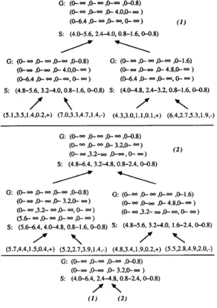
Example 3: For the learning problem described in Example 1, assume the training set is given as follows:

positive instances: (5.1, 3.5, 1.4, 0.2), (4.3, 3.0, 1.1, O.l), (5.7, 4.4, 1.5, 0.4), and (4.8, 3.4, 1.9, 0.2),

negative instances: (7.0, 3.3,4.7, 1.4), (6.4, 2.7, 5.3, 1.9), (5.0, 2.7, 3.9, 1.4), and (5.5, 2.8, 4.9, 2.0).

Parallel learning process by version space strategy is shown in Fig. 5; each notation a N b represents a

5

X

<

b for value

X of some attribute.

V. TIME COMPLEXITY ANALYSIS

Checking is used for examination of redundancy, subsumption, and contradiction among hypotheses in sets S and G. Checking

between any two hypotheses can be finished within a unit operation, because it is simpler than a specialization process or a generalization process.

We now focus on time complexity analysis of our parallel learning algorithm. Let T p ( n ) denote time complexity of our parallel learning algorithm in dealing with n training instances

with q processors available (assume n

5

q; the case for n

>

q

is discussed in Section VI). Let M,(n) denote time complexity of merging two version spaces VI and V2, each of which is In this section, time complexities of our parallel learning

Mitchell [20], [22] are analyzed and compared. For the purpose

formed from n/2 training instances, into an equivalent version environment, the following formula holds:

algorithm and the sequential learning algorithm proposed by space with q processors In this parallel leaming of having a criterion about processing time, a unit operation

is defined below.

Definition:

Unit operation: A specialization or generalization process from any two chosen hypotheses is defined as a unit operation.

ne

unit operation defined above, most likely as the time unit in Mitchell’s sequential learning analysis [20], is from here on considered as a basic time unit of

In analyzing time complexity of M q ( n ) , let smax and g m a x , respectively, denote the maximum numbers of hypotheses in Sets

s

and G appearing in the whole leami% process. For the parallel merging algorithm outlined in Section IV, the time complexity of each step is listed in Table I. Therefore, we have the

processing.

For the merging algorithm proposed in Section IV-B, processing time includes the required number of specializa-

~ q ( n ) = O ( s 3 , a x / q

+

’:ax [log2 41

+

d a x / q

+

g L a x [log2 41 )

+

s m a x x g m a x / q

(7)

863

HONG AND TSENG: LEARNING CONCEPTS IN PARALLEL

TABLE I

In this case, time complexity is arrived at by

calculating as’ follows:

Time complexity of the sequential algorithm proposed by Mitchell [20], [22] is given as follows:

~ 1 ( n ) = O(smax x gmax x n

+

s2,ax x P

+

giax x

F ) ,

( 5 )

where p represents the number of positive instances,

p

represents the number of negative instances, and p

+

j3 = n. Some related remarks about the time complexity analysis are discussed below.

Numbers df training instances

Fig. 6. Typical relation of version space boundary set sizes to numbers of

training instances.

6) The maximum numbers Smax and gmax of hypotheses in sets S and G can generally be characterized by the following entities:

smax = Function, ( P , N , 0 ) ,

gmax = Function, ( P , N , O ) ,

where

P = the particular learning problem considered, N = the number of training instances, and

O= the order in which training instances are arranged.

Interleaving positive and negative training instances can make illegal hypotheses in S and G removed as early as possible in the contradiction checking. phase; it is then the best arrangement of training instances. By interleaving positive and negative training instances, the following equation can then be derived:

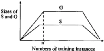
Mitchell also showed that the sizes of S and G typically behave as shown in Fig. 6 [20]. When n is large

( 2

n'), then we have the following:

s ,

, = Function: ( P ) , gmax = Function; ( P )

.

In the parallel learning algorithm for large n, smax and gmax

then depend only on the leaming problem.

Mitchell further pointed out for the feature interval learning problem as in Example 1, S can never contain more than one hypothesis, and the size of G is usually small [20]. Experiments in Section VI1 show this.

VI. A BOUNDED NUMBER OF PROCESSORS In the algorithm mentioned above, the leaming process needs n processors where n (the number of training instances)

may be very large. But in real applications, only a limited number of processors are available. It is then necessary to develop a parallel learning algorithm with only a bounded number of processors available.

Assume r ( < n ) processors are available, where r is a

constant. The modified parallel learning algorithm here for a bounded number of processors is divided into two phases. In Phase 1, n given training instances are equally divided and

placed on T processors, and the sequential leaming algorithm

runs on each processor to obtain its own version space. In Phase 2, the r version spaces are merged in a way of binary tree, as mentioned in Section IV. Time complexity of the modified algorithm can be easily analyzed as follows:

When the number of available processors increases, the time spent in Phase 1 will decrease; but the time spent in Phase 2 will increase. The time saved in Phase 1 will grow smaller and smaller along with the addition of processors, and, however, does not necessarily make up the additional overhead in Phase 2. It implies in getting to the maximum speedup, the number of processors is not necessarily to be n. The appropriate number r of processors (over which additional processors are useless

to increase speedup) can then be decided by the inequation

T T ( n )

5 TT/2(n),

and the following calculation is derived:

From (9), when n is larger, r is larger, too; speedup is then also larger.

VII. EXPERIMENTS

In demonstrating effectiveness of the proposed parallel version space learning algorithm, Fisher's Iris Data, containing 150 training instances, is used [6]. Since the data is inconsistent, two training instances are removed out of it to make it consistent, so that the final version space will not be empty. Managing noisy data by version space is beyond discussion here, and can be referenced in [lo], [12], [15].

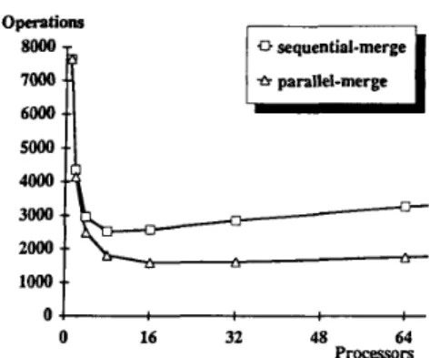
The Iris Problem has been introduced in Example 1. In fact, three species of Iris Flowers to be distinguished exist: setosa, versicolor, and verginica. Fifty training instances exist for each class. When the concept of setosa is learned, training instances belonging to setosa are considered as positive; training instances belonging to the other two classes are considered as negative. Similar management is applied in learning concepts of the other two classes. Execution of the parallel leaming algorithm is simulated at the IBM PC/AT (with communication time ignored). By running 100 times, execution time along with different numbers of processors (by the parallel merging algorithm) is shown in Fig. 7. For showing difference between using the parallel merging algorithm and using the sequential merging algorithm, versicolor's data is used as positive instances, with the result being as shown in Fig. 8. The numbers of operations calculated by (8) are also shown in Fig. 9. Sizes of smax and gmax are listed in Table 11.

From these figures, the following points can be observed. 1) From (9), when the number of processors is larger than a

(9)

HONG AND TSENG: LEARNING CONCEmS IN PARALLEL 865 Opentiom Seconds 160 140 TABLE I1 SIZES OF s , , , ~ , AND g,,,, Versicolor 8 + Set- a Viginica

*

Versicolor 60 40 20 0 16 32 48 64 PlWWORi Fig. 7. Execution time for Iris Learning Problem.

Seconds 140 120 100

I

0 Sequential-merge 0 Parallel-merge 40

L

2o 0

L

0 16 32 48 64 PlWWOrS Fig. 8. Execution time of different merging algorithms.

to reduce execution time. Substituting smax, gmax, n, p and

p

by 1, 8, 150, 50, and 100, respectively, in (9),

T is derived to be 16 (power of 2). The best speedup

then happens when 16 processors are used. Since (9) is analyzed by the worst case, the shape of curves in Fig. 7 can be thought to be quite consistent with theoretical analysis shown in Fig. 9.

2) From Fig. 8, difference of execution time in using the parallel merging algorithm and using the sequential merging algorithm increases when the number of available processors increases. When the number of processors increases, the merging steps increase and the saved time increases also.

3) The worst-case speedup by theoretical analysis based on (4) and (5) is about 3.92, being close to the empirical speedups, 4.33, 5.27, and 3.84 for these three classes.

"w

6000 5000

+I

*

parallel-merge - . 0 16 32 48 64 Processors

Fig. 9. Numbers of operations calculated by (8).

In comparison with the effect of interleaving positive and negative training instances, positive ones are arranged on one side, and negative ones are arranged on the other side. For this arrangement, gmax can get to 50 and execution time for the sequential learning algorithm can arrive to 69.22 s in average on Class setosa. Note that gmax is only 8 and execution time is only 1.678 s, on the average, for interleaving arrangement. Interleaving positive and negative training instances is then an effective way in reducing sizes of S and G and reducing execution time of the learning process.

At last, the original data is duplicated 10 times in forming a new set that contains 1500 training instances. The parallel learning algorithm and the sequential learning algorithm then run on the set and speedup is found to be 22.73. Theoretic speedup by (4) and (5) is 19.53. Comparing this result with that obtained from only 150 training instances, we can conclude that speedup will increase along with an increase of training instances.

VIII. CONCLUSION AND PROSPECTS FOR FUTURE WORK We have successfully applied the technique of parallel processing in the field of concept learning for raising the learning speed. We have proposed a parallel version space leaming algorithm based upon the principle of divide-and- conquer, and modified this parallel leaming algorithm, as a result of practical restrictions, to a bounded number of processors.

By theoretic analysis, we have found, with n processors, that

the learning process can be accomplished within O ( E ~ ----f c1

log,n

+

c ~ ) . Only T processors, which can be derived by

(9), are actually enough in achieving the maximum speedup. Our parallel learning algorithm has also been applied on the Iris Learning Problem in achieving a result quite consistent with our analysis. Effectiveness of interleaving positive and negative training instances is also verified.

One important point must finally be clarified here. Mitchell mentioned that when the current version space is incompletely learned, an informative new training instance that matches half the hypotheses in the current version space would be selected in the next leaming iteration [20]. A shortest number of training instances are then enough to make a version space

(10)

866 IEEE TRANSACTIONS ON KNOWLEDGE AND DATA ENGINEERING, VOL. 6. NO. 6, DECEMBER 1994

converge to a single hypothesis, thought of as the final concept. This strategy is good and effective for some learning problems; however, it is not totally suitable for the leaming problem defined in Section 11. In this paper, the learning problem to be solved is to find hypotheses consistent with given training instances. When the training instances are inconsistent or the description language is insufficient, the version space derived is null. A final version space with only a single hypothesis can always be derived by using only the shortest number of informative new training instances. This version space derived, however, cannot guarantee consistency with all the given training instances.

Besides, it may be not easy to find a training instance that matches half (or nearly half) the hypotheses in a version space. Mitchell proposed an effective heuristic for the feature interval leaming problems. In general, however, an analysis for a general learning problem is complex and costly [20]. Furthermore, even the training instance that matches half the hypotheses in the current version space can be derived, it may be out of the given training set. Methods for collecting additional training instances are then required, and the leaming job must then be delayed. As a better altemative than that, all the current training instances are processed. If a convergent version space or a null version space is derived, then the leaming process finishes; otherwise, the incompletely learned version space can also serve as a better classifier than that by the former altemative. Off-line knowledge acquisition is then performed, if possible, to find informative new training instances for further shrinking the incompletely learned version space.

We must then depend on the characteristics of the application domains to determine an appropriate learning strategy. If the given training instances are assured to be consistent, each informative new training instance is easily calculated from a version space, and if all possible instances exist in the given training set, then sequential learning by processing an informative new training instance at each iteration is good. Otherwise, processing all the given training instances would provide a better result, and parallel processing can then be well applied.

One disadvantage of the version space learning strategy is that it is sensitive to noise. When noise exists in the training set, the version space derived is usually null. Noise, however, exists in nearly all real-world application domains. Developing a new leaming strategy or modifying an existing leaming strategy for managing noise or uncertainty is then necessary. We have successfully proposed a generalized version space leaming strategy [12], [15] to handle training sets with noisy and uncertain instances. We are now trying to use the parallel leaming model for the kind of leaming problems.

For other models of parallel machine learning, we have applied the principle of task assignment to top-down leaming strategies [ 131. We have also applied the broadcasting communication model in simultaneously processing training instances in connectionist learning [14]. In the future, we will attempt to develop parallel models for other leaming methods and to implement them on various types of parallel architectures.

~-

ACKNOWLEDGMENT

The authors would like to thank C.-T. Yang for his assis- tance in performing these experiments. We would also like to thank the anonymous referees for their very constructive comments.

REFERENCES

[ I ] S. G. Akl, The Design and Analysis of Parallel Algorithms. Englewood

Cliffs, NJ: Prentice-Hall, 1989, pp. 1CL17.

[2] B. Arbab and D. Michie, “Generating rules from examples,” in Proc. 1985 Int. Joint Conf. Art. Intell., 1985, pp. 631-633.

[3] B.G. Buchanan and T.M. Mitchell, “Model-directed learning of production rules,” in D.A. Waterman and F. Hayes-Roth, Eds., Pattern- Directed Inference Systems. New York: Academic, 1978, pp. 297-3 12.

[4] A. Bundy, B. Silver, and D. Plummer, “An analytical comparison of some rule-learning programs,” Art. Intell., vol. 27, pp.,137-181, 1985.

[5] T. G. Dietterich and R. S. Michalski, “A comparative ‘review of se- lected methods for learning from examples,” in R. S. Michalski, J. G.

Carbonell, and T. M. Mitchell, Eds., Machine Learning: An Artificial Intelligence Approach, vol. 1. Palo Alto, CA: Toiga, 1983, pp. 41-81.

[6] R.A. Fisher, “The use of multiple measurements in taxonomic problems,” Ann. Eugenics, vol. 7, pp. 179-188, 1936.

[7] L.M. Fu and B.G. Buchanan, “Learning intermediate concepts in constructing a hierarchical knowledge base,” in Proc. 1985 Int. Joint

Conf Art. Intell., 1985, pp. 6 5 9 4 6 6 .

[8] S. I. Gallant, “Automatic generation of expert systems from examples,” in Proc. 2nd Int. Conf. Art. Intell. Applications, 1985, pp. 313-319.

[9] A. Gupta, “Implementing OPS5 production systems on DADO,” in Proc.

1984 IEEE Int. Con$ Parallel Processing, 1984, pp. 83-91.

[ 101 H. Hirsh, “Incremental version-space merging: a general framework for concept learning,” Ph.D. dissertation, Stanford Univ., Stanford, CA, USA, 1989.

[ 1 I] T. P. Hong and S. S. Tseng, “A parallel concept learning algorithm based upon version space strategy,” in Proc. 1990 IEEE Int. Phoenix Cor$ Comput. Commun., 1990, pp. 734-740.

[I21 -, “A generalized learning problem,” in Proc. 1990 Inc. Comput. Symp., 1990, pp. 517-522.

[I31 -, “Models of parallel learning systems,’’ in Proc. 1991 IEEE Int.

Conf. Distrib. Computing Syst., 1991, pp. 125-132.

[ 141 -, “Parallel perceptron learning on a single-channel broadcast communication model,” Parallel Computing, vol. 18, pp. 133-148,

1992.

[15] T.P. Hong, “A study of parallel processing and noise management on machine learning,” Ph.D. dissertation, National Chiao Tung Univ., Taiwan, Republic of China, Jan. 1992.

(161 E. Horowitz and S. Sahni, Fundamentals of Computer Algorithms.

New York: Computer Science Press, 1978, pp. 98-140.

[17] R. S. Michalski, J. G. Carbonell, and T. M. Mitchell, Machine Learning: An Artificial Intelligence Approach, vol. 1. Palo Alto, CA: Toiga, 1983. [ 181 -, Machine Learning: An Artificial Intelligence Approach, vol. 2.

Palo Alto, CA: Toiga, 1984.

[ 191 T. M. Mitchell, “Version space: a candidate elimination approach to rule learning,’’ in Proc. 1977 Int. Joint Con$ Art. Intell., 1977, pp. 305-310.

[20] -, “Version spaces: An approach to concept learning,’’ Ph.D. dissertation, Stanford Univ., Stanford, CA, USA, 1978.

[21] -, “An analysis of generalization as a search problem,” in Proc. 1979 Int. Joint Conf. Art. Intell., 1979, pp. 577-582.

[22] -, “Generalization as search,” Art. Intell., vol. 18, pp. 203-226,

1982.

[23] T.M. Mitchell, P.E. Utgoff, and R. Banerji, “Learning by experi- mentation: Acquiring and refining problem-solving heuristics,” in R. S. Michalski, J. G. Carbonell, and T. M. Mitchell, Eds., Machine Learning: An Artificial Intelligence Approach, vol. 1. Palo Alto, CA: Toiga, 1983,

[24] G. D. Plotkin, “A note on inductive generalization,” in B. Meltzer and D. New York: Wiley, 1970, [25] -, “A further note on inductive generalization,” in B. Meltzer and New York: Wiley, 1971, [26] M. J. Quinn, Designing Ejjicient Algorithms f o r Parallel Computers.

[27] R. C. T. Lee, R. C. Chang, and S. S. Tseng, Introduction to Design and

pp. 163-190.

Michie, Eds., Machine Intelligence, vol. 5.

pp. 153-163.

D. Michie, Eds., Machinelntelligence, vol. 6.

pp. 101-124.

New York: McGraw-Hill, 1987.

(11)

HONG AND TSENG: LEARNING CONCEPTS IN PARALLEL 867

[28] M. J. Shaw, “Applying inductive learning to enhance knowledge-based expert systems,” Decision Support Syst., vol. 3 , pp. 319-332, 1987. [29] S. J. Stolfo and D. P. Miranker, “DADO: A parallel processor for expert

systems,” in Proc. I984 IEEE Int. Con5 Parallel Processing, 1984, pp.

74-82.

[30] L. H. Witten and B. A. Macdonald, “Using concept learning for knowledge acquisition,” Int. J. Man-Mach. Studies, vol. 29, pp. 171-196, 1988.

Hua Polytechnic Institute interests include parallel 1 set, and expert systems.

T.-P. Hong received the B.S. degree in chemical engineering from National Taiwan University in 1985, and the Ph.D. degree in computer science and information engineering from National Chiao Tung University in 1992.

Since 1987, he has been with the Laboratory of Knowledge Engineering, National Chiao Tung University, where he has been involved in applying techniques of parallel processing to artificial intelligence. He is currently an Associate Professor at the Department of Computer Science at Chung-

’ in Taiwan, Republic of China. His current research

processing, machine learning, neural networks, fuzzy

S . 4 . Tseng (M’88) received the B.S., M.S., and Ph.D. degrees in computer engineering from Na- tional Chiao Tung University in 1979, 1981, and 1984, respectively.

Since August 1983, he has been on the faculty of the Department of Computer and Information Science, National Chiao Tung University, and is currently a Professor there. From 1988 to 1991, he was the Director of the Computer Center at National Chiao Tung University, Taiwan, Republic of China.

From 1991 to 1992, he acted as the Chairman of the Department of Computer and Information Science. Now he is the Director of the Computer Center at the Ministry of Education, Republic of China. His current research interests include parallel compiler, language processor design, computer algorithms, parallel processing, and expert systems.

Dr. Tseng is an Associate Editor of Informarion and Education, and a member of the International Advisory Board of CISNA COMPUTER FORUM. He was elected an Outstanding Talent of Information Science of the Republic of China in 1989. He was also awarded the Outstanding Youth Honor of the Republic of China in 1992.