Exact number of mosaic patterns in cellular neural networks

(1)

c

World Scientific Publishing Company

EXACT NUMBER OF MOSAIC PATTERNS IN

CELLULAR NEURAL NETWORKS

JUNG-CHAO BAN, SONG-SUN LIN∗ and CHIH-WEN SHIH∗,†

Department of Applied Mathematics, National Chiao Tung University, Hsinchu, Taiwan, R.O.C.

Received February 10, 2000; Revised December 15, 2000

This work investigates mosaic patterns for the one-dimensional cellular neural networks with various boundary conditions. These patterns can be formed by combining the basic patterns. The parameter space is partitioned so that the existence of basic patterns can be determined for each parameter region. The mosaic patterns can then be completely characterized through formulating suitable transition matrices and boundary-pattern matrices. These matrices gener-ate the patterns for the interior cells from the basic patterns and indicgener-ate the feasible patterns for the boundary cells. As an illustration, we elaborate on the cellular neural networks with a general1× 3template. The exact number of mosaic patterns will be computed for the system with the Dirichlet, Neumann and periodic boundary conditions respectively. The idea in this study can be extended to other one-dimensional lattice systems with finite-range interaction.

1. Introduction

The cellular neural network (CNN) proposed by Chua and Yang [1988a, 1988b] is a large aggrega-tion of analogue circuits. The system presents

it-self as an array of identical cells Ci which are

lo-cally coupled. In this study, we consider the CNN with cells coupled in a one-dimensional fashion (1-d CNN). Assume that the cells are sitting on the

lattice Tn := {i ∈ Z1|1 ≤ i ≤ n}. The governing

equation for the cell Ci at the site i, i ∈ Tn, takes

the form dxi dt =−xi+ X 1≤|k|≤r βkf (xi+k) + af(xi) + z , (1)

where xi+k, i + k /∈ Tn, satisfies certain boundary

condition to be described below. Herein, the output function f is a piecewisely linear function given by

f (ξ) = 1

2(|ξ + 1| − |ξ − 1|) ,

and yi = f (xi) is the output for the cell at i. In

addition, z is a time-independent bias and r is a positive integer indicating the radius of connection

between cells. The coupling parameters βk and a

constitute a space-invariant 1× (2r + 1) template

Ar. Namely,

Ar = [β_−r· · · β−1 a β1· · · βr] .

We denote by Nr(i) = {k|i − r ≤ k ≤ i + r} the

neighbors of the cell Ci, which are within the range

of connection for Ci. A practical CNN has finitely

many cells. Hence, the boundary condition (B.C.) has to be imposed and realized. We shall consider three types of boundary conditions in this presenta-tion; namely, the Dirichlet, Neumann and periodic

boundary conditions. These conditions are

illus-trated for 1-d CNN with r = 1 as follows. Dirichlet B.C.:

The absent cell x0(resp. xn+1) on the left-hand side

∗_{The authors are supported, in part, by the National Science Council of Taiwan, R.O.C.} †_{Author for correspondence.}

E-mail: [email protected]

1645

Int. J. Bifurcation Chaos 2001.11:1645-1653. Downloaded from www.worldscientific.com

(2)

of x1 (resp. the right-hand side of xn) are set to constants. Namely,

x0(t) = ˜x0, xn+1(t) = ˜xn+1.

The situation that the imposed boundary data ˜x0

and ˜xn+1 have their absolute values greater than

one is represented by D1-B.C., while the case ˜x0=

˜

xn+1= 0 is denoted by D0-B.C.

Neumann B.C.:

It is the zero-flux or reflective B.C., i.e.

x0(t) = x1(t) , xn+1(t) = xn(t) .

Periodic B.C.:

Two ends of Tn are connected to form a circular

array. Namely,

x0(t) = xn(t) , xn+1(t) = x1(t) .

Let x = (x1, x2, . . . , xn) be a stationary

so-lution of (1). The associated output y = (y1,

y2, . . . , yn) with yi = f (xi) is called a (stationary)

pattern. The stationary solutions and patterns can be classified into four types: mosaic, defect, inte-rior, and transitional, as defined in [Juang & Lin, 2000]. Herein, the definitions of the mosaic solu-tions and patterns which are the main concerns in this work are recalled. They are slightly modified to fit in the context of this study, that is, on the solutions and patterns on “finite” lattice.

Definition 1.1. A stationary solution x = (x1,

x2, . . . , xn) of (1) is called a mosaic solution if

|xi| > 1 for all i ∈ Tn. Its associated (output)

pattern is called a mosaic pattern.

Notably, the mosaic solutions of CNN were called stable system equilibrium points in [Chua & Yang, 1988]. These mosaic solutions are all stable

on finite lattice and on infinite lattice.

Further-more, under certain conditions on the parameters, every solution tends to a mosaic solution as time tends to positive infinity, cf. [Lin & Shih, 1999]. Our approach of constructing mosaic patterns on

Tn for (1) is to combine the basic patterns and

form patterns on larger lattices, as discussed in [Shih, 1998] and [Juang & Lin, 2000]. The

nota-tion I[k, l] = {k, k + 1, . . . , l} will be used in the

following discussion. It represents the set of all in-tegers that are no smaller than k and no greater than l, for any two integers k < l.

Definition 1.2. A basic (mosaic) solution

(cor-responding to template Ar) is an (2r + 1)-tuple

(x1, x2, . . . , x2r+1) with|xi| > 1 for i ∈ I[1, 2r + 1]

and satisfies the (r + 1)-th component of the sta-tionary equation associated with (1). The output pattern corresponding to a basic solution is called a basic pattern.

Notably, in discussions of patterns on infinite lattice, a set T was called basic if T = Nr(i) for some i, cf. [Shih, 1998] and [Juang & Lin, 2000]. The basic patterns as defined can also be viewed as the restrictions (or projections) of global mosaic

patterns on the basic sets. The sites i ∈ Tn with

Nr(i) not contained in Tnare called boundary sites.

The collection of all boundary sites is denoted by b. As we shall see in the next section, the basic patterns can be directly determined from Eq. (1). Our scheme for constructing mosaic patterns on

Tn can be described by three steps: (i) derive the

feasible basic patterns in each parameter region, (ii) attach these basic patterns and form the pat-terns of the interior cells, (iii) match the

bound-ary condition. This scheme can be implemented

through formulating suitable transition matrices and the so-called boundary-pattern matrices. These formulations completely characterize the mosaic patterns for (1) with the above-mentioned bound-ary conditions. As a consequence, the number of mosaic patterns for every set of parameters can be

exactly computed. Thus, our approach has also

provided a systematic algorithm for computing the number of mosaic patterns. The results regarding the number of mosaic patterns in [Thiran et al., 1995, 1998] which used a combinatorial approach, can be recovered in this investigation.

In the following discussions, the symbols “+”

and “−”, if not in an arithmetic computation, are

used to represent the positive and negative satu-rated states as well as their output patterns,

re-spectively. Thus, the elements in the set ATn_,

A = {+, −}, give all possible mosaic patterns on

Tn.

This presentation is organized as follows. In Sec. 2, the relation between the existence of basic patterns and the parameters is discussed. The pa-rameter space is then partitioned into finitely many regions for the illustrative case, that is, for the

(3)

1× 3 template. The basic patterns that exist for the parameters in each partitioned region will then be identified. The formulations of transition matri-ces and boundary-pattern matrimatri-ces are presented in Sec. 3. The computations on the number of mosaic patterns are then summarized. In Sec. 4, we extend

the above formulations to CNN with 1×5 template.

2. Partition of the Parameter Space

We shall first present the fundamental ideas of ba-sic patterns for general one-dimensional template. Associated with the notion of basic pattern, a par-titioning of the parameter space can be performed so that basic patterns can be determined for each parameter region. We shall illustrate the

partition-ing for the 1× 3 template.

Consider the general one-dimensional template,

Ar= [β−r· · · β−1 a β1· · · βr] .

For each positive integer `, set

Y` ={y = (y1, y2, . . . , y`) , yi = 1, or − 1} .

Let y be an element of Yn. Then, on the one hand,

y is a mosaic pattern on Tn if and only if for each

i∈ I[1, n], X 1≤|k|≤r βkyi+k+ a + z > 1 if yi = 1 , (2) X 1≤|k|≤r βkyi+k− a + z < −1 if yi =−1 . (3)

Herein, yi+k, i + k /∈ Tn, are determined from the

imposed B.C. On the other hand, let ˆy = (ym_−r, . . . ,

ym−1, ym, ym+1, . . . , ym+r) ∈ Y2r+1, which

sat-isfies (2) or (3) for i = m, then there exists

(xm−r, . . . , xm−1, xm, xm+1, . . . , xm+r) ∈ R2r+1,

with f (xi) = yi, which satisfies (1) for i = m.

Let ˜y = (ym_−r+1, . . . , ym₋₁, ym, ym+1, . . . , ym+r,

ym+r+1) be another element in Y2r+1, which

satis-fies (2) or (3) for i = m + 1. Then attaching ˜y to

the right of ˆy with the 2r coinciding components

overlapped, one obtains a pattern (ym_−r, . . . , ym₋₁,

ym, ym+1, . . . , ym+r, ym+r+1) which is of size 2r +2.

There corresponds a (2r+2)-tuple (xm−r, . . . , xm−1,

xm, xm+1, . . . , xm+r, xm+r+1) which satisfies the stationary equation of (1) with i = m, m + 1. This is the motivation for introducing the basic patterns. Accordingly, the set of basic patterns corresponding

to the template Ar and the bias z is defined as

B(Ar, z) :=B+_{(Ar, z)}_{∪ B}−_{(Ar, z) ,}

where B+_(A r, z) = ( y∈ Y2r+1: yr+1= 1, X 1≤|k|≤r βkyr+k+1+ a + z− 1 > 0 ) , B−(Ar, z) = ( y∈ Y2r+1: yr+1=−1, X 1≤|k|≤r βkyr+k+1− a + z + 1 < 0 ) .

These are the basic patterns with “ + ” in the center

and with “− ” in the center, respectively. The

fol-lowing notion of total-output corresponding to the

template Ar has been introduced in [Shih, 1998]

and [Juang & Lin, 2000]. We shall use this notion to describe the existence of basic patterns.

Definition 2.1. Let (x1, x2, . . . , xn) be a

station-ary solution of (1) with template Ar, the

total-output for the cell Ci at the site i is defined by

T O(i) = X

1≤|k|≤r

βkf (xi+k) = X

1≤|k|≤r

βkyi+k.

To construct mosaic patterns on Tn with given

parameters, one needs to determine the elements

in B(Ar, z). On the other hand, there are

differ-ent sets of parameters (Ar, z) for which the

corre-sponding basic patterns B(Ar, z) are identical. In

fact, the parameter space {z, a, βi : |i| ∈ I[1, r]}

can be decomposed into finitely many regions such that basic patterns for (1) with the parameters in

the same region are identical. Such a

partition-ing has been explored in [Juang & Lin, 2000] for one-dimensional and two-dimensional CNN with symmetric templates and in [Hsu et al., 2000] for general templates. Herein, we recall the partition-ing for the one-dimensional CNN with template

A1 = [β₋₁ a β1], that is, r = 1, cf. [Shih, 2000].

In the following discussions, we represent yi = 1

or −1, the output at the cell Ci, by yi = “ + ” or

“− ” respectively. There are at most eight basic

patterns, namely, + + +, + +−, − + +, − + −,

− − −, − − +, + − −, + − +, corresponding to

template A1 with β−1, β1 6= 0. We collect them

into two groups, ˜

B+₌_{{w + e |w, e = “ + ” or “ − ”}} ₍₄₎

(4)

˜

B− ={w − e |w, e = “ + ” or “ − ”} . (5)

Herein, the notation “w” represents west, while “e” denotes east. Assume that the basic patterns are

situated at the sites{i−1, i, i+1}. Accordingly, we

define the total-output T O(+) (resp. T O(−)) for

the basic pattern w + e (resp. w− e) as the

total-output of the central cell of these 1×3 patterns.

Re-stated, T O(+) or T O(−) = T O(i) = β−1σw+ β1σe,

where σw = 1, −1 if w = “ + ”, “−” respectively,

and σe = 1, −1 if e = “ + ”, “ − ” respectively.

We shall order the elements in ˜B+ (resp. ˜B−)

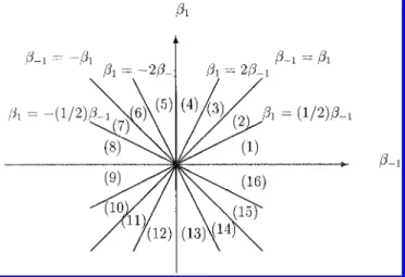
ac-cording to the decreasing (resp. increasing) values of their total-outputs. For example, assume that

(β₋₁, β1) is in the range β−1 > β1 > 0. Then the

elements of ˜B+ are ordered, from the first to

the last, as + + +, + +−, − + +, − + −, since

the total-outputs of these basic patterns are,

re-spectively, β₋₁+ β1, β−1− β1, β1− β−1,−β−1− β1,

which are in an order of decreasing values. In

addi-tion, the elements of ˜B− are ordered, from the first

to the last, as− − −, − − +, + − −, + − +, since

the total-outputs of these patterns are respectively,

−β−1 − β1, β1 − β−1, β−1 − β1, β−1 + β1, which

are in an order of increasing values. Notably, this

ordering depends on the location of (β₋₁, β1) in the

partitioned regions in Fig. 1.

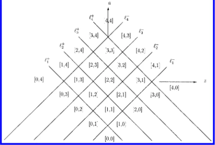
The notations in Fig. 2 are interpreted as

fol-lows. For m, n ∈ I[0, 4], (z, a) ∈ [m, n] means

that B+(A1, z) consists of the first m elements in

˜

B+ _and _B−_(A

1, z) consists of the first n elements

in ˜B−. Notice that the orders of the elements in ˜B+

and ˜B− are dependent on the location of (β₋₁, β1)

in the partitioned regions in Fig. 1. The equations

of the lines in Fig. 2 are given by `+_k : a+z = 1+c+_k,

`−_k : a− z = 1+ c−_k, where c+_k (resp. c−_k) is the

total-Fig. 1. Primary partition of (β−1, β1)-plane.

Fig. 2. Partition of (z, a)-plane for given β₋₁6= 0, β1 6= 0, β−16= ±β1.

output of the (5− k)-th elements in ˜B+ (resp. the

kth element in ˜B−).

If the zero Dirichlet boundary condition (D0

-B.C.) is considered, the patterns +e, or−e, e = “+”

or “−”, at the sites {1, 2} and w+, or w−, w = “+”

or “− ”, at the sites {n − 1, n} will be bordered by

zero, the prescribed data. Hence, the following pat-terns need to be considered,

0| ++ , 0| +− , ++ |0 , −+ |0 ,

0| −− , 0| −+ , +− |0 , −− |0 .

We define the total-output for each of these 1× 3

patterns as the total-output for the “+” or “−” at

its central site. The latter one is given by

Defini-tion 2.1. These 1× 3 patterns may now be ordered

according to their total-outputs. Let ˜ B+ 0 ={0| +e, w+ |0 : w, e = “ + ” or “ − ”} (6) ˜ B− 0 ={0| −e, w− |0 : w, e = “ + ” or “ − ”} . (7)

The elements in ˜B₀+ (resp. ˜B₀−) will be ordered

ac-cording to the decreasing (resp. increasing) values of their total-outputs. Let us take the parameters

(β₋₁, β1) in the region β−1 > β1 > 0 for an

il-lustration. The elements of ˜B₀+ are ordered, from

the first to the last, as ++|0, 0|++, 0|+−, −+|0,

since the total-outputs of these basic patterns are,

respectively, β₋₁, β1,−β1,−β−1. Moreover, the

el-ements of ˜B₀−are ordered, from the first to the last,

as−−|0, 0|−−, 0|−+, +−|0, since the total-outputs

of these patterns are respectively, −β₋₁, −β1, β1,

β₋₁.

For the D0-B.C., to classify the existence of

the boundary patterns in (6), (7) with respect to

(5)

Fig. 3. Further partition of (β₋₁, β1)-plane for the D0 boundary condition.

parameters, the parameter space requires further

partitioning. Firstly, the (β₋₁, β1)-plane is

parti-tioned, as shown in Fig. 3, to determine the

order-ing for total-outputs of the elements in ˜B+∪ ˜B₀+and

the ones in ˜B−∪ ˜B₀−. Consequently, for (β₋₁, β1) in

each of the regions in Fig. 3, the set of feasible basic

patterns, B(A1, z), and the set of feasible

bound-ary patterns, B0(A1, z) = B+0(A1, z)∪ B0−(A1, z),

can be determined and classified with respect to the parameters (z, a). Accordingly, finer partition-ing is performed for the (z, a)-plane, as shown in Fig. 4. The equations of these new separating lines

in Fig. 4 are given by `+_0,k : a + z = 1 + c+_0,k,

`−_0,k: a− z = 1 + c−_0,k, where c+_0,k, c−_0,k are the

total-outputs of the (5− k)-th and the kth elements of

˜

B+

0 and ˜B0−respectively. The feasible boundary

pat-terns (the elements of B0(A1, z)) for parameters in

Fig. 4. Further partition of (z, a)-plane for the D0 bound-ary condition, given β−16= 0, β16= 0, β−16= ±β1.

each partitioned region in Fig. 4 are described as

follows. If (z, a) lies in the region above `+_0,m and

`−_0,k, m, k ∈ I[1, 4], for the largest possible m, k,

then B₀+(A1, z) consists of the first m elements in

(6) and B−₀(A1, z) consists of the first k elements

in (7).

3. Boundary-Pattern and Transition

Matrices

Assume that z and the parameters in the 1×3

tem-plate A1 = [β−1 a β1] are given. The set of basic

patternsB(A1, z) for (1) with these parameters can

then be determined as in Sec. 2. Taking the follow-ing identifications between the indices and the four

1× 2 patterns:

1↔ ++, 2 ↔ +−, 3 ↔ −+, 4 ↔ −− , (8)

we consider the transition matrix M ,

M =       m11 m12 0 0 0 0 m23 m24 m31 m32 0 0 0 0 m43 m44       , (9)

where mij = 0 or 1. The formation of basic

pat-terns can be described as follows: the (i, j)-entry

of M is one if and only if the jth 1× 2 pattern in

(8) can be joined, with one site overlapped, to the

right of the ith 1× 2 pattern in (8) to form a 1 × 3

basic pattern inB(A1, z).

The transition matrix thus formulated can be used to generate patterns on lattices of larger size (of length greater than three). For example, the

(1, 2)-entry of M2, which is in fact m11m12, gives

the number of patterns (yk, yk+1, yk+2, yk+3) =

(+, +, +, −) on a 1 × 4 lattice (let us take k + 1,

k + 2 ∈ Tn\b). The existence of this pattern

indi-cates that there exists (xk, xk+1, xk+2, xk+3)∈ R4

with xk, xk+1, xk+2 > 1 and xk+3 < −1 such

that the stationary equation of (1) is satisfied for

i = k + 1, k + 2. Subsequently, it can be

de-duced that the sum of entries of Mn−2 gives the

number of patterns on Tn. Each of these patterns

y = (y1, y2, . . . , yn−1, yn) ensures the existence of

x = (x1, x2, . . . , xn−1, xn)∈ Rnwith xi > 1 if yi =

“+” and xi <−1 if yi = “−”. Moreover, x satisfies

the stationary equation of (1) for i∈ I[2, n−1]. To

determine if y (resp. x) is indeed a mosaic pattern

(resp. mosaic solution) on Tn, it suffices to check if

y1, y2 and yn₋₁, yn match the boundary condition.

(6)

This task can be resolved by observing further prop-erty of the transition matrices. Indeed, the (i,

j)-entry of Mn−2 gives the number of patterns on Tn

with the ith 1× 2 pattern in (8) at the two sites to

the far left of Tnand the jth 1× 2 pattern in (8) at

the two sites to the far right of Tn. For instance, the

(2, 4)-entry of Mn−2 gives the number of patterns

on Tn with the left-hand side having “+−” and the

right-hand side having “−−”, that is, patterns of

the following form,

+− · · · − − . (10)

This information and our formulation of basic terns allow us to count the number of mosaic

pat-terns on Tn with any boundary condition

men-tioned in Sec. 1. We shall describe the feasible

patterns on the boundary sites with respect to the imposed B.C. also by a matrix, called

boundary-pattern matrix. Let us describe these matrices

MN, MP, MDcorresponding to the Neumann,

peri-odic, and Dirichlet boundary condition respectively. Set MB=       b11 b12 b13 b14 b21 b22 b23 b24 b31 b32 b33 b34 b41 b42 b43 b44       , (11)

where B = N, P, D1, D0. We take (10) as an exam-ple to explain the construction of MB. That is, we consider the following situation:

w +− · · · − − e . (12)

If B = N, for the pattern in (10) to satisfy the Neumann B.C., w and e in (12) have to be w = “+”,

e = “− ”. That is, + + − and − − − have to be

feasible basic patterns (elements of B(A1, z)). If

this is the case, then (MN)24 = b24= 1, otherwise,

(MN)24= b24= 0. For the pattern in (10) to satisfy

the periodic B.C., w and e in (12) have to be w = yn,

e = y1, that is, w = “− ”, e = “+ ”. Thus, if − + −

and − − + are feasible, then (MP)24 = b24 = 1,

otherwise, (MP)24 = b24 = 0. If B = D1, that is,

the Dirichlet B.C. with saturated prescribed data, similar results can be derived. The entries of MB

can thus be obtained as follows. If B = N,

b11= m211 b12= m11m24 b13= m11m31 b14= m11m44 b21= m12m11 b22= m12m24 b23= m12m31 b24= m12m44 b31= m43m11 b32= m43m24 b33= m43m31 b34= m43m44 b41= m44m11 b42= m44m24 b43= m44m31 b44= m2₄₄. (13) If B = P, b11= m2₁₁ b12= m23m31 b13= m31m11 b14= m43m31 b21= m11m12 b22= m23m32 b23= m31m12 b24= m43m32 b31= m12m23 b32= m24m43 b33= m32m23 b34= m44m43 b41= m12m24 b42= m24m44 b43= m32m24 b44= m244. (14)

In fact, (MP)ij = (M2)ji. If B = D1 with ˜y0 =

˜ yn+1= “ + ”, then b11= m2₁₁ b12= m11m23 b13= m11m31 b14= m11m43 b21= m12m11 b22= m12m23 b23= m12m31 b24= m12m43 b31= m23m11 b32= m23m23 b33= m23m31 b34= m23m43 b41= m24m11 b42= m24m23 b43= m24m31 b44= m24m43. (15)

If B = D0, thenB0(A1, z) consists of the 1× 2

pat-terns in (8) which can be bordered by 0 from the

left or from the right. Accordingly, (MD0)ij = 1

if and only if the ith pattern in (8) can be bor-dered by 0 from the left and the jth pattern in (8) can be bordered by 0 from the right. For example,

(MD0)23= 1 if and only if (16) is feasible.

0|+−, −+|0 . (16)

The following main theorem of this presen-tation focuses on CNN with the above-discussed

1 × 3 template. Extension to more general

one-dimensional templates follows from suitable formu-lations on the corresponding transition matrix and

boundary-pattern matrix. The case of the 1× 5

template will be sketched in the next section.

Theorem 3.1. Consider CNN on Tn with

tem-plate A1 = [β₋₁ a β1]. The total number of

(7)

mosaic patterns on Tnsatisfying boundary condition B, B = P, N, D1, D0 is given by 4 X i,j=1 (MB)ij(Mn−2)ij, (17)

where M, MB are as described in (9), (11), (13)–

(15).

As an illustration, exact numbers of moasic pat-terns resulting from computations of (17) for some parameter regions of Figs. 1–4 are presented in the following tables. Table 1 concerns itself with the Neumann and periodic boundary conditions for pa-rameters in regions of Figs. 1 and 2. Table 2 is concerned with the zero Dirichlet boundary condi-tion for parameters in regions of Figs. 3 and 4. In

the tables, Γ1(n) = [(1 + √ 5/2)n+ (1−√5/2)n] + 2 cos[(2π/3)n], Γ2(n) = (2/ √ 5)[(1 +√5/2)n+1 − (1−√5/2)n+1]. In Table 2, [3, 3]1 (resp. [3, 3]2)

represents the subregion of [3, 3], which lies above

(resp. below) `+_0,4 and `−_0,4, while [2, 2]1 represents

the subregion of [2, 2], which lies above `+_0,3and `−_0,3.

Note that there is a symmetry between the feasible patterns and the corresponding parameter regions, cf. [Shih, 1998]. The symmetry results in identical number of patterns for some parameter regions, as shown in the first columns of the tables.

We shall only illustrate the computations for three cases, one for each type of boundary condition.

Table 1. Exact number of mosaic patterns for CNN with the Neumann and periodic boundary conditions.

Region in Regions in

(β₋₁, β1)-plane (z, a)-plane Neumann Periodic (I), (II) [4, 4] [3, 3] [2, 2] 2n Γ2(n) 2 2n Γ1(n) 2 (III), (VIII) [4, 4] [3, 3] [2, 2] 2n 2 0 2n 3 + (−1)n 2 (IV), (VII) [4, 4] [3, 3] [2, 2] 2n 2 0 2n 3 + (−1)n 1 + (−1)n (V), (VI) [4, 4] [3, 3] [2, 2] 2n Γ2(n) 2 2n Γ1(n) 1 + (−1)n

Table 2. Exact number of mosaic patterns for CNN with the zero Dirichlet boundary condition.

Region in Regions in

(β₋₁, β1)-plane (z, a)-plane Dirichlet D0

(1), (4) [4, 4] [3, 3]1 [3, 3]2 [2, 2]1 2n Γ2(n + 1) 2 2 (2), (3) [4, 4] [3, 3]1 [3, 3]2 [2, 2]1 2n Γ2(n + 1) Γ2(n) Γ2(n− 1) (5), (16) [4, 4] [3, 3]1 [3, 3]2 [2, 2]1 2n 2n 2 0 (6), (15) [4, 4] [3, 3]1 [3, 3]2 [2, 2]1 2n 2n 0 0 (7), (14) [4, 4] [3, 3]1 [3, 3]2 [2, 2]1 2n 2n 0 0 (8), (13) [4, 4] [3, 3]1 [3, 3]2 [2, 2]1 2n 2n 2 0

(i) Consider (β₋₁, β1) in the region (I) of Fig. 1 and

(z, a) in the region [3, 3] of Fig. 2. The correspond-ing feasible basic patterns are

B+_(A

1, z) ={+ + +, + + −, − + +}

B−_(A

1, z) ={− − −, − − +, + − −} .

It follows that the entries of the transition matrix

(9) are m11= m12= m24= m31= m43= m44= 1,

and mij = 0 for the other i, j ∈ I[1, 4]. Herein,

we only demonstrate the case of Neumann

bound-ary condition. In this case, every entry of MN is

one, as computed from (13). Therefore, the

to-tal number of mosaic patterns on Tn satisfying the

Neumann boundary condition can be computed by (17). It can be calculated, with help from symbolic

(8)

computation of Mathematica software, that 4 X i,j=1 (MN)ij(Mn−2)ij = 2 √ 5   1 + √ 5 2 !n+1 − 1− √ 5 2 !n+1 .

(ii) Consider (β₋₁, β1) in the region (III) of Fig. 1

and (z, a) in the region [3, 3] of Fig. 2. The corre-sponding feasible basic patterns are

B+_{(A1, z) =}_{{− + +, + + +, − + −} (18)}

B−(A1, z) ={+ − −, − − −, + − +} . (19)

Consequently, the entries of the transition matrix

(9) are m11= m23= m24= m31= m32= m44= 1,

and mij = 0 for the other i, j ∈ I[1, 4]. Herein, we

consider the case of a periodic boundary condition.

Following the formula in (14), the entries of MPare

b11= b12 = b13 = b22 = b33 = b42 = b43 = b44 = 1,

and bij = 0 for the other i, j ∈ I[1, 4]. There

are many patterns for the interior cells. However, imposing the periodic boundary condition strongly

limits the number of feasible patterns on Tn. The

total number of mosaic patterns on Tn satisfying

the periodic boundary condition is computed as 4

X

i,j=1

(MP)ij(Mn−2)ij = 3 + (−1)n.

(iii) Consider (β₋₁, β1) in the region (6) of Fig. 3

and (z, a) in the region [3, 3]1 of Fig. 4. The

cor-responding feasible basic patterns are the same as (18) and (19). Therefore, the entries of the

transi-tion matrix (9) are m11 = m23 = m24 = m31 =

m32 = m44 = 1, and mij = 0 for the other

i, j ∈ I[1, 4]. Herein, we consider the case of

zero Dirichlet boundary condition. The following boundary patterns are feasible,

˜

B+

0(A1, z) ={0| ++, ++ |0, −+ |0}

˜

B−0(A1, z) ={0| −+, −− |0, +− |0} .

As a consequence, the entries of MD0 are b1j = 1,

b4j = 1, j ∈ I[1, 4], and bij = 0 for the other

i, j ∈ I[1, 4]. The total number of mosaic patterns

on Tn satisfying the zero Dirichlet boundary

condi-tion is thus 4 X i,j=1 (MD0)ij(M n−2₎ ij = 2n .

4. Formulation for 1

× 5 Template

In this section, we shall extend the formulations of transition matrix and boundary-pattern matrix to

CNN with 1× 5 template. Namely, we consider

r = 2 and the template

A2 = [β₋₂ β₋₁ a β1 β2] .

Herein, the partitioning for the (β₋₂, β₋₁, β1, β2

)-space is performed so that sixteen possible

total-outputs β₋₂± β₋₁ ± β1 ± β2 for a cell can be

or-dered in each partitioned parameter region. With

given β₋₂, β₋₁, β1, β2, the (z, a)-plane can be

par-titioned so that the existence of basic patterns can be determined for each parameter region of (z, a)-plane.

There are 32 possible basic patterns

corre-sponding to template A2; namely, • • • • •, where

• = “ + ” or “ − ”. A 16 × 16 transition matrix

M = [mij] can be formulated to produce mosaic

patterns on Tn from basic patterns. We take the

following identifications between the indices of the

matrix M and the sixteen 1× 4 patterns:

1↔ + + ++ , 2↔ + + +− , 3↔ + + −+ , 4↔ + + −− , 5↔ + − ++ , 6↔ + − +− , 7↔ + − −+ , 8↔ + − −− , 9↔ − + ++ , 10↔ − + +− , 11↔ − + −+ , 12 ↔ − + −− , 13↔ − − ++ , 14↔ − − +− , 15 ↔ − − −+ , 16↔ − − − − . (20)

In the matrix M , the entries mij = 0 or 1 for

i∈ I[1, 8], j = (i+i−1), (i+i), and for i ∈ I[9, 16],

j = (2i− 18 + 1), (2i − 18 + 2). All other entries are

set to zero. The possible nonzero entries are defined

as follows: mij = 1 if and only if attaching the jth

1×4 pattern in (20), with three sites overlapped, to

the right of the ith 1× 4 pattern in (20) constitutes

a feasible 1× 5 basic pattern. Notably, the purpose

of overlapping three sites in the attaching process is to guarantee the feasibility of produced patterns.

The boundary-pattern matrix MB= [bij] is also

a 16× 16 matrix. For example, consider periodic

boundary condition and the following enclosed

pat-tern on Tn,

w2w1 + + + +· · · + + + − e1e2. (21)

In (21), four “+” at the left end corresponds to the

first pattern in (20) and “+ + +−” at the right end

(9)

corresponds to the second pattern in (20).

Accord-ing to analogous settAccord-ing in Sec. 3, b12 = 1 if and

only if w2 = “ + ” = yn₋₁, w1 = “− ” = yn and

e1 = “ + ” = y1, e2 = “ + ” = y2 are allowed as

the neighbors for the cells at{1, 2} and {n − 1, n}

in (21). More precisely, b12= m59m91m23m35. The

detailed formulation is rather straightforward and is omitted. A formula similar to (17) can thus be

derived for CNN with template A2.

References

Chow, S. N. & Mallet-Paret, J. [1995] “Pattern forma-tion and spatial chaos in lattice dynamical system I,” IEEE Trans. Circuits Syst. 42, 746–751.

Chow, S. N., Mallet-Paret, J. & Van Vleck, E. S. [1996] “Pattern formation and spatial chaos in spatially dis-crete evolution equations,” Rand. Comput. Dyn. 4, 109–178.

Chua, L. O. & Yang, L. [1988a] “Cellular neural networks: Theory,” IEEE Trans. Circuits Syst. 35, 1257–1272.

Chua, L. O. & Yang, L. [1988b] “Cellular neural net-works: Applications,” IEEE Trans. Circuits Syst. 35, 1273–1290.

Chua, L. O. [1998] CNN: A Paradigm for Complexity, World Scientific Series on Nonlinear Science, Series A, Vol. 31 (World Scientific, Singapore).

Hsu, C. H., Juang, J., Lin, S. S. & Lin, W. W. [2000] “Cellular neural network: Local patterns for gen-eral template,” Int. J. Bifurcation and Chaos 10(7), 1645–1659.

Juang, J. & Lin, S. S. [1997] “Cellular neural networks II: Defect pattern and spatial chaos,” preprint. Juang, J. & Lin, S. S. [2000] “Cellular neural networks

I: Mosaic pattern and spatial chaos,” SIAM J. Appl. Math 60(3), 891–915.

Lin, S. S. & Shih, C. W. [1999] “Complete stability for standard cellular neural networks,” Int. J. Bifurcation and Chaos 9(5), 909–918.

Lin, S. S. & Yang, C. S. [2000] “Spatial entropy of 1-dimensional cellular neural network,” Int. J. Bifurca-tion and Chaos 10(9), 2129–2141.

Robinson, C. [1995] Dynamical Systems (CRC Press, Boca Raton, FL).

Shih, C. W. [1998] “Pattern formation and spatial chaos for cellular neural network with asymmet-ric templates,” Int. J. Bifurcation and Chaos 8(10), 1907–1936.

Shih, C. W. [2000] “Influence of boundary conditions on pattern formation and spatial chaos for lattice sys-tems,” SIAM J. Appl. Math. 61(1), 335–368.

Thiran, P. [1993] “Influence of boundary conditions on the behavior of cellular neural networks,” IEEE Trans. Circuits Syst. I: Fundamental Th. Appl. 40(3), 207–212.

Thiran, P., Crounse, K. R., Chua, L. O. & Hasler, M. [1995] “Pattern formation properties of autonomous cellular neural networks,” IEEE Trans. Circuit Syst. 42, 757–774.

Thiran, P., Setti, G. & Hasler, M. [1998] “An approach to information propagation in 1-D cellular nueral net-work — Part I: Local diffusion,” IEEE Trans. Circuit Syst. 45, 777–789.

(10)

1. Jung-Chao Ban. 2014. Neural network equations and symbolic dynamics. International Journal of Machine Learning and Cybernetics . [CrossRef]

2. Jung-Chao Ban, Chih-Hung Chang. 2013. Inhomogeneous lattice dynamical systems and the boundary effect. Boundary Value Problems 2013:1, 249. [CrossRef]

3. WEN-GUEI HU, SONG-SUN LIN. 2009. ZETA FUNCTIONS FOR HIGHER-DIMENSIONAL SHIFTS OF FINITE TYPE. International Journal of Bifurcation and Chaos 19:11, 3671-3689. [Abstract] [References] [PDF] [PDF Plus]

4. JUNG-CHAO BAN, CHIH-HUNG CHANG. 2008. ON THE DENSE ENTROPY OF TWO-DIMENSIONAL INHOMOGENEOUS CELLULAR NEURAL NETWORKS. International Journal of Bifurcation and Chaos 18:11, 3221-3231. [Abstract] [References] [PDF] [PDF Plus]

5. SONG-SUN LIN, WEN-WEI LIN, TING-HUI YANG. 2004. BIFURCATIONS AND CHAOS IN TWO-CELL CELLULAR NEURAL NETWORKS WITH PERIODIC INPUTS. International Journal of Bifurcation and Chaos 14:09, 3179-3204. [Abstract] [References] [PDF] [PDF Plus]

6. CHIH-WEN SHIH, CHIH-WEN WENG. 2002. ON THE TEMPLATES CORRESPONDING TO CYCLE-SYMMETRIC CONNECTIVITY IN CELLULAR NEURAL NETWORKS. International Journal of Bifurcation and Chaos 12:12, 2957-2966. [Abstract] [References] [PDF] [PDF Plus]