RANDOMIZED POLICY OF A POISSON INPUT QUEUE WITH J VACATIONS

(1)

RANDOMIZED POLICY OF A POISSON INPUT QUEUE WITH J

VACATIONS

Jau-Chuan KE1_Kai-Bin_HUANG2 _{Wen Lea PEARN} 2

1_{Department of Applied Statistic, National Taichung Institute of Technology, Taichung 404, Taiwan, China}

[email protected] ( )

2_{Department of Industrial and Engineering Management, National Chiao Tung University, Hsing Chu 300, Taiwan,}

China

[email protected] [email protected]

Abstract

This paper studies the operating characteristics of an M/G/1 queuing system with a randomized control policy and at most J vacations. After all the customers are served in the queue exhaustively, the server immediately takes at most J vacations repeatedly until at least N customers are waiting for service in the queue upon returning from a vacation. If the number of arrivals does not reach N

by the end of the _Jth_{vacation, the server remains idle in the system until the number of arrivals in}

the queue reaches N. If the number of customers in the queue is exactly accumulated N since the server remains idle or returns from vacation, the server is activated for services with probabilitypand deactivated with probability (1−p). For such variant vacation model, other important system characteristics are derived, such as the expected number of customers, the expected length of the busy and idle period, and etc. Following the construction of the expected cost function per unit time, an efficient and fast procedure is developed for searching the joint optimum thresholds (N J∗, ∗) that minimize the cost function. Some numerical examples are also presented.

Keywords: Cost, < , >p N -policy, supplementary variable technique, vacation

1. Introduction

We consider an M/G/1 queuing system in which the server operates a randomized N

policy with at most J vacations. The server leaves for a vacation when the system becomes empty. When the server returns from the vacation, he/she follows a < , >p N operating policy and decides to take another vacation, to remain dormant in the system or to provide

service for the waiting customers. An operating policy is a < , >p N -policy if it prescribes the following four conditions: (i) the server is deactivated when the system becomes empty, (ii) the server is activated (turned on) if there are more than N (N ≥1) customers present in the system, (iii) the number of customers in the system reaches N after the server is deactivated, the server is activated with probability p and

(2)

deactivated with probability 1 p− , and (iv) the server is not activated/deactivated at other epochs. In such policy, the server is activated and keeps serving customers until the system becomes empty. (see Feinberg & Kim 1996)

The modeling analysis for the vacation queuing models has been done by a considerable amount of work in the past and successfully used in various applied problems such as production/inventory systems, communication systems, computer networks and etc. (see survey paper by Doshi, 1986). A comprehensive and excellent study on the vacation models can be found in Levy & Yechiali (1975) and Takagi (1991). Baba (1986) study the M[x]_{/G/1 queuing}

model with vacation time. The first study of vacation models with N policy was done by Kella (1989). The variations and extensions of these vacation models with N policy can be referred to Lee et al. (1994, 1995), Ke (2001), Arumuganathan & Jeyakumar (2005), Moreno (2008), and others. The developments and applications on the optimal control of queuing systems are rich and varied (see Tadj & Choudhury 2005). Moreover, Takagi (1991) first proposed the concept of a variant vacation (a generalization of the multiple and single vacation) for the single arrival M/G/1 regular system. Zhang & Tian (2001) treated the discrete time Geo/G/1 system with variant vacations, where the server will take a random maximum number of vacations after serving all customers in the system. Ke & Chu (2006) examined the variant policy for an M[x]_{/G/1 queuing system by}

stochastic decomposition property. Ke (2007) used supplementary variable technique to study an M[x]_{/G/1 queuing system with balking under a}

variant vacation. Recently, Wang & Huang

(2009) used a maximum entropy approach to examine the steady-state results for the

p N

< , >-policy M/G/1 queue with a unreliable server.

So far very few authors have studied the comparable work on the variant vacation policy for queuing models with N policy, in which the server may take a sequence of finite vacations in the idle time and apply a randomized control policy. This motivates us to develop the variant vacation policy for an M/G/1 queuing system, where the server operates a randomized N policy and takes at most J

vacations when the system is empty. Conveniently, we represent this variant vacation system as M/G/1/VAC ( )J -randomized N

policy queuing model.

The objectives of this paper are as follows: Firstly, we develop the probability generating function of the number of customers present in the system. Secondly, we also derive the busy and idle distributions of the classical N policy with at most J vacations. Through these results and convex property, the expected busy and idle period of our model presented in this paper are obtained. Thirdly, we develop a long-run expected cost function per unit time and then to research the joint optimal threshold values (N J∗, ∗) and we also present a extensive numerical illustration. Finally, some conclusions are drawn.

2. The System

Consider an M/G/1 system in which the server operates a randomized N policy and takes at most J vacations when he finishes serving all customers in the system. The detailed description of the model is given as follows:

(3)

Customers arrive according to a Poisson process with rate λ. The service time provided by a single server is an independent and identically distributed random variable ( )S

with distribution function S t( ) and Laplace-Stieltjes transform (LST) S∗( )θ . Arriving customers who join the system form a single waiting line based on the order of their arrivals; that is, they are queued according to the first-come, first-served (FCFS) discipline. The server can serve only one customer at a time, and that the service is independent of the arrival of the customers. If the server is busy or on vacation, arrivals in the queue must wait until the server is available. Whenever the system becomes empty, the server deactivates and leaves for a vacation with random length V. Once returning from the vacation, the server inspects the system and decides whether to take another vacation, to stay dormant in the system or to resume serving the customers exhaustively. If the number of customers waiting in the queue is less than N when the server returns from the vacation, the server leaves for another vacation with the same length. This pattern continues until at least N customers are found in the queue upon returning from a vacation. However, if the number of customers does not exceed N

by the end of the Jth vacation, the server stays in the system until N customers are accumulated in the queue. If there are N

customers exactly present in the waiting line for service when the server returns from a vacation or the server stays dormant in the system, the server immediately applies a < , >p N -policy listed above. If more than N customers present in the queue upon returning from vacation, the server immediately starts serving the waiting

customers until the system becomes empty. The vacation time V has distribution function

( )

V x and Laplace-Stieltjes transform (LST) ( ).

V∗ θ Furthermore, various stochastic processes involved in the system are independent of each other.

Our model can be applied to many real world systems. In particular, some stochastic production and inventory control systems with a multi-purpose production facility can be effectively studied using such a vacation queuing model. In such systems, the demand for the product is random and can be modeled as a Poisson process. The production time of each unit of the product is a random variable with a general distribution. The production facility performs other tasks utilizing the time between review. An example of Production-To-Stock is considered for illustrative purpose based on Kuo et al. (2009), which it is a production policy in production planning and management. The advantage of Production-To-Stock in comparison with Production-To-Order is that we can improve the service of customers by reducing the waiting times, however, this leads to increase extra costs (keeping stock). Thus it is a important topic how to decide the important parameters to achieve the minimum expected cost. In such an example, it assumed that customer orders for this product arrive according to a Poisson process with rate λ. The system creates an empty slot in the warehouse when an order presents (i.e., an arriving order can be viewed as a slot). When the inventory level is above the reorder point (safe stock) or the number of empty slots is less than N , the production facility stops major production and is available to perform optional jobs j

(4)

(j= , ,...,1 2 J). The optional jobs can be referred to other second tasks or a sequence of finite maintenance policy. On the other hand, if the number of slots reaches N at a vacation completion instant, the production facility may be either set up to replenish the inventory level (to the Order-Up-to-Level) or forced to wait the next orders. Noted that the maximum inventory level (denoted by S ) is greater than the threshold N. Such inventory system (p, ,s S) policy is more flexible and efficient than ordinary (s S, ) inventory policy, where s represents the reorder point and S is the Order-Up-To-Level. One is easy to see that

N = −

s S . Because the demand is random, we can assume that the unmet demand is completely backordered and is supplied after refilling the warehouse. The vacation queuing model presented in this paper is a good approximation of the inventory control system.

3. The Analysis

In this section, we first develop the steady-state differential-difference equations for the variant vacation system by treating the elapsed service time and the elapsed vacation time as supplementary variables. Then we solve these system equations and derive the probability generating functions of various server states at a random epoch.

3.1 System Size Distribution at a Random Epoch

In steady-state, let us assume that S x( ) 0= , for x<0−, S( ) 1∞ = , V x( ) 0= , for x<0 ,−

( ) 1

V ∞ = and these two distribution functions are continuous at x=0, so that

( )

1 ( )

( )x dx dS x_{S x}

μ = ₋ and ω( )x dx=₁dV x₋_{V x}( )_{( )} , where ( )x dx

μ can be interpreted as the conditional probability function of time for completing the service, given that the elapsed time is x and

( )x dx

ω can be referred to the corresponding vacation density.

We define the state of the system at time t

as follows: ( )

Q t ≡ number of customers in the system, ( )

S t− ≡ the elapsed service time, and

( )

j

V t− ≡ the elapsed time of the jth

vacation.

The following random variables we define are used for further development of the variant vacation queuing model:

0, if the server is idle in the system at time , 1, if the server is busy at time ,

2, if the server is on the 1 vacation at ti ( ) th t t t Δ = me ,

1, if the server is on the vacation at time ,

1, if the server is on the th th t j j t J J + + vacation at time .t ⎧ ⎪ ⎪ ⎪ ⎪ ⎪ ⎪ ⎪⎪ ⎨ ⎪ ⎪ ⎪ ⎪ ⎪ ⎪ ⎪ ⎪⎩

Thus the supplementary variables S t−( ) and ( )

j

V t− are introduced in order to obtain a bi-variate Markov process { ( ) ( )}Q t ,δ t , where

( ) 0t

δ = if ( ) 0Δ =t , δ( )t ₌S t−( )_{if ( ) 1}_{Δ =}_t _, and δ( )t =V t_j−( ) if Δ = +( )t j 1

(j= , ,..., .1 2 J)

Furthermore, let us define the following probabilities:

( ) { ( ) ( ) 0}, 0 1 2

n r

(5)

( ) n P x t dx, { ( ) ( ) ( ) ( ) }, r P Q t nδ t S t x S t− − x dx = = , = ; < ≤ + 0 1 x> , ≥ ,n ( ) j n, x t dx Ω , { ( ) ( ) ( ) ( ) }, r j P Q t nδ t V t x V t− − x dx = = , = ; < ≤ + 0 0 1 x> , ≥ , ≤ ≤ .n j J

In steady-state, we can set ( )

n t n

R =lim_→∞R t for 0≤ ≤ −n N 1, and limiting densities P x_n( )=lim_t_→∞P x t_n( , ) for

1,

n≥ and Ω_{j n}_, ( )x =lim_t_→∞Ω_{j n}_, (x t, ) for 0

x> and n≥0, 1≤ ≥j J. According to Cox (1955), the steady-state Kolmogorov forward equations that govern the system can be written as 0 ₀ J0( ) ( ) R x x dx λ =

∫

∞Ω , ω , (1) 1 0 J ( ) ( ) n n n R x x dx R λ =

∫

∞Ω , ω +λ −, 1 2 n= ,...., − ,N (2) 1 ₀ 1 2 1 ( ) ( ) N N N J j j R x x dx R λ ₋ ∞ , ₋ ω λ ₋ = =

∑ ∫

∫

(14)

and the normalization condition 0 0 1 ( ) N n n n n R ∞ ∞P x dx = = +

∑

∑ ∫

N_n₌₀z Rn _n.

Solving the partial differential equations (18) and (19), we obtain (1 ) ( ) (0 )[1 ( )] z x P x z; =P ;z −S x e−λ − . (21) and (1 ) ( ) (0 )[1 ( )] z x, j x z j z V x e−λ − Ω ; = Ω ; − 1 2 . j= , ,...,J (22) Also, solving the differential equation (7) yields

0( ) 0(0)[1 ( )] x 1 2

j, x j, V x e−λ j J

Ω = Ω − , = , ,...,

(23) Now, (23) is multiplied by ω( )x on both sides for j=J and integrating with over x from 0 to ∞, we then have 0 0 0 J ( ) ( ) (0) 0 ( ) x J xω x dx e λ dV x , ∞ _{∞ −} , Ω = Ω

∫

0 0 = (0)ΩJ, α , (24) where α₀=V∗( )λ .

From (1) and (24), it finally yields 0 ,0 0 (0) J R λ α Ω = . (25) Starting with (25) and then solving recursively

(14) through (23) over the range

1 2 1 j= − , − ,...,J J we get on simplification 0 0 ₁ 0 (0) 1 2 1 j _{J j} R j J λ α , _{− +} Ω = , = , ,..., − . (26) Integrating (23) with over x from 0 to ∞

we have 0 0(0) ₀ [1 ( )] x j j V x e λ dx ∞ ₋ , , Ω = Ω

_∫

− 0 0 1 (0)(1 ) j α λ , = Ω − . (27) Using (25)-(27) yields 0 0 0 ₁ 0 (1 ) 1 2 j _{J j} R j J α α , − + − Ω = , = , ,..., . (28) Note that Ω_j_,₀ represents the steady-state probability that there are no customers in the system when the server is on the jth vacation. Let us define Ω₀ the probability that no customers appear in the system when the server is on vacation. Then we have

0 0 0 0 1 ₀ (1 J) J j J j R α α , = − Ω = ∑Ω = . (29) Substituting (21)-(22) into (20) yields

1 (0; ) (0 ) [ (1 )] P z P z S z z λ ∗ = ; − 1 (0 )[ ( (1 )) 1] J j j= z V∗ λ z +∑ Ω ; − − ( )( 1). N R z z λ + − (30) It follows from APPENDIX A that Ω_j(0 );z in (30) can be expressed as 0 0 1 0 0 2 0 , 1 (0 ) 2 3 0 1 2 1 J N n j _{J j} n n R j R z z j J n N λ α λ _α α − = − + ⎧ = ⎪ ⎪ ⎪⎪ Ω ; =⎨ ⎪ ⎪ = , ,..., , = , , ,..., − . ⎪ ⎪⎩

∑

(31)

(7)

where ( ) ( ) ( ) 0 ( ) ( ) n n t t n n n e dV t n V λ λ λ α ∞ − − ∗ λ ! ! =

_∫

= ,

is the probability that n customers arrive during a vacation.

Solving (0 )P ;z from (30), we get 0 (0; ) [ (1 )] zR P z z S z λ λ ∗ = × − − 1 0 1 0 0 0 1 ( (1 )) 1₍₁ ₎ 1 J n N n n J V λ z α _z _α α α ∗ − − = ⎡ ₋ ₋ ₋ ⎢ ₊ ∑ − ⎢⎣ 1 0 ( N n (1 ) N)( 1) n=− z p z z ⎤ + ∑ + − − _⎥⎦. (32) From (21) and (32) yields

0 ( ; ) [ (1 )] zR P x z z S z λ λ ∗ = × − − 1 0 1 0 0 0 1 ( (1 )) 1 (1 ) 1 J n N n n J V z z α λ _α α α ∗ − − = ⎡ ₋ − − ⎢ ₊ _∑ − ⎢ ⎣ 1 0 ( N n (1 ) N)( 1) n=− z p z z ⎤ + ∑ + − − _⎥⎦ (1 ) [1 S x e( )] −λ −z x, × − (33) which leads to 0 ( ) ( ; ) P z =

_∫

∞P x z dx 0 [ (1 )] zR z S z λ λ ∗ = × − − 1 0 1 0 0 0 1 ( (1 )) 1₍₁ ₎ 1 J n N n n J V λ z α _z _α α α ∗ − − = ⎡ ₋ − − ⎢ ₊ _∑ − ⎢ ⎣ 1 0 ( N n (1 ) N)( 1) n=− z p z z ⎤ + ∑ + − − _⎥⎦ ( (1 )) 1 . ( 1) S z z λ λ ∗ ₋ ₋ × ₋ (34) Using (22) and (31) yields

(1 ) 0 1 0 ( ; ) [1 ( )] z x, J R x z λ V x e λ α − − Ω = − (35) and 1 (1 ) 0 2 0 0 ( ; ) N n [1 ( )] z x, j J j n n R x z λ z α V x e λ α − − − − + = Ω =

∑

− 2,3,... .j= J (36) Integrating with over x from 0 to ∞in (35) and (36) respectively, it finally yields

1 0 0 [1 ( (1 ))] ( ) (1 ) J V z z R z λ α ∗ − − Ω = , − (37) and 1 0 0 2 0 [1 ( (1 ))] ( ) (1 ) n N n n j _{J j} V z z z R z λ α α ∗ − = − + − − ∑ Ω = , − 2 3 . j= , ,...J (38) The unknown constant R₀ can be determined by using the normalization condition (15), which is equivalent to 1 (1) (1) J (1) 1 N _j j R +P +

∑

₌ Ω = . Thus we have 0 ₁ ₁ 0 0 0 0 1 1 [ ] ( 1 ) 1 1 J N n J n R E V N p ρ α λ _α α α − − = − = ⎡ ₋ ⎤ + − + ⎢ + ⎥ − ⎢ ⎥ ⎣

∑

⎦ . (39) where ρ λ= E S( ).

Remark 1: In (39), if we let p=1 and N =1, our model becomes the ordinary M/G/1 queuing system with at most J vacations. R₀ can be reduced to 0 0 0 0 1 1 [ ] 1 1 J J R E V ρ α λ α α − = − ₊ −

which agrees with Ke & Chu (2006) Let 1 ( ) _N( ) ( ) J _j( ) j z R z P z z = Φ = + +

∑

Ω be the

probability generating function of the system size distribution at stationary point of time, we then have

(8)

1 1 0 1 0 0 0 0 0 1 1 1 ( 1) [ (1 )] [ (1 )] 1 ( ) (1 ) 1 [ (1 )] J N n n _N n N n J n z z S z V z z z p z R z z S z α _α α λ λ λ α − − ∗ ∗ − = ∗ = ⎛ ⎛ ₋ ⎞ ⎞ + ⎜_⎛ _⎞⎜ ⎟ ⎟ − − − ⎜ − − ⎜ ⎟ ⎟ Φ = ×_⎜⎜_⎜ ⎟_⎟⎜ _⎟+ + − _⎟ − − − _⎜⎝ ⎠_⎜ _⎟ _⎟ ⎜ ⎟ ⎜ _⎝ _⎠ ⎟ ⎝ ⎠

∑

. (40)

It should be noted that the probability generating function given by equation (40) decomposes into two independent random variables: one (the first term) is the system size of the ordinary M/G/1 queue, another (the second term) is the number of customers that arrive during the residual vacation time. Equation (40) can be expressed as following

1 1 0 1 0 0 0 0 1 1 0 0 0 0 1 1 1 [ (1 )] 1 (1 ) 1 (1 )( 1) [ (1 )] ( ) [ (1 )] ( ) 1 ( 1 ) [1 ] 1 J N n n N n N n J n J N n n J n z V z z p z z z S z z z S z E V N p z α _α α λ α ρ λ λ λ α _α α α − − ∗ − = = ∗ ∗ − − = ⎛ ₋ ⎞ + ⎜ ⎟ ⎛ ₋ ₋ ⎞ _⎜ ₋ _⎟ ⋅ + + − ⎜ ⎟ ⎜ ₋ ⎟ ⎜ ⎟ ⎝ _{⎠ ⎜} _⎟ ⎜ ⎟ − − − ⎝ ⎠ Φ = × − − _{+ −} ₊ ₊ − −

∑

. (41)

Remark 2: Suppose that we have p=1 and N=1; then if we put J=1, our model can be simplified to the M G 1/ / queuing system with single vacation. Equation (40) can be rewritten as

(1 )(1 ) [ (1 )] [1 [ (1 )] ( )(1 )] ( ) , [ (1 )] (1 )[ [ ] ( )] z S z V z V z z S z z z E V V ρ λ λ λ λ λ λ ∗ ∗ ∗ ∗ ∗ − − − − − + − Φ = × − − − +

which confirms the result in Section 6 of Choudhury’s system (2002).

3.2 The Expected Number of Customers in the System and the Expected Waiting Time In (40), we evaluate d ( ) |z _z ₁

dzΦ = by using L’hopital rule twice which leads to the expected

number of customers, L_{p N}_, , in the system, given by

1 2 1 0 0 1 0 1 0 0 , 0 0 0 1 1 ( )_[ _] ( )_[1 _] 1 2(1 ) 1 1 J J N N n n p N _J n n R E V E V L ρ λ _ρ α_α nα λ _ρ α_α nα α − − − − = = ⎧ ₋ ₋ ⎪ = + ⎨ ₋ ∑ + ₋ + ₋ ∑ − ⎪⎩ 1 2 2 2 2 0 1 0 0 0 2 2 0 1 ( ) ( )_[1 _] _{[ (} _{1 2 )]} ( )( 1 ) 1 2(1 ) 2(1 ) 2(1 ) J N n n R E V E S α _{N N} _p E S N p _R λ _α λ α ρ ρ ρ − − = ⎫ − ⎪ + − + + ₋ ∑ ⎬+ + − + − − _⎪⎭ − . (42) By using Little’s formula, we can obtain the expected waiting time in the queue, W_{p N}_, , given by

} 1 1 2 0 1 0 1 0 0 0 0 , ₁ 0 1 0 0 0 0 1 1 ( )_[1 _] _{( )[} _] 2 1 1 1 ( ) ( 1 ) [1 ₁ ] J J N N n n n n p N _J J N n n J E V _n _{E V} _n W E V N p α α λ _α _α α α α λ α _α α α − − − − = = − − = − − + ∑ + ∑ − − = ⎧ ₋ ⎫ ⎪ ⎪ + − + + ∑ ⎨ ₋ ⎬ ⎪ ⎪ ⎩ ⎭

(9)

1 2 2 ₂ 2 0 1 0 0 1 1 0 1 0 1 0 0 0 0 0 0 0 1 ( ) ( )_[1 _] ₍ _{1 2 )} ₍ ₎₍ ₁ ₎ 2(1 ) 1 (1 ) 1 1 ( ) ( ) ( 1 ) [1 ] 2 ( 1 ) [1 ] 1 1 J N n n J J J N N n n n n J J E S E V _{N N} _p _{E S} _N _p E V E V N p N p α λ _α _λ ρ α ρ α α λ λ α _α α λ _α α α α − − = − − ⎧ ⎫ ⎪ − ⎪ − ⎨ ₌ ⎬ ₌ ⎪ ⎪ ⎩ ⎭ − + ∑ + − + + − − − − + + ⎧ ⎫ − ⎪ − ⎪ + − + + ₋ ∑ ⎨ + − + + ₋ ∑ ⎬ ⎪ ⎪ ⎩ ⎭ . (43)

Remark 3: Letting p=1, N=1, and J =1, our model can be reduced to the ordinary M/G/1 queuing system with single vacation. Eq. (43) can be reexpressed as:

2 2 ( ) ( ) 2(1 ) 2[ ( ) ( )] p N E V E S W E V V λ λ ρ λ λ , = _∗ + ₋ , +

which is in accordance with Takagi’s system (1991, Section 2.2, p.126).

4. Other System Characteristics

First, we derive the expected length of the busy period, the idle period and the busy cycle for the N -policy M/G/1 queue with at most J vacations. Using the fact that the system characteristics for a < , >p N -policy is a convex combination of the system characteristics for an

N-policy and the system characteristics for an ( N+1)-policy, one can obtain the expected length of the busy period, the idle period and the busy cycle for the < , >p N -policy M/G/1 queue with at most J vacations.

4.1 The Expected Length of the Busy Period

Let 0

N J

Q

, be the number of customers in the

queue at a busy period initiation point (or idle period termination point) for the M/G/1 queuing systems, in which the server operates a

N-policy and takes at most J vacations at the end of each service period.

By conditioning on the number of customers that arrive during a vacation, we have

− = ⋅ − with 1 1 1J 0J 1 B ₌C α −α 1 2 2 2 1J 0J 2 2J 0J 1 B ₌C α −α ₊C α α− 1 2 3 3 3 1J 0J 3 2J 0J 2 1 2 3J 0J 1 B ₌C α −α ₊C α − α α ₊C α α− 1 2 1 1 2 1 2 1 2 1 1 0 1 2 0 1 J 1 J J J J J N N k k k k k k N k k k N B C α −α C α − α α α α − − + = − + + = − = +

∑

+ +

∑

where π_n is the probability that the system state visits n customers during an idle period without vacation.

Remark 4: Using (1)-(3), the following relation of R_n, π_n and α_n is given by 0 0 0 1 n n R R =_α ϕ , ≤ ≤ − ,n N where ϕ_n =

∑

n_i₌₀π α_{i n i}− . Remark 5: Letting J=1, we have A_N_,₁( ) 0z = and

∑

− Then we have 1 0 ,1 0 ( ) ( ) ( 1)N j N j j Q z α z z −ϕ z = = + −

∑

where ϕ₀=α₀, ϕ_n =

∑

_in₌₀π α_{i n i}₋ , π =₀ 1, which agrees with Lee et al. (1995).

₌ ₋_α β −, β = .

In this case, Q_{N J}0_, ( )z can be simplified as 1 0 0 1 0 0 ( ( ) 1) ( ) lim Q ( ) 1 1 N i i i N,J J z z z z α β α α α α − = →∞ − − = + − −

∑

1 0 0 0 0 ( ( ) 1)( 1) ( ) 1 1 N i i i z z z α β α α α α − = − − − = + − −

∑

1 0 0 ( ) 1 1 , 1 N i i i z z α _β α − = − = + −

∑

which agrees with Lee et al. (1994). From (46), the first moment of 0

N J

Q _, can be easily obtained by differentiations, given by

, , 0 , 0 ₀ [ ] (1) (1) [ ] [ ] ( ) 1 ₁ N J N J N J _J E V A B E V E Q λ _α λ α + = ₋ + . − (47)

It is well known that the LST of the busy period started with one customer in the ordinary M/G/1 queuing system queue can be expressed by

( ) [ ( )]

(13)

Following the results by Takagi (1991), the LST of the busy period in the N-policy M/G/1 model with J vacations, denoted by B_{N J}∗_, ( )θ _{, is}

given by B∗_{N J}_, ( )θ =Q_{N J}0_, (B∗( )),θ which implies the expected length of the busy period given by , [ ] [ ] [ ] 1 N J E X E S E B ρ = − , , 0 0 [ ] (1) (1) [ ] 1 1 N J N J J E V A B E V λ λ α α ⎛ ⋅ + ⎞ ×⎜_⎜ + ⎟_⎟ − − ⎝ ⎠. (48)

Remark 7: Letting J→ ∞, it follows from

Remark 6 that we have

1 , 0 0 [ ] [ ] 1 [ ] [ (1 1)] 1 1 N N J i i E S E V E B λ β ρ α − = = + − − −

∑

1 0 0 [ ] = , (1 )(1 ) N i i E V ρ _β ρ α − = − −

∑

which agrees with Lee et al. (1994). 4.2 The Expected Length of the Idle

Period and the Busy Cycle

In this section, we will derive the idle period distribution of the M/G/1 queuing systems, in which the server applies a N-policy and takes at most J vacations at the end of each service period.

Conditioning on the length of the first vacation and size of arrivals during the first vacation, we then have the recursive equation:

, ( , ( ) ) N j I∗ θV ₌x N x ₌k , 1( ), if , if . x N k j x e I k N e k N θ θ θ − ∗ − − − ⎧ _< ⎪ =⎨ ≥ ⎪⎩

After unconditioning on k, we get

(14)

, , 0 0 0 (1) [ ] (1) 1 [ ] 1 1 1 N J N J J J B _{E V} E V A λ α α α = + + − − − , , 0 0 [ ] (1) (1) 1₍ [ ] _). 1 1 N J N J J E V A B E V λ λ λ α α + = + − − (51)

Finally, the expected length of the busy cycle isE I[ _{N J}_, ]+E B[ _{N J}_, ], so from (47) and (50), we can obtain the expected length of the busy cycle

, , , [ _{N J}] [ _{N J}] [ _{N J}] E C =E I +E B , , 0 0 [ ] (1) (1) 1 ₍ [ ] ₎ (1 ) 1 1 N J N J J E V A B E V λ λ λ ρ α α + = + − − − . (52)

4.3 The Expected Length of the Busy Period, the Idle Period and the Busy Cycle for M/G/1/VAC(J) -

Randomized N Policy Queuing Model We denote by (I_N₊₁,B_N₊₁) and

, ,

(I_{p N},B_{p N}) the idle and busy periods for the (N+1)-policy and < , >p N -policy M G/ /1 queue respectively. Also, we let (C_N₊₁,C_{p N}_, ) be a busy cycle for the (N+1)-policy and the

p N

< , >-policy M/G/1 queue, respectively. From Feinberg & Kim (1996), using the property of convex combination and the above formulas (48), (51)-(52) we have , 1 [ _{p N}] [ _N] (1 ) [ _N ] E B = pE B + −p E B ₊ , 1, , 1, 0 0 0 (1) (1 ) (1) (1) (1 ) (1) ( ) 1 = [ ][ ]+ , 1 1 1 1 N J N J N J N J J J pA p A pB p B E S E V λ ρ α α α + + ⎧ _{+ −} _{+ −} ⎫ ⎪ ₊ ⎪ ⎨ ⎬ − ⎪⎩ − − − ⎪⎭ (53) , 1 [ p N] [ N] (1 ) [ N ] E I = pE I + −p E I ₊ , 1, , 1, 0 0 0 (1) (1 ) (1) (1) (1 ) (1) 1 1 = [ ][ ]+ , 1 1 1 N J N J N J N J J J pA p A pB p B E V λ λ α α α + + ⎧ + − + − ⎫ ⎪ ⎪ + ⎨ ⎬ − − − ⎪ ⎪ ⎩ ⎭ (54) , 1 [ _{p N}] [ _N] (1 ) [ _N ] E C =pE C + −p E C ₊ , 1, , 1, 0 0 0 (1) (1 ) (1) (1) (1 ) (1) 1 1 = [ ][ ]+ . (1 ) 1 1 1 N J N J N J N J J J pA p A pB p B E V λ λ ρ α α α + + ⎧ _{+ −} _{+ −} ⎫ ⎪ ₊ ⎪ ⎨ ⎬ − ⎪_⎩ − − − ⎪_⎭ (55)

5. Optimal Policy

In this section, we construct the total expected cost function per customer per unit time for the < , >p N -policy M/G/1 queue with

J vacations, in which N and J are decision variables. Our objective is to determine the optimum joint values of the decision variables

N and J, say N∗ and J∗, so as to minimize the cost function. Let

h

C ≡ holding cost per unit time per customer present in the system;

f

C ≡ cost per unit time for keeping the server off;

o

C ≡ cost per unit time for keeping the server on and in operation;

l

C ≡ setup cost per busy cycle.

Utilizing the definition of each cost element listed above and its corresponding system

(15)

performances, the total expected cost function can be formulated as 0 ( ) ( ) ( ) ( ) ( ) p N p N h p N f o p N p N E I E B F N J C L C C E C E C , , , , , , = + + 1 ( ) l p N C E C _, + (56) Substituting (41), (53), (54) and (55) into (56), we obtain 0( ) 1 h[ J N, p N, ] F N J, =M +C M +M 1 1 0 ₀ ₀ 1 (1) (1 ) (1) (1) (1 ) (1) 1 [ ][₁ ] 1 1 l N J N J N J N J J J C pA p A pB p B E V ρ α , _α + , , _α + , − + _{+ −} _{+ −} , + + − ₋ ₋ (57) where M₁=(C_h+C₀)ρ+C_f(1− ,ρ) 1 2 1 0 0 1 0 1 0 0 , 0 0 0 1 1 ( ) _[ _] ( )_[1 _] (1 ) 1 ) 2(1 ) 1 J J N N n n J N _J n n R E V E V M λ _ρ α_α nα λ _ρ α_α nα α − − − − = = − − = ₋ ₋ ∑ + ₋ + ₋ ∑ 1 2 2 0 1 0 2 0 1 ( ) ( )_[1 _], 1 2(1 ) J N n n E V E S α λ _α α ρ − − = − + + ∑ − − and 2 2 0 , 2 0 ( )( 1 ) [ ( 1 2 )] . 2(1 ) ₂₍₁ ₎ p N R E S N p M _ρ N N p λ R ρ + − = ₋ + − + −

It is easy to see that M₁ in (57) is not a function of the decision variables N and J. Hence, for the determination of the joint optimal thresholds, minimizing (57) is equivalent to minimize

, , ( , ) _h[ _{J N} _{p N}] F N J =C M +M 1 1 0 ₀ ₀ 1 (1) (1 ) (1) (1) (1 ) (1) 1 [ ][₁ ] 1 1 l N J N J N J N J J J C pA p A pB p B E V ρ α , _α + , , _α + , − + _{+ −} _{+ −} + + − ₋ ₋ . (58)

To find the joint optimum values of (N J, ), we should show the existence of convexity or unimodality of F N J( , ). However this is an arduous task to implement because the cost function F

is highly nonlinear. Instead, we will present a procedure that makes it possible to search the joint optimum values (N J∗, ∗).

Let H N J( , )=F N( + , −1 )J F N J( , ). From (58), we then have

, 1 , , 1 ,

( , ) _h[( _{J N} _{J N}) ( _{p N} _{p N})]

(16)

1 2 1 2 0 ₀ 1 (1 ) [ ]( (1) (1 ) (1)) ( (1) (1 ) (1)) [ ] 1 ₁ l N J N J N J N J J C E V pA p A pB p B E V ρ α + , + , _α + , + , ⎧ ⎪ ⎪ + − ⎨ _{+ −} ₊ _{+ −} ⎪ ₊ ⎪ − ₋ ⎩ 1 1 0 ₀ 1 _. [ ]( (1) (1 ) (1)) ( (1) (1 ) (1)) [ ] 1 ₁ N J N J N J N J J E V pA p A pB p B E V α , + , _α , + , ⎫ ⎪ ⎪ − _{+ −} ₊ _{+ −} ⎬ ⎪ + − ₋ ⎪_⎭ (59)

From the definition of the three function M_{J N}_, , M_{p N}_, and A_{N J}_, (1) we have the following corollaries Corollary 1 M_{J N}_, ₊₁−M_{J N}_, ≥ ,0 for N=1, 2,... Corollary 2 M_{p N}_, ₊₁−M_{p N}_, ≥ ,0 for p∈[0,1], N=1, 2,... Corollary 3 1 2 1 2 0 ₀ 1 (1 )( [ ]( (1) (1 ) (1)) ( (1) (1 ) (1)) [ ] 1 ₁ l N J N J N J N J J C E V pA p A pB p B E V ρ α + , + , _α + , + , − _{+ −} ₊ _{+ −} + − ₋ 1 1 0 ₀ 1 _{) 0,} [ ]( (1) (1 ) (1)) ( (1) (1 ) (1)) [ ] 1 ₁ N J N J N J N J J E V pA p A pB p B E V α , + , _α , + , − _{+ −} ₊ _{+ −} ≤ + − ₋ for p∈[0,1], 1, 2,...N = and J=1, 2,3,... For a given value ofJ, the sign of H N J( , ) determines whether F N J( , ) increases or decreases with N. We can conclude that for a given value of J, the optimal value N J∗( ) of

N is given by the first N such that

( ) 0

H N J, > (see Appendix B). That is

{

}

( ) 1 ( ) 0 .

N J∗ =min N≥ |H N J, > (60) Therefore, we can conclude that for each J ,

( )

F N J, has a local minimum value at (N J J∗( ), ∗). From the concept mentioned above, we can locate the minimum value in

( ( ) )

F N J J∗ , ∗ to determine the joint optimal thresholds (N J J∗( ), ∗).

A numerical experiment based on (60) can convince us that the expected cost function is convex. We summarize the procedure to find the joint optimum values of F N J( , ).

Step 1

Set J=1 . Determine N J∗( ) using (60) and compute F N J J( ∗( ) ), using(58).

Step 2

Compute N J∗( +1) using (60) and compute

( ( 1) 1)

F N J∗ + , +J using (58).

Step 3

If F N J( ∗( + , + >1) J 1) F N J J( ∗( ) ), , STOP. The joint optimal thresholds

(N J∗, ∗) (= N J J∗( ) )., Otherwise, GOTO Step 2.

6. Numerical Computations

We present extensive numerical computations to study the effect of various parameters on the optimum joint thresholds of

(17)

To-Stock problem mentioned in Section 2) is

provided to perform the numerical experiments. It is assumed that production time S of customer orders and process time V of the second optional jobs follow 2-stage Erlang distribution and exponential distribution, respectively. The following six parameter settings are considered below: Case 1. λ=0.6,

[ ]

E S =0.2, E V( ) =1.0, C_h =125 , and 1000

l

C = , for different values of p. Case 2. 0 5

p= . , E S( )=0.1, E V( )=1.0, C_h =125, and 500

l

C = , for different values of λ . Case 3. 0 5

p= . , λ =0.6, E V( ) =1.0, C_h =125, and 1000

l

C = , for different service rates (1/E S( )). Case 4. p= .0 5, λ=0.6, E S( )=0.2, C_h =125, and C_l =1000 , for different vacation rates (1/E V( )). Case 5. p= .0 5, λ=0.6, E S( )=0.2,

( )

E V =1, and C_l =1000, for different holding costs. Case 6. p= .0 5 , λ =0.6, E S( ) =0.2,

( )

E V =1, and C_h =150, for different setup costs.

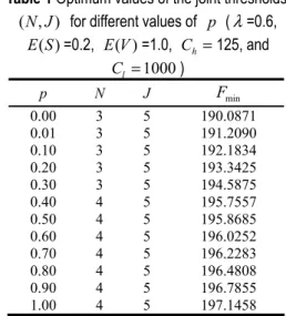
The joint optimum thresholds and the minimum expected cost for the above six parameter cases are summarized in Tables 1-6, respectively. From Table 1 we observe that (i) the minimum expected cost increases as p

increases; and (ii) the optimum N∗ decreases as p decreases. As expected, for a larger N, with a higher probability the production facility replenishes the inventory level to the Order-Up-Level. It means that the facility often replenishes the inventory level due to lower safe-stock/production-point s S= −N . That is, the increase of empty slots frequently causes to replenish the inventory level. In addition, the optimal value of J is always 5 for various values of p, this reveals that the value of p

may not affect the optimum J∗. This implies the optimal number of performing optional jobs

is not affected byp.

Table 1 Optimum values of the joint thresholds

(N J, ) for different values of p (λ=0.6, ( ) E S =0.2, E V( )=1.0, C_h =125, and 1000 l C = ) p N J F_min 0.00 3 5 190.0871 0.01 3 5 191.2090 0.10 3 5 192.1834 0.20 3 5 193.3425 0.30 3 5 194.5875 0.40 4 5 195.7557 0.50 4 5 195.8685 0.60 4 5 196.0252 0.70 4 5 196.2283 0.80 4 5 196.4808 0.90 4 5 196.7855 1.00 4 5 197.1458

Table 2 shows that (i) the optimum N∗

increases with increasing the values of λ; and (ii) the optimum J∗ increases with decreasing the values of λ. It is seen from Table 3 that (i) the minimum expected cost increases as service rate (1/E S( )) increases; and (ii) the optimum

N∗ decreases as service/production rate decreases. It reveals that a larger production rate raises empty slots (i.e., reduces safe-stock).

Moreover, J∗ rarely changes when service rate changes from 1.0 to 10. Intuitively, J∗ seems too insensitive to changes in service rate.

We observe from Table 4 that when vacation rate (1/E V( )) increases from 1.0 to 6.0, N∗

increases from 4 to 5, and then decreases from 5 to 4 when the vacation rate increases from 6.0 to 10.0. The optimum J∗ increases with vacation rate decrease. We can also see that for smaller vacation rate, it tends to have the smaller optimum expected cost. It is reasonable that a larger vacation rate drops the number of performing optional jobs.

(18)

(N J, ) for different arrival rates ( p=0.5, E S( )=0.1, ( ) E V =1.0, C_h =125, and C_l =500) λ N J Fmin 0.01 1 5 45.1405 0.10 1 5 67.9647 1.0 4 5 148.2695 2.0 3 5 164.2802 3.0 4 1 162.0764 4.0 4 1 141.3536 5.0 5 1 123.5126 6.0 5 1 105.8488

(N J, ) for different service rates ( p=0.5, λ=0.6, ( ) E V =1.0, C_h =125, and C_l =1000) 1 ( ) E S N J Fmin 1.0 2 5 123.6220 2.0 3 5 169.9983 3.0 3 5 184.9671 4.0 4 5 192.0016 5.0 4 5 195.8685 6.0 4 5 198.4720 7.0 4 5 200.3432 8.0 4 5 201.7526 9.0 4 5 202.8523 10.0 4 5 203.7342

(N J, ) for different vacation rates (p=0.5, λ=0.6, ( ) E S =0.2, C_h =125, and C_l =1000) 1 ( ) E V N J Fmin 1.0 4 5 195.8685 2.0 4 5 280.8490 3.0 5 5 330.4531 4.0 5 5 364.5354 5.0 5 5 389.5741 6.0 5 5 408.7918 7.0 4 1 423.3651 8.0 4 1 426.4974 9.0 4 1 428.9745 10.0 4 1 430.9825

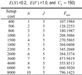
Tables 5-6 shows that (i) the minimum expected cost increases as holding cost (C_h) or setup cost ( )C_l increases; and (ii) N∗

increases as C_h decreases or C_l increases. This reveals that when the holding cost of production faculty increases, the empty slots (N) created by the customers decreases, which is equivalent to raise safe-stock. On the other hand, when the setup cost increases, it presents that the empty slots ( )N created by the customers increases.

(N J, ) for different holding costs ( p=0.5, λ=0.6, ( ) E S =0.2, E V( )=1.0, and C_l =1000) Holding cost N J Fmin 15 11 5 92.1219 20 10 5 101.9221 25 9 5 110.1240 30 8 5 117.2279 35 7 5 123.8267 60 6 5 150.1092 70 5 5 158.3801 100 4 5 180.4089 150 3 5 208.5086 200 2 5 230.8111

(N J, ) for different setup costs (p=0.5, λ=0.6, ( ) E S =0.2, E V( )=1.0, and C_h =150) Setup cost N J Fmin 400 1 5 107.1984 500 2 5 128.2253 800 3 5 180.1987 1000 3 5 208.5086 1500 4 5 270.5865 1800 5 5 304.0408 2200 5 5 345.2048 2600 6 5 384.3374 3600 7 5 473.9419 4600 8 5 555.8513 6000 9 5 660.5020 8000 10 5 796.1423

(19)

It should be noted that J∗ does not change at all when C_h changes from 15 to 200 or C_l

changes from 400 to 10000. The optimum value

J∗ almost does not change in C_h or C_l. Our numerical investigations indicate that (i) λ

significantly affects the optimum value N∗

than p, 1/E S( ), and 1/E V( ), and (ii) λ and 1/E V( ) have a much significant effect on the optimum value J∗ than p and 1/E S( ) do. It is interesting to mention that C_h and C_l may have a much more significant effect on N∗ than the other system parameters.

7. Conclusions

In this paper, we analyzed the system size of the < , >p N -policy M/G/1 queuing system with at most J vacations. A cost model is developed based on some system characteristics derived. Although the convexity or unimodality of the cost function cannot be proved analytically, we present an efficient algorithm to find the joint optimal thresholds. We also perform the extensive numerical computations to study the effect of system parameters on the optimal thresholds (N J∗, ∗) . This research presents an extension of the vacation model theory and the analysis of the model will provide a useful performance evaluation tool for more general situations arising in practical applications, such as production systems, flexible manufacturing systems, computer and communication systems, transportation systems, inventory problems, and many other related systems.

Acknowledgments

The authors would like to thank the anonymous referees and editor for detailed

report on an earlier version of this paper, which contributed significantly to improvement in the presentation of this paper.

Appendix A

Proof of Equation (31)

Proof. From (13) and (26)-(27) we obtain 0 1 0 (0 )z λR_J α Ω ; = . (A1) Solving the differential equation (8) for j=1 and n=1, if finally yields

1 0 0 11 ( ) 1 ( ) ( ) 1 ( ) x x e x dx V x x e V x λ λ λ ∞ , , Ω ∫ ₋ Ω = − 2 0 0 (1 ( )) J x R x V x eλ λ α − = .

It then follows from (14) that we obtain 2 1(0) ₀ 11( ) ( )xω x dx ∞ , , Ω =

∫

Ω 2 0 0 0 0 2 2 0 ( ) ( ) ( ) x J J R xe dV x R dV d λ λ α λ _λ λ λ α ∞ ₋ ∗ − + = = − .

∫

Using the same manner in the rest cases of 2,3,...,

j= J and n=1, 2,...,N−1 we can finally summarize that

0 0 2 0 ( ) (0) n n j n J j n R d n _d λ λ α λ α , _{− +} − Ω = _! 0 2 0 2 3 1 2 3 1 n J j R j J n N λ _α α − + = , = , ,..., , = , , ,..., − . (A2) From (A1)-(A2) and (26), it finally yields

0 0 1 0 _, 0 2 0 , 1 (0 ) 2 3 . J j _N n n n J j R j z _R z j J λ α λ _α α − = − + ⎧ = , ⎪ ⎪ Ω ; =⎨ ⎪ _{= , ,...,} ⎪ ⎩