存貨揭露與銷售及盈餘預測：IFRS與非IFRS之比較 - 政大學術集成

全文

(1)國立政治大學會計學系碩士班碩士論文. 指導教授：. 立. 張清福博士. 政治大. ‧ 國. 學. 存貨揭露與銷售及盈餘預測：IFRS 與非 IFRS 之比較. ‧. DO INVENTORY DISCLOSURES PREDICT SALES AND. y. Nat. n. al. er. io. sit. EARNINGS: IFRS VS. NON-IFRS. Ch. 研究生：. 中. 華. 民. 國. engchi. i n U. v. 陳采薇. 一百零一. 撰. 年. 七. 月.

(2) 致謝詞首先，要感謝指導教授張清福老師。寫作論文的過程，大部分是在國外進行。繁重的課業、時區的差異、資料文獻的限制，使寫作過程頗為曲折。然而，老師對我十分的體諒與包容，以各種方式與我進行即時的溝通，盡其所能的在第一時間解答我的問題。任何問題，老師總是耐心親切的解釋至我完全了解，不僅讓我能夠無所掛慮的詢問和討論任何問題，更有豁然開朗之感。在我鑽牛角尖之際，老師總會適時的關心，把我引回正途，化解我的迷惘與倔強。老師溫良恭謙的學者風範，令學生十分感佩。謝謝老師。. 政治大感謝口試委員李建然教授與許崇源教授。李建然教授細心的閱讀了我的整篇立. ‧ 國. 學. 論文，論文上密麻的記號與折痕令我十分感動。口試時所提出的深入而獨到的見解，提供學生不同的思考機會。許崇源教授一針見血的點出與學生研究高度且直. ‧. 接相關的文獻，令學生的論文更為完整周全。兩位教授的指教，使我獲益良多。. Nat. sit. y. 感謝研究所同學詹竣揚，在研究所生涯中，持續的關心與陪伴。在論文學位. n. al. er. io. 考試之際，每天一通電話詢問是否有需要幫忙的地方，鼎力協助不計回報。感謝. i n U. v. 余安婷、蘇奧迪、葉添得、黃子齡與袁麗芸學妹的幫助，讓我能夠順利的完成論. Ch. engchi. 文、進行口試。我是如此的幸運與幸福，能夠擁有一群真心誠摯的朋友。最後，要感謝我的家人，你們是我的生命中，最珍貴的資產和最堅強的後盾，讓我能以一顆溫暖又安穩的心，無後顧之慮的完成學業。謹將此論文，獻給所有關愛我的人。陳采薇謹誌於政大會計學系研究所中華民國一百零一年七月 I.

(3) 摘要文獻顯示存貨對於銷售和盈餘具有預測能力（Bernard and Noel 1991）。本文進一步探討比較後進先出法和國際會計準則允許之存貨計價方法所揭露之存貨，對於銷售和盈餘之預測能力。2003 年發布之國際會計準則第二號公報「存貨」，禁止公司採用後進先出法衡量存貨，本研究擬觀察後進先出法和非後進先出法存貨對公司銷售與盈餘的預測能力是否有所差異。本研究選取採用後進先出法並且揭露後進先出存貨準備之公司做為樣本，計. 治政大存貨與依國際會計準則揭露之存貨，孰者對銷售與盈餘之預測更具攸關性。實證立. 算出樣本公司在國際會計準則規定下應有之存貨水準，測試與比較後進先出法之. 結果顯示，後進先出存貨與國際會計準則存貨代理變數之實證結果並不顯著，顯. ‧ 國. 學. 示存貨在銷售與盈餘之預測迴歸模型中為一雜訊，存貨對銷售和盈餘之預測並不. ‧. 具有增額資訊，也說明存貨生產平穩理論與避免缺貨理論無法解釋存貨對銷售和. y. Nat. 盈餘預測之關聯性，因此無法判斷採用何種存貨計價方法所揭露之存貨，對銷售. n. al. er. io. sit. 與盈餘較具預測能力。. Ch. engchi. i n U. v. 關鍵詞: 存貨計價方法，國際會計準則第二號公報「存貨」，銷售與盈餘預測. II.

(4) Abstract In economic literature, production smoothing model and stockout model address the predictability of inventory disclosure on sales and earnings. Based on these models, Bernard and Noel (1991) show that inventory disclosure predicts sales and earnings. This study further investigates and compares the predictability of the sales and earnings by inventory reported under last in, last out (LIFO) and that under International Accounting Standard 2 (IAS 2). Thus this study compares the predicting ability of inventory on sales and earnings under IFRS and non-IFRS.. 政治大 This study selects the companies adopting LIFO and disclosing LIFO reserve, 立. calculates the inventory reported under IFRS, and determines the inventory’s ability to. ‧ 國. 學. predict future sales and earnings under different inventory valuation methods. The. ‧. empirical results show that the coefficients for the unexpected inventories under LIFO. sit. y. Nat. and IFRS are both statistically insignificant, suggesting that the unexpected. io. er. inventories are merely noises in the models, and that the effects of production smoothing model and stockout model are not prevailed. Thus, it is difficult to. al. n. v i n C h method can generate determine which inventory valuation the inventory that leads to engchi U better sales and earnings prediction.. Key Words: Inventory valuation method, International Accounting Standard 2, Sales and earnings prediction.. III.

(5) TABLE OF CONTENT Chapter 1 Introduction ........................................................................................................1 1.1 Research Purpose and Motivation ...............................................................................1 1.2 Research Questions .......................................................................................................4 1.3 Research Structure.........................................................................................................5 Chapter 2. Literature Review .............................................................................................6 2.1 The Development and Fundamental Principles of IAS2 .......................................6 2.2 Inventory, Sales and Earnings Related Literature ...................................................10 Chapter 3. Methodology .......................................................................................... 14. 治政 14 3.1 Research Hypotheses ......................................................................................... 大立 3.2 Sample Selection................................................................................................ 18 ‧ 國. 學. 3.3 Research Method ............................................................................................... 21. ‧. 3.4 Empirical models and Variable Description ...................................................... 22 Chapter 4. Empirical Results and Analysis ............................................................. 28. y. Nat. io. sit. 4.1 Descriptive Statistic ........................................................................................... 28. n. al. er. 4.2 Empirical Results ............................................................................................... 30. Ch. i n U. v. Chapter 5. Conclusion ............................................................................................... 41. engchi. Reference .................................................................................................................... 43. IV.

(6) LIST OF TABLES Table 3.1 Sample Selection Criteria ............................................................................ 20 Table 4-1 Descriptive Statistics of Final Prediction Models ....................................... 28 Table 4-2 Basic Sales Prediction Model ...................................................................... 30 Table 4-3 Basic Earnings Prediction Model ................................................................ 31 Table 4-4 Basic Profit Margins Prediction Model ....................................................... 32 Table 4-5 Inventory Expectations Model—LIFO method ........................................... 33 Table 4-6 Inventory Expectations Model—IFRS method ........................................... 35 Table 4-7 Final Sales Prediction Model ....................................................................... 36. 治政 Table 4-8 Final Earnings Prediction Model ................................................................. 38 大立 Table 4-9 Final Profit Margins Prediction Model ........................................................ 39 ‧. ‧ 國. 學. n. er. io. sit. y. Nat. al. Ch. engchi. V. i n U. v.

(7) LIST OF FIGURES Figure 1-1 Research Process and Structure ................................................................... 5. 立. 政治大. ‧. ‧ 國. 學. n. er. io. sit. y. Nat. al. Ch. engchi. VI. i n U. v.

(8) 1. INTRODUCTION 1.1 Research Purpose and Motivation International Financial Reporting Standard (IFRS) convergence has been a current and emerging accounting issue in the United States. International Accounting Standard 2 (IAS 2) provides guidance on the cost formulas that are used to assign costs to inventories and prohibits the use of last in, last out (LIFO) cost formula. However, a lot of American companies adopt LIFO for tax advantage. Consequently, the change would have a significant effect on those companies.. 政治大 Past LIFO research generally focuses on two areas: management’s inventory 立. accounting method decision and investors' reactions to LIFO adoptions. However, few. ‧ 國. 學. literatures consider the underlying economic implication of inventory accounting. ‧. methods and the effect of inventory accounting methods on financial statements. This. sit. y. Nat. study examines how inventory accounting methods affect the presentation of. io. er. inventory, how the inventory affects future sales and earnings, and demonstrates the effect with economic models and empirical study. Accounting methods directly affect. al. n. v i n inventory, and inventory is one C of the key aspects of financial h e n g c h i U statement analysis.. Inventory levels reveal management’s inventory behavior and decisions, imply the historical sales patterns, and can be regarded as one of the indicators of future sales and earnings. IAS 2 prohibits the use of LIFO inventory valuation method, and suggests companies adopt FIFO or weighted average method to measure inventory cost. According to IAS 2, paragraph 25, the cost of inventories, other than those that are not ordinarily interchangeable and goods or services produced and segregated for specific projects, shall be assigned by using the first-in, first-out (FIFO) or weighted average 1.

(9) cost formula. As a result, this study categorized and defined FIFO and weighted average methods as IFRS inventory valuation method. Generally speaking, IFRS inventory valuation method presents physical flow of goods better than LIFO method does. Under LIFO method, the items remaining in inventory are recognized as if they were the oldest, while under IFRS method, the items are recognized at most recent or average cost. As a result, the International Accounting Standards Board (IASB) decided to eliminate the LIFO method because of its lack of representational faithfulness of inventory flows.. 政治大. According to past study, there is a strong connection between inventory and. 立. future sales and earnings. The reason is that inventory reveals information concerning. ‧ 國. 學. a company’s inventory policy and management’s sales decision, so inventory can be one of the leading factors for future sales and earnings. According to the production. ‧. smoothing model, inventory levels reflect management’s expectations about future. y. Nat. io. sit. sales and demand, so inventory should be positively related to future sales. In the. n. al. er. stockout model, lower inventory levels indicate higher frequency of stockouts and a. i n U. v. higher level of demand, so inventory levels may be inversely related to future sales.. Ch. engchi. Abarbanell (1997) indicates that inventory is one of the accounting-based fundamental signals of future earnings and security prices. Thomas (2003) points out that inventory changes represent the one component that exhibits a consistent and substantial relation to future returns. In Gupta’s (2010) research, he finds that inventory overproduction is highly related to a company’s accounting performance and stock returns. All the literatures suggest that inventory is highly related to, and is able to predict future sales and earnings. Recently, sales prediction has become an important issue for a company. An accurate demand and sales prediction can be highly beneficial to a company. Brown 2.

(10) (2009) concludes that improvements in sales forecast accuracy can not only result in fewer quantity adjustments in purchase orders and allow for the factories to stage materials ahead of time, but can also decrease stockout and increase sales. Aror (2011) points out that better sales forecasting can lead to better demand and supply visibility and provide management with information to make better decision and strategies. The purpose of this study is to discuss the inventory’s ability to predict sales and earnings under different accounting methods. This study assumes that inventory has better sales predictive ability if the inventory reflects only volume changes, and under. 政治大 this assumption, inventory 立 reported under LIFO method should be a stronger indicator. LIFO method, inventory changes are mostly affected by the volume changes. With. ‧ 國. 學. of future sales and earnings. This study can provide favorable information and insight for investors to make investment decisions. Thus, the study is also aim at decreasing. ‧. the IFRS convergence difficulties in the United States.. n. er. io. sit. y. Nat. al. Ch. engchi. 3. i n U. v.

(11) 1.2 Research Questions According to the research motivation and the literatures of related study, the research questions of this study are as follows: 1. Are inventories reported under IFRS and LIFO inventory valuation methods positive or negative indicators of future sales and earnings? 2. Is inventory reported under LIFO inventory valuation method a stronger indicator of future sales and earnings than the inventory reported IFRS method?. 立. 政治大. ‧. ‧ 國. 學. n. er. io. sit. y. Nat. al. Ch. engchi. 4. i n U. v.

(12) 1.3 Research Structure The research process and structure is presented as follow:. Figure 1-1. Research Process and Structure. Introduction. 政治大. 立Literature Review. ‧. ‧ 國. 學. n. al. er. io. sit. y. Nat. Research Method. Ch. i. e. i n U. v. h Analysis n g cand Empirical Results. Conclusion. 5.

(13) 2. LITERATURE REVIEW 2.1 The Development and Fundamental Principles of IAS2 International Accounting Standards 2 (IAS 2), ―Valuation and Presentation of Inventories in the Context of the Historical Cost System,‖ was first issued in October 1975 by International Accounting Standards Committee (IASC). In December 1993, IASC issued a revised IAS 2 Inventories. In December 1997, the Standing Interpretations Committee developed SIC-1 ―Consistency-Different Cost Formulas for Inventories.‖ To improve the International Accounting Standards, the. 政治大. International Accounting Standards Board (IASB) revised IAS 2 again in December. 立. 2003, which replaced both IAS Inventories in 1993 and SIC-1. The revised IAS 2 was. ‧ 國. 學. effective and applied annually from January 1, 2005.. ‧. The objective of IAS 2 is to prescribe the accounting treatment for inventories.. sit. y. Nat. It provides guidance for determining the cost of inventories and for subsequently. io. er. recognizing an expense, including any write-down to net realizable value. It also provides guidance on the cost formulas that are used to assign costs to inventories.. n. al. Ch. engchi. i n U. v. The scope of IAS 2 includes assets held for sale in the ordinary course of business (finished goods), assets in the production process for sale in the ordinary course of business (work in process), and materials and supplies that are consumed in production (raw materials). However, IAS 2 excludes certain inventories from its scope, such as work in process arising under construction contracts, financial instruments, biological assets related to agricultural activity, and agricultural produce at the point of harvest. One of the most fundamental principles of IAS 2 is that inventories are required to be stated at the lower of cost and net realizable value (NRV). The inventory cost 6.

(14) should include costs of purchase (including taxes, transport, and handling) net of trade discounts received, costs of conversion (including fixed and variable manufacturing overheads) and other costs incurred in bringing the inventories to their present location and condition. Inventory cost should not include abnormal waste, storage costs, administrative overheads unrelated to production, selling costs, foreign exchange differences arising directly on the recent acquisition of inventories invoiced in a foreign currency, and interest cost when inventories are purchased with deferred settlement terms.. 政治大 estimated cost of completion 立and the estimated costs necessary to make the sale.. NRV is the estimated selling price in the ordinary course of business, less the. ‧ 國. 學. Estimates of net realizable value are based on the most reliable evidence available at the time the estimates are made, of the amount the inventories are expected to realize.. ‧. The amount of any write-down of inventories to net realizable value and all losses of. sit. y. Nat. inventories shall be recognized as an expense in the period the write-down or loss. n. al. er. io. occurs. The amount of any reversal of any write-down of inventories, arising from an. i n U. v. increase in net realizable value, shall be recognized as a reduction in the amount of. Ch. engchi. inventories recognized as an expense in the period in which the reversal occurs. Inventories should be written down to net realizable value item by item. A company can only group similar or related items when the inventory relating to the same product line that have similar purposes or end uses, are produced and marketed in the same geographical area, and cannot be practicably evaluated separately from other items in that product line. It is not appropriate to write inventories down on the basis of a classification of inventory, In terms of techniques for the measurement of cost, standard cost method, retail method, specific costs method, FIFO and weighted average cost method are allowed. 7.

(15) Standard costs take into account normal levels of materials and supplies, labor, efficiency and capacity utilization and should be regularly reviewed and revised in the light of current conditions. Specific costs are attributed to the specific individual items of inventory that are not interchangeable. The retail method is often used in the retail industry and the cost of the inventory is determined by reducing the sales value of the inventory by the appropriate percentage gross margin.. For items that are. interchangeable, IAS 2 allows the FIFO or weighted average cost formulas. The same cost formula should be used for all inventories with similar characteristics as to their. 政治大 The LIFO formula, which 立 had been allowed prior to the 2003 revision of IAS 2,. nature and use to the entity.. ‧ 國. 學. is no longer allowed for several reasons. First, the LIFO method treats the newest items of inventory as being sold first, and consequently the items remaining in. ‧. inventory are recognized as if they were the oldest. Therefore, the use of LIFO results. sit. y. Nat. in inventories being recognized in the balance sheet at amounts that bear little. n. al. er. io. relationship to recent cost levels of inventories. This is generally not a reliable. i n U. v. representation of actual inventory flows. Second, the use of LIFO in financial. Ch. engchi. reporting is often tax-driven, because it results in cost of goods sold expense calculated using the most recent prices being deducted from revenue in the determination of the gross margin. However, IASB indicates that tax considerations do not provide an adequate conceptual basis for selecting an appropriate accounting treatment and that it is not acceptable to allow an inferior accounting treatment purely because of tax regulations and advantages in particular jurisdictions. In addition, it is not appropriate to allow an approach that results in a measurement of profit or loss for the period that is inconsistent with the measurement of inventories for balance sheet purposes. As a result, IASB decided to eliminate the LIFO method because of its lack 8.

(16) of representational faithfulness of inventory flows. IAS 2 covers the cost of inventories of a service provider. To the extent that service providers have inventories, they measure them at the costs of their production. These costs consist primarily of the labor and other costs of personnel directly engaged in providing the service, including supervisory personnel, and attributable overheads. Labor and other costs relating to sales and general administrative personnel are not included but are recognized as expenses in the period in which they are incurred. The cost of inventories of a service provider does not include profit. 政治大. margins or non-attributable overheads that are often factored into prices charged by. 立. service providers.. ‧ 國. 學. IAS 2 also has certain disclosure requirement for inventory. A company must disclose the accounting policy for inventories, the carrying amount, for merchandise,. ‧. supplies, materials, work in progress, and finished goods. The carrying amount of any. y. Nat. io. sit. inventories carried at fair value less costs to sell, the amount of any write-down of. n. al. er. inventories recognized as an expense in the period, the amount of any reversal of a. i n U. v. writedown to NRV and the circumstances that led to such reversal, the carrying. Ch. engchi. amount of inventories pledged as security for liabilities, and cost of inventories recognized as expense.. 9.

(17) 2.2 Inventory, Sales and Earnings Related Literature Broadly speaking, past LIFO research has focused on two key questions. The first question is about the sophistication of managers’ inventory accounting method decision. For example, Bar-Yosef (1992) and Cushing (1992) discuss whether managers would choose LIFO to minimize the company’s tax payment, or they would choose FIFO to avoid lower reported earnings. Hughes, P.J (1994) analyzes the manager's choice of both an inventory accounting method and capital structure in order to communicate private information about the firm's future cash flows.. 政治大. The second question is about investors' reactions to LIFO adoptions. For. 立. example, Biddle (1988) focuses on analysts’ forecast errors and stock price behavior. ‧ 國. 學. near the earnings announcement dates of LIFO adopters. Jennings (1992) examines investor and stock price reaction to LIFO adoption decisions. Kang (1993) discusses. ‧. the stock price effects of LIFO tax benefits. Guenther (1994) analyzes the effect that. y. Nat. io. sit. the ―LIFO reserve‖ has on firm value, and the results indicate a significant negative. n. al. er. relation between the LIFO reserve and the value of equity because larger LIFO. i n U. v. reserves may be associated with greater accounting costs and may be a proxy for the. Ch. engchi. average expected effect of future inflation on the firm’s input prices. However, few literatures consider the effect of inventory accounting methods on financial statements analysis. This study examines how inventory accounting methods affect inventory and how the inventory affects future sales and earnings. According to the IASB, LIFO is generally not a reliable representation of actual inventory flows. International Accounting Standard (IAS) 2 sets out the accounting treatment for inventories and provides guidance on determining their cost. IAS 2 points out that the LIFO method treats the newest items of inventory as being sold 10.

(18) first, and consequently the items remaining in inventory are recognized as if they were the oldest; therefore, the use of LIFO results in inventories being recognized in the balance sheet at amounts that bear little relationship to recent cost levels of inventories. Some respondents argued that the use of LIFO has merit in certain circumstances because it partially adjusts profit or loss for the effects of price changes. However, the Board concluded that it is not appropriate to allow an approach that results in a measurement of profit or loss for the period that is inconsistent with the measurement of inventories for balance sheet purposes. As a result, the Board decided. 政治大 Several studies have addressed 立 that Inventory is one of the fundamental signals. to eliminate the allowed alternative of using the LIFO method.. ‧ 國. 學. for Future Earnings. Chi-Wen Jevons Lee (1988) finds significant association between the Earnings and Profit ratio (E/P ratio) and the inventory accounting methods.. ‧. According to common economic intuition, each dollar of pretax cash flow in a FIFO. sit. y. Nat. firm should lead to higher accounting earnings, higher tax payments and a higher. n. al. er. io. stock price than in a FIFO firm, so the E/P ratios of the FIFO firms should be higher. i n U. v. than those of the LIFO firms. However, Lee finds the E/P ratios of the LIFO firms are. Ch. engchi. higher than those of the FIFO firms. Although he hasn’t established a complete causal link, he shows that inventory accounting can affect a company’s stock valuation. Bernard (1991) examines the relation between inventory disclosures, future sales and future earnings. He uses a ―lead time‖ or ―production smoothing‖ model and a ―stockout model‖ of inventory to evaluate the predictive ability of inventory. He finds that an unexpected change in total inventory is a negative leading indicator of future earnings and profit margins, because an inventory buildup generally reflects decline in future sales, but the increase in inventory is positively related to future sales, because inventory reflects management's private information about demand. This paper 11.

(19) reveals a strong relation between inventory and future sales and earnings, and provides valuable insight that inventory disclosures can improve predictions of future sales and earnings. Thiagarajan. (1993) Abarbanell (1997) analyzes the underlying relations between accounting-based fundamental signals and security prices. He finds that inventory is one of the fundamental signals for future earnings for several reasons. One of the reasons is that increase in finished goods inventory that outstrips sales demand is predicted to indicate bad news for earnings. The other reason is that inventory. 政治大 performance. The study shows 立 that inventory is one of the crucial elements for. changes in excess of sales changes are negatively associated with future earnings. ‧ 國. 學. earnings information analysis.. Thomas and Zhang (2003) indicate that the negative relation between accruals and. ‧. future abnormal returns is due mainly to inventory changes, and inventory changes. y. Nat. io. sit. represent the one component that exhibits a consistent and substantial relation with. n. al. er. future returns. They document several key empirical regularities for extreme. i n U. v. inventory change companies and explore the relation between sales and inventory. Ch. engchi. changes. They think firms with inventory increases experience higher profitability, growth, and stock returns over the prior five years, but those trends reverse after the extreme inventory change. They also think quarterly cost of goods sold (COGS) and sales ratio and selling, general and administrative (SG&A) expenses and sales ratio exhibit similar patterns. In addition, LIFO companies with inventory increases represent one subgroup of extreme inventory change companies that exhibits abnormal return and profitability patterns unlike those observed for other companies. Jennings and Thompson (1996) investigate the relative usefulness of LIFO and non-LIFO financial statements as a basis for valuation. It is often argued that LIFO 12.

(20) income statements are more useful as a basis for valuation than those prepared under alternative cost-flow assumptions because LIFO cost of goods sold is based on relatively current inventory costs. In contrast, non-LIFO balance sheets are alleged to be more useful for valuation because their inventory values better represent the net assets available to generate future resource inflows. Jennings and Thompson use LIFO reserve disclosures to construct ―as if‖ non-LIFO income statements and balance sheets for 991 LIFO users and compare the extent to which elements of actual LIFO financial statements and their ―as if‖ non-LIFO counterparts explain the. 政治大 LIFO cost of goods sold is a more useful indicator of future resource outflows, LIFO 立 observed distribution of equity values for these firms. The comparisons indicate that. reserve disclosures are useful supplements to the LIFO balance sheet, and LIFO-based. ‧ 國. 學. income statements explain slightly more of the cross-sectional variation in equity. ‧. values than their ―as if‖ non-LIFO counterparts.. n. er. io. sit. y. Nat. al. Ch. engchi. 13. i n U. v.

(21) 3. METHODOLOGY In this chapter, Section One will develop the hypotheses for this study, which are based on two economic models. Section Two will present the data selection process. Section Three will discuss the research methodology and design, and Section Four will examine the empirical models and variables.. 3.1 Research Hypotheses 3.1.1 The Production Smoothing Model. 政治大 inventory in economic literature 立 (Blinder 1986). A necessary motive for a company to The production smoothing model is one of the most widely studied models of. ‧ 國. 學. smooth production is that demand varies through time. If there is a random element to demand, a company may decide to smooth production and treat inventories as a buffer. ‧. stock. Therefore, a firm is said to smooth production if the variance of production is. io. sit. y. Nat. less than the variance of sales.. n. al. er. The information structure of the production smoothing model presumes that both. i n U. v. cost shock and demand shock would affect production decisions. According to Guido. Ch. engchi. Lorenzoni (2006), demand shock is a sudden event that causes a shift in consumer expectations, which increases or decreases demand for goods or services temporarily, while cost shock is an event that causes a sudden increase of decrease of production costs. The production smoothing model assumes that managers can observe cost shock and part of demand shock before choosing its level of production, price, and expected sales. After these decisions are made, the rest of the demand shock is observed and actual sales are determined. The inventory levels for next period then follow and modify the prior production decision. Consequently, we can see that when the production is smoothed, the resulting 14.

(22) inventory levels represent management’s expectations about future demand and cost structures, which may also include management’s private information. As a result, inventory levels can be positive leading indicators of future sales when interpreting financial statements. In addition, unless competitive forces totally eliminate any impact of sales changes upon earnings, inventory levels should also be positive leading indicators of future earnings. Under LIFO, the changes in inventory mostly represent the changes in inventory volume, while under IFRS, the changes in inventory represent the changes in both. 政治大 inventory are recognized as立 if they were the oldest, so the inventory costs remain the. inventory volumes and current costs. It is because under LIFO, the items remaining in. ‧ 國. 學. same throughout the year. Thus, any change in inventory levels reflects the inventory volume change. Under IFRS, because the items in inventory are measured by. ‧. inventory’s current cost, the changes in inventory levels may result from the changes. io. sit. y. Nat. in costs or volume.. n. al. er. This study further assumes that when inventory volume is the only factor that. i n U. v. affects inventory levels, inventory levels will be stronger indicators of future sales and. Ch. engchi. earnings. Therefore, this study assumes that inventory levels reported under LIFO method should be stronger positive indicators of future sales and earnings than inventory levels reported under IFRS method. Hypothesis 1: Under LIFO method, inventory levels are stronger positive indicators of future sales than under IFRS method. Under LIFO method, inventory levels are stronger positive indicators of future earnings than under IFRS method. 15.

(23) 3.1.2 The Stockout Model The stockout model is one of the inventory models that are more consistent with existing data (e.g., Kahn [1987]). In the stockout model, if actual sales are less than the available stock, the company may carry the remainder into the next period as inventory. If, on the other hand, actual sales are more than the available stock and the company ―stocks out,‖ it generates losses, and if a buyer is willing to let the company sell the product in next period at this period’s price, the company will occur a backlog in next period. As a result, when making production decision, a company must weigh. 政治大. against the possibility of stockout and the possibility of holding excessive inventory.. 立. According to Kahn, under a stockout situation, a company’s sales consist of. ‧ 國. 學. backlogged sales from previous periods and current demand from this period, so current demand is only partially reflected in current sales; the remainder of current. ‧. demand is reflected in the frequency of stockouts. A low inventory level indicates a. y. Nat. io. sit. potentially high frequency of stockouts, which further indicates higher level of. n. al. er. demand and sales. On the other hand, a high inventory level indicated a lower level of. i n U. v. sales. Consequently, inventory levels are inversely related to future sales. In addition,. Ch. engchi. inventory levels are also leading negative indicators of future earnings, because the lower sales may lead to lower margins, and higher inventory levels lead to higher inventory holding costs. The stockout model can rationalize the violations of the production smoothing model because it suggests that production can be more variable than sales. Two situations may lead to production counter-smoothing. First, because backlogs may shift sales away from large unexpected demand, while production still responds to previous period’s excess demand, the variance of production is larger than the variance of sales. Second, when demand shock occurs, it changes the ending 16.

(24) inventory and the expectations about future demand, which increases or decrease optimal production, so the variance of production is larger than the variance of sales. Under LIFO, the changes in inventory represent the changes in inventory volume, while under IFRS, the changes in inventory represent the changes in both inventory volumes and current costs. This study further assumes that when inventory volume is the only factor that affects inventory levels, inventory levels will be stronger indicators of future sales and earnings. Therefore, this study assumes that inventory levels reported under LIFO method should be stronger positive indicators of future. 政治大. sales and earnings than inventory levels reported under IFRS method.. 立. Hypothesis 2. ‧ 國. 學. Under LIFO method, inventory levels are stronger negative indicators of future. ‧. sales than under IFRS method.. sit. y. Nat. Under LIFO method, inventory levels are stronger negative indicators of future. n. al. er. io. earnings than under IFRS method.. Ch. engchi. 17. i n U. v.

(25) 3.2 Sample Selection 3.2.1 Data Source The data for this research are obtained from Standard and Poor’s Quarterly Compustat and United Stated Securities and Exchange Commission, EDGAR company search system. The sources for all the variables are presented as follow: 1. Sales, income before extraordinary items, inventory valuation method, and total inventory under LIFO method are retrieved from Standard and Poor’s Quarterly. 政治大 LIFO reserve is collected 立from United Stated Securities and Exchange Compustat.. 2.. ‧ 國. 學. Commission, EDGAR company search system.. 3. IFRS inventory is calculated by adding LIFO reserve to total inventory under. ‧. LIFO method.. sit. y. Nat. io. n. al. i n U. LIFO reserve is collected by the following process:. Ch. engchi. er. 3.2.2 LIFO Reserve Collecting Process. v. 1. Enter a search string containing a sample company name (company-name="American Greetings " AND form-type=(10-q* OR 10-k*)) on United Stated Securities and Exchange Commission, EDGAR company search system, Historical EDGAR Archives search, Boolean and advanced searching. 2. Select the sample company’s quarterly financial report (10-Q) and annual financial report (10-K) from 2005 to 2011. 3. For 10-K, collect the sample company’s LIFO reserve from Part II, Item 8, Financial Statements and Supplementary Data, Notes to Consolidated Financial 18.

(26) Statements. For 10-Q, collect LIFO reserve from Part I, Financial Information, Item 1, Financial Statements, Notes to Consolidated Financial Statements. 3.2.3 Sample Selecting Criteria The samples include 80 active US companies, extend from 2005 to 2011, and consist of 1779 observations. All of the companies adopt LIFO method as their inventory valuation method. The data must meet the following data requirements: 1. The data must include 23 continuous quarters of nonmissing data for sales,. 政治大. income before extraordinary items, and total inventory under LIFO method for fiscal years 2005-2011.. 立. ‧ 國. 學. 2. The sample companies must present inventory under LIFO method for fiscal years 2005 to 2011.. ‧. 3. To calculate the inventory presented under IFRS inventory valuation method, the. y. Nat. er. io. reserve.. sit. sample was restricted to companies which disclosed quarterly detail on LIFO. al. n. v i n C h to the rules listed Samples were discarded according below. engchi U. 1. Original data consists of companies in Industry Sector Codes 1001-9540 on the Quarterly Compustat file, which includes 9633 companies. 2. Delete the companies using inventory valuation method other than LIFO for fiscal years 2005 to 2011. 3. Delete the companies which didn’t disclose LIFO reserve in 10-Q and 10-K for fiscal years 2005-2011.. 19.

(27) The following table details the sample selection criteria. Table 3-1 Sample Selection Criteria Sample Selection Criteria Original Data. 9633 (9447). Companies adopting the inventory valuation method other than LIFO Companies which didn’t disclose. 立. LIFO reserve in 10-Q and 10-K. 政治大. (106). ‧ 國. 學. Sample companies. ‧. n. er. io. sit. y. Nat. al. Ch. engchi. 20. i n U. v. 80.

(28) 3.3 Research Methods 3.3.1 Descriptive Statistics Analysis This study utilizes the descriptive statistic analysis to analyze the data from sample companies. The means, medians, first quartiles, third quartiles, and standard errors are calculated and observed to determine whether there is any extreme observation that distorts the data and need to be discarded. 3.3.2 Regression Analysis. 政治大 companies. This study chooses 立 a group of companies adopting LIFO method and This study uses regression models to analyze the data from the sample. ‧ 國. 學. disclosing LIFO reserve as the sample companies, and adds the LIFO reserve back to the total inventory reported under LIFO to generate the inventory reported under the. ‧. company’s internal inventory policy. The inventory valuation method used for internal. sit. y. Nat. purpose may be FIFO method or weight average method. These inventory valuation. n. al. er. io. methods are defined as IFRS inventory in this study. Then this study uses the sales,. i n U. v. earnings, and profit margins models developed by Bernard (1991) to determine the. Ch. engchi. predictability of LIFO inventory and IFRS inventory for sales, earnings, and profit margins. The results will be examined to determine whether the production smoothing hypothesis holds or the stockout model holds for the inventory flow, and whether LIFO inventory has better predictability than IFRS inventory.. 21.

(29) 3.4 Empirical Models and Variable Description This study examines the hypotheses with regression models which combined inventory expectations models and sales, earnings and profit margin prediction models. Section 3.4.1 and 3.4.2 first identify the sales, earnings and profit margin prediction models and the inventory expectations models based on previous literature. Then Section 3.4.3 discusses the models which combines the two models to determine the inventory predict ability of sales, earnings, and profit margin, and how this study tests the hypotheses.. 政治大. 3.4.1 Predicting Sales and Earnings. 立. The sales, earnings and margin prediction equations are the first order. ‧ 國. 學. autoregressive models in seasonal differences. According to Foster (1977), each. ‧. quarterly sales and earnings appears to have both (a) a seasonal component and (b) an. sit. y. Nat. adjacent quarter-to-quarter component. This is apparent from both inspection of the. io. er. cross sectional autocorrelation function and from one-step ahead forecasting results. Foster concludes that there is strong evidence of seasonality in the quarterly sales and. al. n. v i n Cbetween earnings, and a strong association component and adjacent U h e n gseasonal i h c. component of sales and earnings. Accordingly, the models in this section utilize seasonal differences of adjacent quarters to predict sales and earnings. The economic intuition of the models is that when the seasonal difference of sales and earnings between quarter t-1 and quarter t-5 increase, the seasonal difference of sales and earnings between quarter t and quarter t-4 would also increase. The prediction equations are:. 22.

(30) Basic Sales and Earnings Prediction Models (1) (2). : Sales in quarter t. : Income before extraordinary items in quarter t However, according to Bernard (1991), a potential problem for sales and. 政治大 changes in the scales of operations, such as major expansion, merger and acquisition, 立. earnings prediction equations is that the seasonal difference may be affected by major. or discontinued operation. Under these circumstances, the seasonal difference for one. ‧ 國. 學. quarter may not be an appropriate prediction for the adjacent quarter. For example, if. ) will reflect the scale change, and the model will predict another. sit. y. Nat. model (. ‧. a company acquired a subsidiary and sales doubled in quarter t-1, the regressor in the. n. al. er. io. sales increase for the adjacent quarter. This result is incorrect.. i n U. v. In order to adjust for this problem, Bernard scales every variable by a. Ch. engchi. contemporaneous variable and develops another prediction equation, profit margins prediction model. Profit margins are defined as earnings divided by contemporaneous sales. Because profit margins follow a stationary process, the effect of the changes in the scales of operations in this model can be mitigated. The profit margin prediction model is as follow:. Basic Profit Margins Prediction Model. (3) 23.

(31) 3.4.2 Predicting Total Inventory In this section, the inventory expectations model is developed to estimate the unexpected inventory measure, which will be added to the prediction models to examine the predictability of inventory for sales and earnings. From production smoothing and stockout models, we know that inventory can convey information such as inventory decisions and the characteristics of the decision rules. The purpose of the inventory expectations model is to isolate this information, which is contained in unexpected inventory, for use in predicting sales and earnings.. 政治大. The unexpected inventory is the difference between actual inventory and expected. 立. inventory. Expected inventory is identified by the regressor in the inventory. ‧ 國. 學. expectations model, while unexpected inventory is the residual in the model. According to Bernard (1991), the estimated unexpected inventory will consist of two. ‧. components: (1) the unexpected inventory that would be calculated if the actual. y. Nat. io. sit. decision rules were known, and (2) the difference between expected inventory given. n. al. er. the actual decision rules and expected inventory given the simplified decision rules.. i n U. v. Any stockout or smoothing effect will remain in the estimate of unexpected inventory, as part of the first component.. Ch. engchi. The inventory expectations model is presented as follow: Inventory Expectations Model. (4). : Sales in quarter t : Income before extraordinary items in quarter t : Total inventory in quarter t 24.

(32) To control for size, all the variables are divided by sales. Without such an adjustment, it would be hard to compare the inventory number in the model because of the changes in scale of operations. Because of the use of the inventory to sales ratio, even if the company expands operation and doubled its size, the inventory-to-sales ratios would most possibly stay constant. As a result, the object of the model is to predict the inventory-to-sales ratio. To control for seasonality, the seasonal lag of the inventory-to-sales ratio was inserted in the model. Besides seasonality in sales, there are still some seasonal. 政治大 quarter to reduce inventory立 taxes at year end. Thus, inserting seasonal lag could help. patterns in production. For example, inventory production usually decreases in fourth. ‧ 國. In this model, the inventory. 學. mitigate the seasonality of production.. can be LIFO inventory or IFRS inventory:. ‧. n. al. er. io. sit. y. Nat. Inventory Expectations Model -- Inventory Reported under LIFO method. Ch. engchi. i n U. v. (5). Inventory Expectations Model -- Inventory Reported under IFRS method. (6). : Sales in quarter t : Income before extraordinary items in quarter t : Total inventory under LIFO method in quarter t : Total inventory under IFRS method in quarter t. 25.

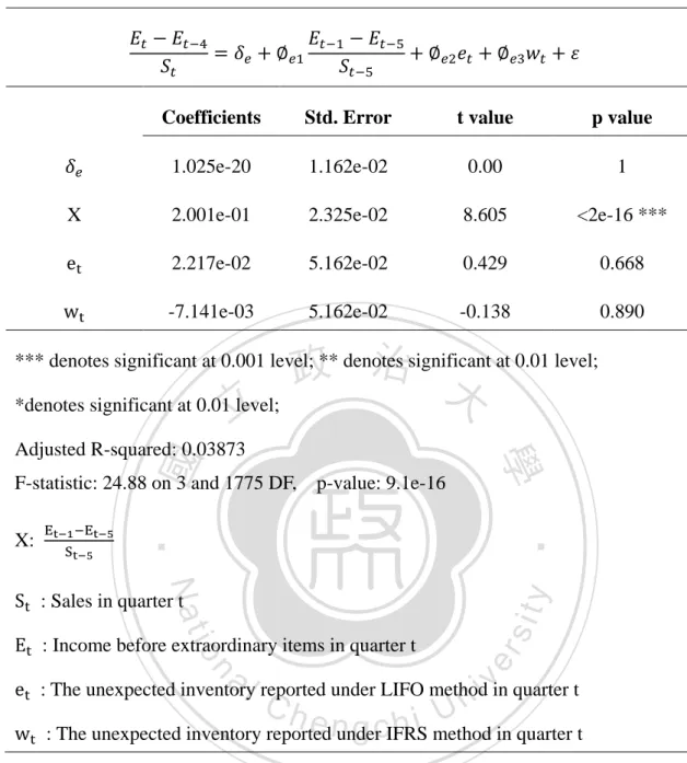
(33) According to Bernard (1991), when. is the inventory reported under LIFO. method, the residual. in the inventory expectations model is the proxy for LIFO. inventory, and when. is the inventory reported under IFRS method, the residual. in the inventory expectations model is the proxy for IFRS inventory. In the next section, the residual. and. will be added as regressor in the. sales, earnings and margin prediction equations. These regression models will be used to determine the inventories’ predictability of future sales and earnings. 3.4.3 Predicting Sales and Earnings with Inventory In this section, the residual. 立. 政治大 and from inventory expectations models are. added as regressor in the sales, earnings and margin prediction equations and develop. ‧ 國. 學. a new model. The purpose of the new models is to predict sales, earnings, and profit. ‧. margin with total inventory reported under LIFO and IFRS inventory valuation. sit. y. Nat. method, and determine which inventory valuation method can come up with inventory. io. al. er. levels which can be stronger indicators of future sales and earnings.. n. v i n C h and Profit Margins Final Sales, Earnings e n g c h i U Prediction Models. The prediction equations are as follows:. (7) (8) (9) : Sales in quarter t : Income before extraordinary items in quarter t : The unexpected inventory reported under LIFO method in quarter t : The unexpected total inventory reported under IFRS method in quarter t 26.

(34) If both. and. are positive, both IFRS and LIFO inventory are positively. related to future sales. The result is consistent with production smoothing model. If is significant and. is insignificant, IFRS inventory is the stronger indicator of. future sales, and hypothesis 1 is true. If. is significant and. is insignificant,. LIFO inventory is the stronger indicator of future sales, and hypothesis 1 is rejected. If both. and. are significant, and. is larger than. , IFRS inventory is. the stronger indicator of future sales and hypothesis 1 is true. If both are significant, and. is larger than. and. , LIFO inventory is the stronger indicator of. and 政治大 are 立negative, both IFRS and LIFO inventory are negatively. future sales and hypothesis 1 is rejected. The result is the same for If both. and. ‧ 國. significant and. is. 學. related to future sales. The result is consistent with stockout model. If. is insignificant, IFRS inventory is the stronger indicator of future. ‧. sales, and hypothesis 2 is true. If. is significant and. is insignificant, LIFO. y. sit. , IFRS inventory is the. v ni. n. al. is smaller than. er. are significant, and. io. and. Nat. inventory is the stronger indicator of future sales, and hypothesis 2 is rejected. If both. stronger indicator of future sales and hypothesis 2 is true. If both significant, and. Ch. is smaller than. and. are. e,nLIFO h i U is the stronger indicator of g cinventory. future sales and hypothesis 2 is rejected. The result is the same for. 27. and.

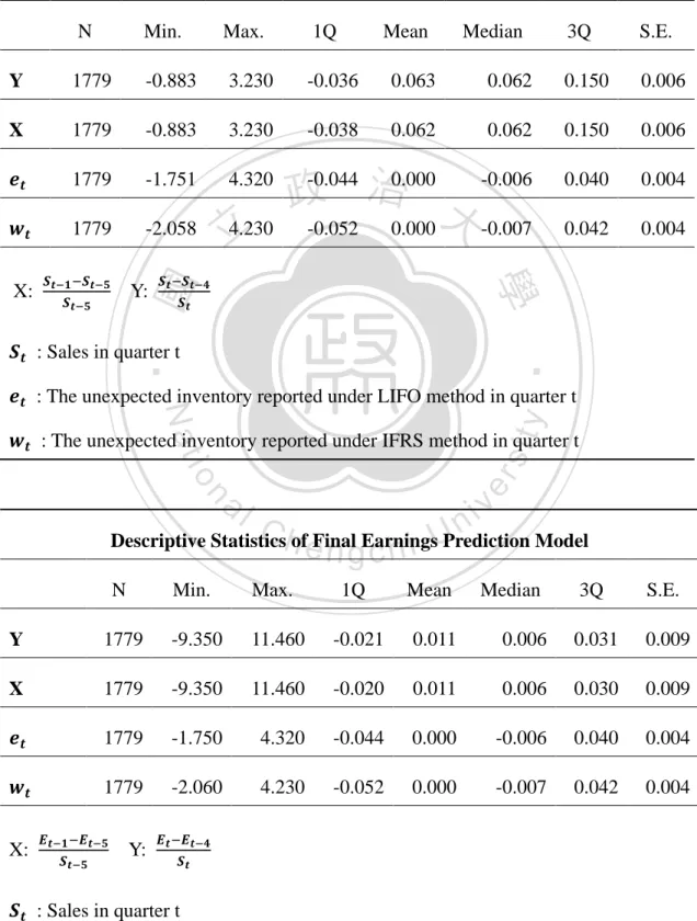
(35) 4. EMPIRICAL RESULTS AND ANALYSIS 4.1 Descriptive Statistic Table 4-1 Descriptive Statistics of Final Prediction Models Descriptive Statistics of Final Sales Prediction Model N. Min.. Max.. 1Q. Mean. Y. 1779. -0.883. 3.230. -0.036. 0.063. X. 1779. -0.883. 3.230. -0.038. 0.062. 1779. -1.751. 4.320. 1779. -2.058. 4.230 立. 3Q. S.E.. 0.062. 0.150. 0.006. 0.062. 0.150. 0.006. 0.040. 0.004. 0.042. 0.004. 政-0.044 治0.000 大 -0.006 -0.052. 0.000. -0.007. ‧ 國. 學. X:. Median. Y:. ‧. : Sales in quarter t. sit. y. Nat. : The unexpected inventory reported under LIFO method in quarter t. io. er. : The unexpected inventory reported under IFRS method in quarter t. al. n. v i n C Descriptive StatisticshofeFinal Earnings n g c h i UPrediction Model N. Min.. Max.. 1Q. Mean. Y. 1779. -9.350. 11.460. -0.021. 0.011. X. 1779. -9.350. 11.460. -0.020. 1779. -1.750. 4.320. 1779. -2.060. 4.230. X:. 3Q. S.E.. 0.006. 0.031. 0.009. 0.011. 0.006. 0.030. 0.009. -0.044. 0.000. -0.006. 0.040. 0.004. -0.052. 0.000. -0.007. 0.042. 0.004. Y: : Sales in quarter t 28. Median.

(36) : Income before extraordinary items in quarter t : The unexpected inventory reported under LIFO method in quarter t : The unexpected inventory reported under IFRS method in quarter t. Descriptive Statistics of Final Profit Margin Prediction Model N. Min.. Y. 1779. -1.350. 9.420. 0.018. 0.052. X1. 1779. -1.350. 9.420. 0.020. 0.052. X2. 1779. -4.090. 9.420. X3. 1779. -9.350. 政0.020 治0.050大 -0.021. 0.002. 3Q. S.E.. 0.050. 0.088. 0.006. 0.051. 0.088. 0.006. 0.052. 0.088. 0.006. 0.001. 0.023. 0.008. 0.040. 0.004. 0.042. 0.004. 4.320. -0.044. 0.000. -2.060. 4.230. -0.052. 0.000. -0.007. ‧ 國. -1.750. -0.006. io. y. al. n. : Sales in quarter t. sit. ; X3:. er. ; X2:. Median. Nat. X1:. Mean. ‧. 1779. 立9.390. 1Q. 學. 1779. Max.. Ch. : Income before extraordinary items in quarter t. engchi. i n U. v. : The unexpected inventory reported under LIFO method in quarter t : The unexpected inventory reported under IFRS method in quarter t The descriptive statistic results show that there is no extreme observation in the variables that reflects data distortion. The medians, means, first quartile and third quartile for independent variables and dependant variables are close, indicating that the distributions of the variables are quite normal.. 29.

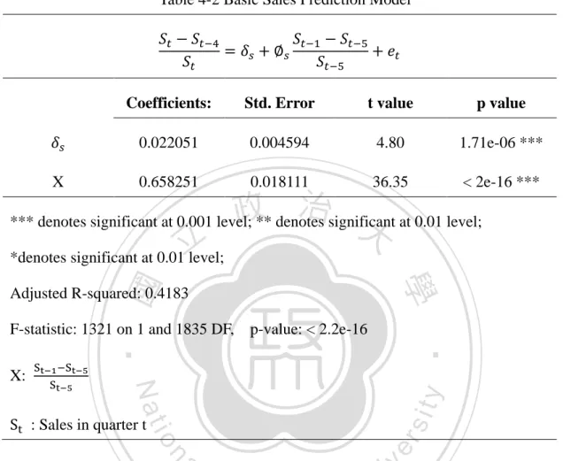
(37) 4.2 Empirical Results 4.2.1 Basic Prediction Model Table 4-2 Basic Sales Prediction Model. X. Coefficients:. Std. Error. t value. p value. 0.022051. 0.004594. 4.80. 1.71e-06 ***. 0.658251. 0.018111. 36.35. < 2e-16 ***. 政治大. *** denotes significant at 0.001 level; ** denotes significant at 0.01 level;. 立. *denotes significant at 0.01 level;. ‧ 國. 學. Adjusted R-squared: 0.4183 F-statistic: 1321 on 1 and 1835 DF,. ‧ sit. n. al. er. io. : Sales in quarter t. y. Nat. X:. p-value: < 2.2e-16. i n U. v. Table 4-2 reports the estimates of the Basic Sales Prediction Model. X is equal to. Ch. engchi. the first lag seasonal difference in sales scaled by the base quarter. The model shows that the first lag seasonal difference in sales explains much of the current seasonal difference in sales, with the R-squared equals 0.4183. The coefficient on the first lag seasonal difference in sales is positive and significant at 0.001 level, indicating that the variable is positively and highly related to current seasonal difference in sales, and the variable is a necessary control variable in forming sales prediction.. 30.

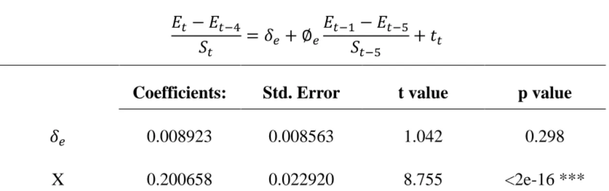
(38) Table 4-3 Basic Earnings Prediction Model. X. Coefficients:. Std. Error. t value. p value. 0.008923. 0.008563. 1.042. 0.298. 0.200658. 0.022920. 8.755. <2e-16 ***. *** denotes significant at 0.001 level; ** denotes significant at 0.01 level; *denotes significant at 0.01 level; Adjusted R-squared: 0.03957. 立. 政治大. F-statistic: 76.65 on 1 and 1835 DF,. ‧ 國. 學. X:. p-value: < 2.2e-16. ‧. : Sales in quarter t. sit. y. Nat. : Income before extraordinary items in quarter t. n. al. er. io. Table 4-3 reports the estimates of the Basic Earnings Prediction Model. X is. v. equal to the first lag seasonal difference in earnings scaled by the base quarter. The. Ch. engchi. i n U. R-squared is equal to 0.03957. This shows that the first lag seasonal difference in earnings doesn’t explain the current seasonal difference in earnings well. However, the coefficient on the first lag seasonal difference in earnings is positive and significant at 0.001 level, implying that there is still a strong association between the first lag seasonal difference in earnings and current seasonal difference in earnings, and the variable is a necessary control variable in forming earnings prediction.. 31.

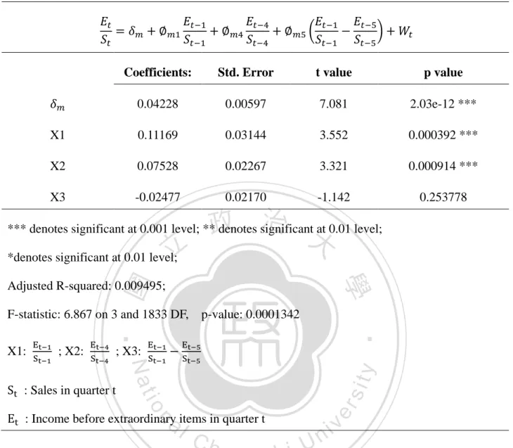
(39) Table 4-4 Basic Profit Margins Prediction Model. Coefficients:. Std. Error. t value. p value. 0.04228. 0.00597. 7.081. 2.03e-12 ***. X1. 0.11169. 0.03144. 3.552. 0.000392 ***. X2. 0.07528. 0.02267. 3.321. 0.000914 ***. X3. -0.02477. 0.02170. -1.142. 0.253778. 政治大. *** denotes significant at 0.001 level; ** denotes significant at 0.01 level;. 立. *denotes significant at 0.01 level;. ‧ 國. 學. Adjusted R-squared: 0.009495; F-statistic: 6.867 on 3 and 1833 DF, ; X3:. io. sit. y. Nat. : Sales in quarter t. al. n. : Income before extraordinary items in quarter t. Ch. engchi. er. ; X2:. ‧. X1:. p-value: 0.0001342. i n U. v. Table 4-4 reports the estimates of the Basic Profit Margins Prediction Model. X1 is the first lag profit margins, X2 is the fourth lag profit margins, and X3 is the first lag seasonal difference in profit margins. The R-squared is equal to 0.009495. This shows that the Independent variables in profit margins cannot explain much of the current profit margins. However, the coefficients on all the independent variables are positive and significant at 0.001 levels, indicating that there is still a strong association between these variables and current profit margins. The estimates of are significant, suggesting that the model used for sales and earnings would have been inadequate for profit margins. The estimates of 32. are significant, suggesting the.

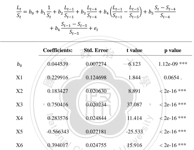
(40) presence of seasonality in margins. The estimates of. are not significant,. conforming the stationarity in the series. 4.2.2 Inventory Expectations Models Table 4-5 Inventory Expectations Model—LIFO method. Coefficients:. 立. 1.12e-09 ***. 0.124698. 1.844. 0.0654 .. 0.183427. 0.020630. 8.891. < 2e-16 ***. 0.750416. 0.020234. 37.087. ‧. < 2e-16 ***. 0.283576. 0.024844. 11.414. < 2e-16 ***. X5. -0.566343. 0.022181. -25.533. X6. 0.394017. Nat. X4. io. n. al. sit. X3. er. X2. ‧ 國. 0.229916. 學. X1. p value. y. 0.044539. Std. Error 治 t value 政大6.123 0.007274. Ch. 0.024755. engchi. i n U. v. 15.916. < 2e-16 *** < 2e-16 ***. *** denotes significant at 0.001 level; ** denotes significant at 0.01 level; *denotes significant at 0.01 level Adjusted R-squared: 0.8049 F-statistic: 1264 on 6 and 1830 DF, p-value: < 2.2e-16 X1:. ; X2:. ; X3:. ; X4:. ; X5:. ; X6:. : Sales in quarter t : Total inventory under LIFO method in quarter t Table 4-5 reports the estimates of the LIFO Inventory Expectations Model. The 33.

(41) model explains much of the variance in inventories, with the R-squared equals 0.8049. The coefficients on the fourth lag of inventory-to-sales ratio and the first lag in seasonal difference are both positive and significant at 0.001 levels, indicating that these variables are necessary control variables in forming inventory expectations. The coefficients in the LIFO inventory expectations model show that the LIFO inventory-to-sales ratios are negatively and significantly related to current sales, indicating that production cannot adjust instantaneously to demand changes, and that inventory-to-sales ratios decline as sales increase. According to Bernard (1991), if. 政治大 current inventory-to-sales and 立past sales, as production is adjusted for inventory. inventory is a buffer for sales, there should also be a positive relationship between. ‧ 國. 學. excesses or shortfalls in the previous quarter. This is the case, with current inventory-to-sales ratios positively related to sales changes lagged on quarter, and the. ‧. coefficient roughly equal in magnitude to the coefficient on current sales changes. The. sit. y. Nat. buffering behavior is consistent with the stockout model of inventory, while it is. n. al. er. io. inconsistent with production smoothing model, for which inventory-to-sales ratios would be a leading indicator of sales.. Ch. engchi. 34. i n U. v.

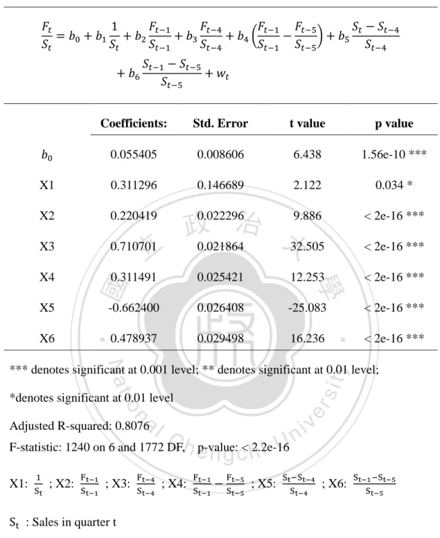
(42) Table 4-6 Inventory Expectations Models—IFRS method. Coefficients:. Std. Error. t value. p value. 0.055405. 0.008606. 6.438. 1.56e-10 ***. X1. 0.311296. 0.146689. 2.122. 0.034 *. X2. 0.220419. X3. 0.710701. X4. 0.311491. 0.025421. 12.253. < 2e-16 ***. -0.662400. 0.026408. -25.083. < 2e-16 ***. 0.478937. 0.029498. 16.236. ‧ 國. < 2e-16 ***. ‧. X6. < 2e-16 ***. 學. X5. 立. 0.022296 9.886 政治大 0.021864 32.505. < 2e-16 ***. Nat. sit. y. *** denotes significant at 0.001 level; ** denotes significant at 0.01 level;. er. io. *denotes significant at 0.01 level. n. al. i n C F-statistic: 1240 on 6 and 1772 DF,h e p-value: < 2.2e-16 ngchi U Adjusted R-squared: 0.8076. X1:. ; X2:. ; X3:. ; X4:. ; X5:. v. ; X6:. : Sales in quarter t : Total inventory under IFRS method in quarter t Table 4-6 reports the estimates of the IFRS Inventory Expectations Model. The model explains the variance in inventories well, with the R-squared equals 0.8076. The coefficient on the fourth lag of inventory-to-sales ratio and the first lag in seasonal difference are both positive and significant at 0.001 levels, indicating that 35.

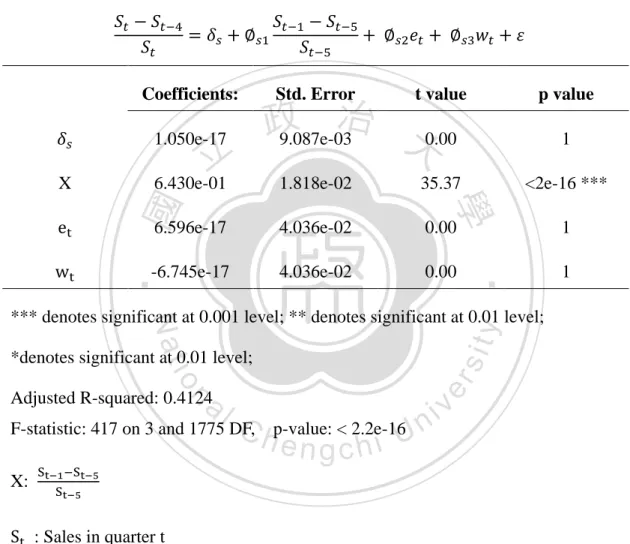
(43) these variables are essential control variables in forming inventory expectations. The IFRS inventory are also negatively related to current sales changes and positively related to first lag sales changes, indicating the buffer effect of first lag sales change.. 4.3 Final Prediction Models Table 4-7 Final Sales Prediction Model. Coefficients: 1.050e-17. 立. 6.430e-01. t value. p value. 治政 9.087e-03 大0.00. 1. 35.37. <2e-16 ***. 6.596e-17. 4.036e-02. 0.00. 1. -6.745e-17. 4.036e-02. 0.00. 1. 學. 1.818e-02. ‧. ‧ 國. X. Std. Error. sit. y. Nat. *** denotes significant at 0.001 level; ** denotes significant at 0.01 level;. io. er. *denotes significant at 0.01 level;. al. n. Adjusted R-squared: 0.4124. F-statistic: 417 on 3 and 1775 DF, C hp-value: < 2.2e-16U n i engchi. v. X: : Sales in quarter t : The unexpected inventory reported under LIFO method in quarter t : The unexpected inventory reported under IFRS method in quarter t In the final prediction models, the residuals from the inventory expectations model are added as a regressor in prediction models for sales, earnings, and margins to evaluate the predictive ability of inventory. Table 4-7 reports the estimates of the Final Sales Prediction Model. The model shows that the first lag seasonal difference 36.

(44) in sales explains the current seasonal difference in sales quite well, with the R-squared equals 0.4183. The coefficient on the first lag seasonal difference in sales is positive and significant at 0.001 level, indicating that the variable is strongly related to current seasonal difference in sales. In the model,. is the estimated unexpected inventory from LIFO inventory. expectations model, and. is the estimated unexpected inventory from IFRS. inventory expectations model. According to Bernard and Stober (1989), if the production smoothing model holds, the unexpected inventory would contain. 政治大 sales and earnings increases. 立If the stockout model holds, then unexpected inventory information about future demand, and positive unexpected inventory would predict. ‧ 國. 學. would contain information about the difference between current sales and current demand, and positive unexpected inventory would predict sales and earnings decrease.. ‧. If neither of these models hold and the simple decision rules are adequate to describe. sit. y. Nat. the production decision, then unexpected inventory is noise, and would not be able to. n. al. and. represent. er. io. predict future sales or earnings. As a result, the coefficients of. i n U. v. either the ability of LIFO inventory and IFRS inventory to predict future sales, or the noises in the models.. Ch. engchi. Table 4-7 shows the positive relation between unexpected inventory and future sales for LIFO inventory, and negative relation between the two variables for IFRS inventory. The results show that the predictability of LIFO inventory for future sales tends to be consistent with production smoothing model, while the predictability of IFRS inventory for future sales tend to be consistent with stockout model. However, the coefficients on both LIFO and IFRS inventory are statistically insignificant. These results indicate that the effect of production smoothing model and stockout model on inventory is not significant. 37.

(45) Table 4-8 Final Earnings Prediction Model. X. Coefficients. Std. Error. t value. p value. 1.025e-20. 1.162e-02. 0.00. 1. 2.001e-01. 2.325e-02. 8.605. <2e-16 ***. 2.217e-02. 5.162e-02. 0.429. 0.668. -7.141e-03. 5.162e-02. -0.138. 0.890. 政治大. *** denotes significant at 0.001 level; ** denotes significant at 0.01 level;. 立. *denotes significant at 0.01 level;. ‧ 國. F-statistic: 24.88 on 3 and 1775 DF,. p-value: 9.1e-16. ‧. X:. 學. Adjusted R-squared: 0.03873. y. Nat. n. al. er. io. : Income before extraordinary items in quarter t. sit. : Sales in quarter t. i n U. v. : The unexpected inventory reported under LIFO method in quarter t. Ch. engchi. : The unexpected inventory reported under IFRS method in quarter t Table 4-8 reports the estimates of the Final Earnings Prediction Model. The model shows that the independent variables do not explain the dependent variable well, with the R-squared equals 0.03873. The coefficient on the first lag seasonal difference in earnings is positive and significant at 0.001 level, indicating that there is a strong association between the two variables. The results show a positive relation between unexpected inventory and future earnings for LIFO inventory, and a negative relation for the two variables for IFRS 38.

(46) inventory, implying the smoothing effect for LIFO inventory and stockout effect for IFRS inventory. However, the coefficients on both LIFO and IFRS inventory are statistically insignificant, indicating that neither production smoothing nor stockout model holds. The unexpected inventories from LIFO inventory and IFRS inventory may be the noises in the models. Table 4-9 Final Profit Margins Prediction Model. Std. Error t value 治政大 0.000 1.181e-02. Coefficients. 立. 1.076e-01. 0.000768***. 7.893e-02. 2.482e-02. 3.180. 0.001498 **. -3.356e-02. 3.142e-02. -1.068. 3.752e-02. 5.246e-02. 0.715. -3.960e-02. 5.244e-02. -0.755. n. Ch. 0.474607. sit. io. al. 0.285711. er. X3. y. 3.370. ‧ 國. 3.192e-02. ‧. 1.076e-01. 學. X2. i n U. v. *** denotes significant at 0.001 level; ** denotes significant at 0.01 level; *denotes significant at 0.01 level;. engchi. Adjusted R-squared: 0.03873 F-statistic: 3.876 on 5 and 1773 DF, X1:. ; X2:. 1.000000. Nat. X1. p value. p-value: 0.001695. ; X3:. : Sales in quarter t : Income before extraordinary items in quarter t : The proxy of total inventory reported under LIFO method in quarter t : The proxy of total inventory reported under IFRS method in quarter t 39. 0.450262.

(47) Table 4-9 reports the estimates of the Final Profit Margins Prediction Model. The R-squared is equal to 0.03873, suggesting that the independent variables do not explain the dependent variable well. The coefficient on the first lag seasonal difference in profit margins is positive and significant at 0.001 level, indicating a strong relation between the dependent and independent variables. The results once again show that the unexpected inventory is a positive leading indicator of profit margins for LIFO inventory, but a negative leading indicator of profit margins for IFRS inventory. The coefficients for LIFO and IFRS inventory are. 政治大 effect are not prevailed. The 立unexpected inventories from LIFO inventory and IFRS statistically insignificant suggest that the production smoothing effect and stockout. ‧. ‧ 國. 學. inventory are the noises in the models.. n. er. io. sit. y. Nat. al. Ch. engchi. 40. i n U. v.

(48) 5. Conclusion In economic literature, production smoothing model and stockout model address the predictability of inventory disclosure on sales and earnings. Based on these models, Bernard and Noel (1991) show that inventory disclosure predicts sales and earnings. This study further investigates and compares the predictability of the sales and earnings by inventory reported under last in, last out (LIFO) and that under International Accounting Standard 2 (IAS 2). Thus this study compares the predicting ability of inventory on sales and earnings under IFRS and non-IFRS.. 政治大 This study selects a group of companies adopting LIFO and disclosing LIFO 立. reserves to be the sample companies, and the LIFO reserves are added to the. ‧ 國. 學. inventories reported under LIFO method to generate the inventories reported under. ‧. IFRS inventory valuation method. IFRS inventory valuation method is defined as the. sit. y. Nat. inventory valuation methods recommended under IAS 2, which may be FIFO method. io. er. or weighted average method and can reflect a company’s internal inventory policy. The sales, earnings, and profit margins models developed by Bernard are used to. al. n. v i n C h and IFRS inventory determine the ability of LIFO inventory to predict sales, earnings, engchi U and profit margins, and whether LIFO inventory has better predictability than IFRS inventory. The empirical results show a positive relation between the LIFO unexpected inventory and current sales and earnings, and a negative relation between IFRS unexpected inventory and current sales and earnings. However, the coefficients for the unexpected inventories under LIFO and IFRS are both statistically insignificant, suggesting that the unexpected inventories are merely noises in the models, and that the effects of production smoothing model and stockout model are not prevailed and 41.

(49) may be inadequate to explain the management’s inventory policies and decisions. Thus, it is difficult to determine which inventory valuation method can generate the inventory that leads to better sales and earnings prediction.. 立. 政治大. ‧. ‧ 國. 學. n. er. io. sit. y. Nat. al. Ch. engchi. 42. i n U. v.

(50) REFERENCES Abarbanell, J., and B. Bushee. 1997. ―Fundamental analysis, future earnings and stock prices.‖ Journal of Accounting Research 35 (1): 1–24. Aror, Shveta. 2011. ―Grocery Retail: The Next Level of Inventory Management.‖ Retail Merchandiser 51(3): 26-28. Bar-Yosef, S, and P. K. Sen. 1992. "On Optimal Choice of Inventory Accounting Method.'' The Accounting Review (April): 320-36.. 政治大 Journal of Accounting,立 Auditing and Finance (Spring):145-181.. Bernard, V. and Noel, J. 1991 ―Do Inventory Disclosures Predict Sales and Earnings?‖. ‧ 國. 學. Bernard, V., and T. Stober. 1989. The nature and amount of information reflected in cash flows and accruals. The Accounting Review 64 (October): 624-652.. ‧. sit. y. Nat. Blinder, A. 1986 ―Can the Production Smoothing Model of Inventory Be Saved?‖ The. io. al. er. Quarterly Journal of Economics (August): 431-453.. v. n. Biddle, G. C., and Ricks, W. E. 1988. ―Analyst forecast errors and stock price. Ch. engchi. i n U. behavior near the earnings announcement dates of LIFO adopters.‖ Journal of Accounting Research, 26(2):169-194. Brown, Jeff. 2008/2009. ―Consumer Driven Forecasting To Improve Inventory Flow: Brown Shoe Company’s Journey.‖ Journal of Business Forecasting 27 (Winter): 24-25. Cushing, B. E., and LeClere, M. J. 1992. ―Evidence on the determinants of inventory accounting policy choice.‖ The Accounting Review 67(2): 355–366. Chi-Wen Jevons Lee. 1988. ―Inventory accounting and earnings/price ratios: A puzzle‖ 43.

(51) Contemporary Accounting Research 5 (Fall): 371-388. Foster, G. 1977 ―Quarterly Accounting Data: Time-Series Properties and Predictive-Ability Results.‖ The Accounting Review (January): 1-21. Guenther, D. A., & Trombley, M. A. 1994. ―The ’LIFO reserve’ and the value of the firm: Theory and empirical evidence.‖ Contemporary Accounting Research 10(2): 433–452. Gupta, Mahendra, Pevzner, Mikhail; Seethamraju, Chandra. 2010. ―The Implications. 政治大 Performance and Valuation.‖ Contemporary Accounting Research 27 (Fall): 立 of Absorption Cost Accounting and Production Decisions for Future Firm. 889-922.. ‧ 國. 學. Guido Lorenzoni 2006. ―A Theory of Demand Shocks.‖ MIT Economics.. ‧. Hand, J. 1993. ―Resolving LIFO Uncertainty; A Theoretical and Empirical. y. Nat. al. er. io. Accounting Research 31 (Spring): 21-49.. sit. Reexamination of 1974-75 LIFO Adoption and Nonadoptions.‖ Journal of. n. v i n Ch Hughes, P. J., Schwartz, E. S., Fellingham, J. & Thakor, A. V. 1994. ―Continuous engchi U. signaling within partitions: Capital structure and the FIFO/LIFO choice.‖ Journal of Accounting, Auditing & Finance 9(1): 1–19.. International Accounting Standard 2 ―Inventories.‖ International Accounting Standards Board. Jennings, R., Mest, D. P., and Thompson, R. B. II. 1992. ―Investor reaction to disclosures on 1974–75 LIFO adoption decisions.‖ The Accounting Review 67(2): 337–354. Jennings, R., Simko, J. P. and Thompson, R.B. II. 1996. ―Does LIFO Inventory 44.

(52) Accounting Improve the Income Statement at the Expense of the Balance Sheet?‖ Journal of Accounting Research, 34(1) (Spring): 85-109. Kang, S.-H. 1993. ―A conceptual framework for the stock price effects of LIFO tax benefits.‖ Journal of Accounting Research 31(1): 50–61. Kahn, J. 1987. ―Inventories and the Volatility of Production.‖ The American Economic Review (September): 667-679. Lev, B., and R. Thiagarajan. 1993. ―Fundamental information analysis.‖ Journal of. 政治大 Thomas, J., and H. Zhang. 立 2003. ―Inventory changes and future returns.‖ Review of Accounting Research 31 (3): 190–215.. ‧. ‧ 國. 學. Accounting Studies 7 (2–3): 163–87.. n. er. io. sit. y. Nat. al. Ch. engchi. 45. i n U. v.

(53)