微型陀螺儀的強健控制器設計

全文

(1)國立. 交通大學. 電機與控制工程研究所碩士論文. 微型陀螺儀的強健控制器設計 Design of Robust Controller for Micro Vibratory Ring Gyroscope. 研究生：楊昇儒指導教授：邱一博士. 中華民國九十七年十月.

(2) 微型陀螺儀的強健控制器設計 Design of Robust Controller for Micro Vibratory Ring Gyroscope. 研究生: 楊昇儒. Student: S. R. Yang. 指導教授: 邱一. Advisor: Yi Chiu 國立交通大學電機學院電機與控制工程研究所碩士論文. A Thesis Submitted to Department of Electrical and Control Engineering College of Electrical Engineering National Chiao Tung University In Partial Fulfillment of the Requirement For the Degree of Master In Electrical and Control Engineering October 2008 Hsinchu, Taiwan, R.O. C 中華民國九十七年十月.

(3) 中文摘要. 隨著微機電科技的進步，微型陀螺儀的應用日益廣泛，如在汽車的導航及安全控制、遊戲主機、手機等都可發現其蹤跡。對於目前的微機電式陀螺儀而言，製造過程中的誤差及使用過程中的磨損會造成成品與設計間存在差異，以至於無法滿足原先系統的規格。本研究的重點在於設計一控制器，能在微型陀螺儀的特性參數發生變異時，還能保有一定的系統性能。因為陀螺儀本身屬於多輸入多輸出系統 (multi-input multi-output, MIMO)，且驅動軸與感測軸間有耦合的情形，若系統特性有變異時，無法利用一般的 PID 控制設計方法來達成規格要求。因此，我們必須設計一個既可以控制 MIMO 系統又可以忍受特性參數變異的穩健控制器(robust controller)。在此論文中我們會先忽略系統變異並利用 pole placement 的控制理論設計出 PID 控制器，之後再利用穩健控制理論中的 H∞理論結合量化迴授理論(quantitative feedback theory, QFT) 設計出穩健控制器，最後比較不同控制器的性能和穩健特性等差異。論文中，我們先找出受控體的特性矩陣 P(s)和權重函數，並使用 MATLAB 輔助完成控制器的設計。當系統的共振頻率和阻尼係數存在 10%變異量時，加入 PID 控制的系統響應變異量為 24%，而加入 QFT/H∞控制器的變異量為 5.6%，且暫態響應的特性仍能符合規格，包含安定時間小於 0.2ms，最大超越量低於 10%，可知利用 QFT/H∞的控制方法設計出的控制器在穩健性上有明顯的改善。此外和一般 H∞控制器相比，系統迴路由狀態回授變為輸出回授，因而在實現上也較為容易。. i.

(4) Abstract With the progress of the MEMS technology, the application of micro-gyroscopes becomes more and more extensive. Examples can be found in automobile navigation and safety control, game hosts, mobile phones, etc.. However, fabrication errors and operation wearout will cause difference in component characteristics between the expected value and the actual value in real devices. The objective of this research is focused on the design of a controller which can maintain certain system performance in the presence of the system characteristic parameter variation. The gyroscope is a multi-input multi-output (MIMO) system with possible variations in system characteristics. Therefore, the common PID controller design method can not be used in controller design to meet the specification. A robust controller which can be used to control a MIMO system and endure parameter variation is required. In this thesis, the pole placement method is applied to design a PID controller without considering the system variation. Then the H∞ theory and quantitative feedback theory (QFT) are applied to design the controller. The performance and the robustness of the controllers are compared. After determining the characteristic matrix P of the plant and the weighting functions, the controller is calculated by MATLAB. When the natural frequency and the damping coefficient both have variation of 10%, the variation of the system response is 5.6% in QFT/H∞ controller and 24% in PID controller. Therefore, the QFT/H∞ control method has better robustness. Compared with conventional H∞ controller, the QFT/H∞ control loop uses output feedback and is easier to realize.. ii.

(5) 致謝兩年的碩士班生涯即將結束，這段時間對我而言是人生中不可缺乏的階段，我感到獲益良多。首先要謝謝我的指導教授邱一老師，他總是給我許多專業的意見和方向，也教導了我正確的學習態度以及研究精神，且不厭其煩的給我指導，使我在他身上學到許多，在此要真心的感謝老師，「老師！您辛苦了！」此外要謝謝我的口試委員，邱俊誠博士和蕭得聖博士，謝謝您們給我的種種意見，讓我發現許多考慮不周詳的地方。兩年的時間，有辛苦也有歡樂，這都要感謝實驗室的成員們。感謝實驗室的學長：忠衛、炯廷、建勳、均宏、亦謙、繁果和煒智，謝謝你們這段時間來傳授我許多實驗上的經驗和知識；感謝陪伴我兩年和我一起努力的同學：子麟、弘諳、昌修，這段時間咱們互相勉勵互相扶持，我不會忘記你們的，期望以後畢業後仍有相聚的機會；感謝帶給我歡樂的學弟妹：建安、經富、鴻智、政安、俊宏、姿穎、哲明，在接近畢業的時候，許多雜事都落到了你們身上，辛苦你們了。接著要感謝我的父母和家人，因為有你們幫忙，讓我不愁吃穿，且在我遇到困難和失落時，給我支持和鼓勵。特別要感謝的是我的女友慧萱，感謝妳這段時間給我的鼓勵和幫助，妳是讓我支持下去的最重要因素，謝謝妳！最後，謝謝曾經幫助過我的人，畢業之後就要離開校園踏入職場，期許自己能將這兩年的所學經驗，充分運用在之後的日子，為社會盡我微薄之力。. 楊昇儒謹識中華民國九十七年十月新竹交大. iii.

(6) Table of Content 中文摘要......................................................................................................................... i Abstract .........................................................................................................................ii 致謝.............................................................................................................................. iii Table of Content .......................................................................................................... iv List of Figures .............................................................................................................. vi List of Tables................................................................................................................ ix Chapter 1 Introduction .......................................................................................... 1 1.1 Gyroscope ...................................................................................................... 2 1.1.1 MEMS gyroscope .......................................................................... 2 1.1.2 Vibrating beam gyroscope ............................................................. 3 1.1.3 Tuning fork gyroscope ................................................................... 4 1.1.4 Vibrating ring gyroscope................................................................ 5 1.1.5 Frame gyroscope ............................................................................ 5 1.2 Gyroscope control .......................................................................................... 6 1.2.1 Adaptive control............................................................................. 6 1.2.2 H∞ control ..................................................................................... 7 1.2.3 AGC force rebalance control ......................................................... 8 1.2.4 Active disturbance rejection control .............................................. 9 1.2.5 Summary ...................................................................................... 10 1.3 Objectives and thesis organization ............................................................... 11 Chapter 2 Principle of MEMS gyroscope .......................................................... 12 2.1 Operating principle ...................................................................................... 13 2.1.1 Non-ideal effects .......................................................................... 15 2.1.2 Open-loop mode of operation ...................................................... 16 2.1.3 Closed-loop mode of operation .................................................... 17 2.2 Equation of motion....................................................................................... 17 2.2.1 Ideal plant..................................................................................... 17 2.2.2 Non-ideal plant............................................................................. 18 2.3 Parameters of the MEMS gyroscope ........................................................... 19 2.4 Force balance control ................................................................................... 22 2.5 Demodulation ............................................................................................... 23 2.6 Summary ...................................................................................................... 24 Chapter 3 Controller design ................................................................................ 26 3.1 System analysis ............................................................................................ 26 3.1.1 Characteristics in time domain..................................................... 26 iv.

(7) 3.1.2 Characteristics in frequency domain ............................................ 27 3.2 PID control design using pole placement .................................................... 28 3.2.1 PID controller............................................................................... 29 3.2.2 Pole placement method ................................................................ 29 3.2.3 Using pole placement to design PID controller ........................... 30 3.3 QFT/H∞ Control .......................................................................................... 31 3.3.1 3.3.2 3.3.3 3.3.4 3.3.5. QFT design technique .................................................................. 32 H∞ control method [22] ............................................................... 33 Combined QFT/H∞ control .......................................................... 35 Design of QFT/H∞ controller for MEMS gyroscope................... 38 QFT/H∞ method discussion ........................................................ 40. 3.4 Summary ...................................................................................................... 40 Chapter 4 Simulation and Discussion ................................................................ 42 4.1 Open-loop system ........................................................................................ 42 4.1.1 Model verification ........................................................................ 43 4.1.2 Simulation .................................................................................... 45 4.2 PID controller using pole placement ............................................................ 49 4.3 QFT/H∞ control ........................................................................................... 52 4.4 Robustness ................................................................................................... 57 4.5 Comparison with other publications ............................................................ 60 4.5.1 4.5.2. AGC force rebalance control ....................................................... 60 H∞ control ................................................................................... 61. 4.6 Summary ...................................................................................................... 63 Chapter 5 Conclusion and Future Work............................................................ 64 5.1 Conclusion ................................................................................................... 64 5.2 Future work .................................................................................................. 64 References ................................................................................................................... 66. v.

(8) List of Figures Fig. 1.1 A prototype bulk-micromachined gyroscope, diced and released [6] .............. 3 Fig. 1.2 Vibrating beam gyroscope [10] ........................................................................ 4 Fig. 1.3 Tuning fork MEMS gyroscope [11] ................................................................. 4 Fig. 1.4 Vibrating ring gyroscope [12]........................................................................... 5 Fig. 1.5 Frame gyroscope [13] ....................................................................................... 6 Fig. 1.6 Block diagram of the adaptive add-on control [14] .......................................... 7 Fig. 1.7 (a) Plant model, (b) block diagram of MEMS gyroscope with H∞ controller [4] ....................................................................................................................... 8 Fig. 1.8 (a) Force rebalance configuration with a modified AGC loop, (b) block diagram and electronics for force rebalance [16] .............................................. 9 Fig. 1.9 Block diagram of the ADRC and rate estimation [5] ..................................... 10 Fig. 2.1 Overview of the micro vibrating ring gyroscope............................................ 12 Fig. 2.2 Concept of the Coriolis acceleration .............................................................. 13 Fig. 2.3 Resonant modes of a vibrating ring gyroscope (a) drive mode, (b) sense mode .......................................................................................................................... 14 Fig. 2.4 Response of the overall 2-DOF system with varying drive and sense stiffness mismatch [6]. ................................................................................................... 16 Fig. 2.5 layout of the micro vibrating ring gyroscope ................................................. 20 Fig. 2.6 Modal analysis (a) mode1, (b) mode2, (c) mode3, (d) mode4 ....................... 21 Fig. 2.7 Control loop of two axes ................................................................................ 23 Fig. 3.1 Step response of MEMS gyroscope................................................................ 27 Fig. 3.2 Bode plot of MEMS gyroscope plant ............................................................. 28 Fig. 3.3 Schematic of the closed-loop system with a PID controller ........................... 29 Fig. 3.4 Schematic of the general closed-loop system with QFT/H∞ controller......... 31 Fig. 3.5 Unity feedback closed-loop for different plant cases [17].............................. 33 Fig. 3.6 H∞ control structure ........................................................................................ 34 Fig. 3.7 QFT/H∞ design step ....................................................................................... 36 Fig. 3.8 Multiplicative perturbation model of the plant ............................................... 37 Fig. 3.9 Flow chart of combined QFT/H∞ design ....................................................... 39 Fig. 3.10 Frequency response of the closed-loop system, x(s)/r(s), with controller designed by QFT/H∞ method .......................................................................... 40 Fig. 4.1 Simulink model of the gyroscope (a) overview (b) detail of Subsystem for drive axis (c) detail of Subsystem for sense axis ............................................. 42 Fig. 4.2 Harmonic analysis .......................................................................................... 44 Fig. 4.3 Deformation of the structure at resonance ...................................................... 44 vi.

(9) Fig. 4.4 Harmonic response of the finite element model ............................................. 45 Fig. 4.5 Simulink model of the open-loop system ....................................................... 46 Fig. 4.6 Input force on the drive axis in the open-loop system .................................... 46 Fig. 4.7 Coriolis force from the drive axis on the sense axis in the open-loop system 46 Fig. 4.8 Displacement of the drive axis in the open-loop system ................................ 47 Fig. 4.9 Displacement of the sense axis in the open-loop system................................ 47 Fig. 4.10 Force on the sense axis in the open-loop system with quadrature error ....... 48 Fig. 4.11 Displacement of the sense axis in the open-loop system with quadrature error .................................................................................................................. 48 Fig. 4.12 Simulink model of the closed-loop system with a PID controller ................ 49 Fig. 4.13 Controller output on the drive axis in the closed-loop system with a PID controller .......................................................................................................... 50 Fig. 4.14 Controller output on the sense axis in the closed-loop system with a PID controller .......................................................................................................... 51 Fig. 4.15 Displacement of the drive axis in the closed-loop system with a PID controller .......................................................................................................... 51 Fig. 4.16 Displacement of the sense axis in the closed-loop system with a PID controller .......................................................................................................... 51 Fig. 4.17 Effect of the PID controller on the displacement of the sense axis .............. 52 Fig. 4.18 Angular rate of the close-loop system with a PID controller ....................... 52 Fig. 4.19 Simulink model of the closed-loop system with a QFT/H∞ controller........ 53 Fig. 4.20 Controller output on the drive axis in the closed-loop system with a QFT/H∞ controller .......................................................................................................... 54 Fig. 4.21 Controller output on the sense axis in the closed-loop system with a QFT/H∞ controller .......................................................................................................... 55 Fig. 4.22 Displacement of the drive axis in the closed-loop system with a QFT/H∞ controller .......................................................................................................... 55 Fig. 4.23 Displacement of the sense axis in the closed-loop system with a QFT/H∞ controller .......................................................................................................... 55 Fig. 4.24 Angular rate of the close-loop system with a QFT/H∞ controller ............... 56 Fig. 4.25 Feedback force of sense axis of close-loop system by QFT/H∞ control with and without prefilter ......................................................................................... 56 Fig. 4.26 Angular rate of close-loop system by QFT/H∞ control with and without prefilter ............................................................................................................. 56 Fig. 4.27 Robustness comparisons of three controllers (a) without system variation, (b) with 10% variation in natural frequency, (c) with 10% variation in damping coefficient, (d) with 10% variation in both the natural frequency and damping coefficient ........................................................................................................ 59 vii.

(10) Fig. 4.28 Simulation result with QFT/H∞ control ....................................................... 61 Fig. 4.29 Step response of the simulation results [16] ................................................. 61 Fig. 4.30 Controller output resonant frequency variation by H∞ controller in [4]...... 62 Fig. 4.31 Simulation result with QFT/H∞ control ....................................................... 62. viii.

(11) List of Tables Table 2.1 System parameters ....................................................................................... 22 Table 2.2 System specifications ................................................................................... 22 Table 3.1 Characteristics in time and frequency domains ........................................... 28 Table 3.2 PID controller gain ....................................................................................... 31 Table 4.1 Calculated and simulated response amplitude of the open-loop system ...... 49 Table 4.2 Simulation results of the closed-loop system with a PID controller for Ω= 100°/sec ............................................................................................................ 52 Table 4.3 Simulation results of the closed-loop system with a QFT/H∞ controller for Ω = 100°/sec .................................................................................................... 57 Table 4.4 Robustness comparison ................................................................................ 59 Table 4.5 Robustness comparison with frequency mismatch ...................................... 60 Table 4.6 Dynamic parameters of that MEMS vibratory gyroscope in [16]................ 60. ix.

(12) Chapter 1. Introduction. Gyroscopes are used to measure the angular rate in vehicle navigation, guidance, rollover stability, and in aerospace applications such as aircrafts and satellites. Therefore, the accuracy and precision of gyroscopes have been the targets of intensive studies. Gyroscopes have been developed for a long time, but traditional gyroscopes are too big and expensive. Therefore, MEMS gyroscopes are becoming more popular in electronic and consumer market. Micro Electro-Mechanical Systems (MEMS) have the advantages of small dimensions, mass production, and integration with electronic circuits. It has been used in various sensing applications, such as pressure sensors, temperature sensors, radiation sensors, and inertial sensors such as accelerometers and gyroscopes. Another advantage is that MEMS devices can be fabricated with electric circuits on a single chip. Therefore, low cost and high performance system can be achieved. For MEMS gyroscopes, accuracy, stability, and robustness are important performance characteristics. Fabrication deviations and operation wear-out are typical reasons for the variation and non-ideality of system characteristics variation and quadrature error. Post-fabrication trimming can be used to adjust the device parameters with high cost [1]. In order to maintain wide fabrication process windows and long-term stability, MEMS gyroscopes can also be operated with an active feedback control to compensate for these deviations. Complex control algorithms such as adaptive control [2, 3], H∞ control [4], automatic gain control [5, 6] and active disturbance rejection control [5] have been reported in the literature. However, complex systems are not necessarily the best solutions for commercialization. In this thesis, the QFT/H∞ control method will be studied. The performance of various. 1.

(13) control systems will be compared when the system characteristic parameters have variation.. 1.1 Gyroscope The development of the gyroscope can be traced back to 1852 when the French experimental physicist Leon Foucault used an equipment called “gyroscope” to study the rotation of earth. Since then, gyroscopes have been used for measuring angular rate in many navigation, homing, and stabilization applications. Many different gyroscopes have been developed. The gyroscope is a two degrees of freedom (2-DOF) mass-spring-damper system. When there is an angular rate acting on the gyroscope, the sense axis of the gyroscope is affected by the Coriolis force. The force is proportional to the angular rate and measured as the output of the gyroscope. Although conventional rotating wheel gyroscopes have dominated high-precision applications, they are large and most often too expensive to be used in many applications [3]. On the other hand, sensitivity, reliability and the miniaturization of mass producible gyroscopes are more and more important for consumer applications.. 1.1.1 MEMS gyroscope A MEMS gyroscope is an angular rate sensor whose size is much smaller than most mechanical gyroscopes. In batch fabrication, hundreds of MEMS gyroscopes can be produced in a wafer. Fig. 1.1 shows an example of a bulk-micromachined gyroscope [6]. Compared with mechanical gyroscopes, MEMS gyroscopes are much smaller and inexpensive.. 2.

(14) 800µm. Fig. 1.1 A prototype bulk-micromachined gyroscope, diced and released [6]. The reported micromachined gyroscopes almost all use vibrating mechanical elements to sense the angular rate. Because the silicon material has fine mechanical characteristics, the MEMS vibratory gyroscopes are almost all fabricated in silicon substrates. The main advantage of semiconductor silicon fabrication process is matured technology that is suitable for mass production. The other MEMS fabrication process, like LIGA [7], LIGA-like [8], and SOI wafer fabrication process [9] are also applied to gyroscope fabrication. Various types of MEMS gyroscopes are reviewed in the following.. 1.1.2 Vibrating beam gyroscope A simple vibrating beam gyroscope is shown in Fig. 1.2 [10]. There is a rectangle ditch which is chromium-plated at the bottom of the glass substrate as a sense electrode of the x-axis under the vibrating beam. A piezoelectric vibrator drives the beam in the y-axis. In the presence of a z-axis rotation, the x-axis will vibrate due to the Coriolis force. This structure uses capacitance change to calculate the angular rate.. 3.

(15) Fig. 1.2 Vibrating beam gyroscope [10]. 1.1.3 Tuning fork gyroscope Tuning fork gyroscopes [11, 12] have been used for many years. A micro machined tuning fork gyroscope is shown in Fig. 1.3. The principle of the tuning fork gyroscope is similar to the principle of the vibrating beam gyroscope. There is no net torque at the junction and stable conditions can be obtained for the balanced system with two bars oscillating oppositely. It leads to low energy loss and high Q factor. The tuning fork is driven by the tuning/balance electrodes with a phase difference of 180°. When there is an angular rate in vertical direction, the Coriolis force causes torsion of the tuning fork. The torsion can be sensed by the sense electrodes and the angular rate can be derived.. torsion. Fig. 1.3 Tuning fork MEMS gyroscope [11] 4.

(16) 1.1.4 Vibrating ring gyroscope A vibrating ring gyroscope is shown in Fig. 1.4 [12]. A sustaining cylinder suspends the ring structure in the center of the device. The ring structure can be electrostatically actuated and capacitively sensed by the surrounding electrodes. The ring is connected to the center axis by eight semicircular springs. When the ring structure is actuated by applying a voltage to the driving electrodes, the Coriolis force will cause the ring to vibrate in the direction of 45° from the driving axis. The angular rate is derived from the capacitance sensing electrodes.. Drive and control electrodes. Support springs Sense vibrating mode. Drive vibrating mode Sense and control electrodes. Fig. 1.4 Vibrating ring gyroscope [12]. 1.1.5 Frame gyroscope Fig. 1.5 shows the inside drive outside sense (IDOS) and inside sense outside drive (ISOD) frame gyroscopes, respectively [13]. In both devices, there is an inner mass connected via mechanical springs to the outer frame that is anchored to the substrate via another set of springs. The design of the springs is such that the two masses are compliant in two orthogonal directions, namely the drive (x-axis) and sense (y-axis) directions. Since the drive resonant motion is typically much larger than 5.

(17) the sense motion, the lateral comb finger drive is used for driving the structures while parallel-plate sense combs are used to sense the Coriolis force. For the Type A device, the inner mass (drive mass) is driven into resonance by applying sinusoidal voltages to the lateral combs using an on-chip closed-loop drive circuitry. In the presence of z-axis rotation rate, Coriolis force acts along y-axis on the oscillating drive mass. The change in capacitance arising from this sense motion yields an output proportional to the input rotation rate. For the Type B device, the driving force is applied to the outer frame (drive mass) which causes both the mass to oscillate along the drive axis. In response to a z-axis angular rate, Coriolis force acts on both masses. However, only the sense mass responds to Coriolis force due to stiff drive springs along the sense axis.. Drive spring. Sense spring. Sense mass Sense spring. Drive spring. Drive motion. Lateral comb drive Sense motion Drive mass. Sense mass Sense motion. Drive motion y. Anchor. Drive mass z. x Parallel plate sense combs. Parallel plate sense. Type A. Type B. Fig. 1.5 Frame gyroscope [13]. 1.2 Gyroscope control Various control methods have been applied to control MEMS gyroscopes. In this section, some common MEMS gyroscope control methods are reviewed.. 1.2.1 Adaptive control Adaptive control is a useful method for the operation of MEMS z-axis 6.

(18) gyroscopes [2, 3]. The proposed control scheme estimates the component of the angular rate orthogonal to the plane of oscillation of the gyroscope. The control loop is composed of a band-pass filter, a parameter adaptation algorithm and a modulation, as shown in Fig. 1.6 [14]. The parameter adaptation algorithm (PAA) block in Fig. 1.6 estimates the angular rate, identifies and compensates the quadrature error, and may permit on-line automatic mode tuning. Its goal is to achieve compensation of fabrication imperfections, closed-loop estimation of the angular rate, to attain a large bandwidth and dynamic range, and self-calibration operation.. Fig. 1.6 Block diagram of the adaptive add-on control [14]. 1.2.2 H∞ control Since the MEMS gyroscope is operated at its resonant frequency, its high quality factor limits its bandwidth under an open loop condition. To improve the bandwidth of the gyroscope, an H∞ controller was proposed and developed in [4]. The analysis and test results showed that the proposed controller enlarged the bandwidth and enhanced the linearity. It was also shown that the H∞ controller was more robust compared with traditional control methods such as the PID controller. In order to design the H∞ controller, the plant model in Fig. 1.7 (a) should be transformed into a two-port system illustrated in Fig. 1.7 (b).The H∞ control problem is to find a controller which makes the infinity norm of the transfer function from w to 7.

(19) z minimum, where w is a signal including noises, disturbances, and reference signals, z is a signal including all controlled signals and tracking errors. Because z is composed of output and control input, the H∞ controller minimizes the output and the control input for the external angular rate, which is indispensable to achieve the wide bandwidth and dynamic range.. Gp Ω. FCoriolis. 2M. y. SF. Vout n. x. Magnitude (db). S. Wn. w. x’. Ω. Drive mode Sense mode. SFfo. Gsense. SFvf W1 z1. SFfv. z W2. ωx. z2. ωy K. Fdriving. (a). (b). Fig. 1.7 (a) Plant model, (b) block diagram of MEMS gyroscope with H∞ controller [4]. 1.2.3 AGC force rebalance control Force rebalance control can be applied via the automatic gain control (AGC) method [15, 16]. The rebalance control design takes advantages of AGC loop modification, which allows the approximation of the system dynamics into a simple linear form. Using the AGC and the rebalance control that maintains a biased oscillation, bandwidth and operating range can be improved. Fig. 1.8 (a) shows the proposed feedback system which is a modification from the normal AGC loop design. In the figure, u denotes a controller output, um denotes a modulated control signal, ωy denotes a natural frequency, and ζy denotes a damping ratio, respectively. Note that the plant output z implies the velocity signal and the output of the low pass filter y is its scaled envelope signal. The block diagram in Fig. 1.8 (b) shows the practical implementation of the vibratory MEMS gyroscope and the 8.

(20) electronics for signal processing and control. In the figure, the lower loop is implemented for the force rebalance and the upper loop is for the lateral oscillation in the driving mode dynamics. The rebalance loop is implemented through the combination of a charge amplifier, analog differentiator, and demodulator for envelope detector, controller, voltage gain and analog multiplier.. (a). (b). Fig. 1.8 (a) Force rebalance configuration with a modified AGC loop, (b) block diagram and electronics for force rebalance [16]. 1.2.4 Active disturbance rejection control Another control solution of the MEMS gyroscopes is the active disturbance rejection control (ADRC) [5]. This control method can solve the problem of mismatched natural frequencies of the two axes in a vibrating MEMS gyroscope. It can also solve the problems of the mechanical-thermal noise, the quadrature errors, and the parameter variations. The extended state observer (ESO) is applied to the feedback control. Then the controller drives the drive axis to the desired trajectory and forces the vibration of the sense axis to be zero by force rebalance. Thus, the angular rate can be estimated precisely by the demodulator. The estimation of the angular rate is based on the accurate state estimation and the good tracking of the drive axis and the sense axis. The block diagram of ADRC is 9.

(21) shown in Fig. 1.9. In the figure, the ESO provides an estimate of the external disturbances and plant dynamics, and the demodulation block is applied to estimate the angular rate.. Fig. 1.9 Block diagram of the ADRC and rate estimation [5]. 1.2.5 Summary The above control methods have their advantages and disadvantages. Because the assumptions and specifications of the controllers are different, it is difficult to compare the performance fairly. Adaptive control is the most widely-used method in MEMS gyroscope control. But the multiple tuning parameters of the controller make it difficult to realize in real world. H∞ control is a good method for robustness. But in [4], the quadrature error and the effect on the drive axis by the displacement of the sense axis were ignored. The disadvantage of AGC force rebalance control is that double-tuned high-Q filters are required to prevent the signals from interfering with the detectors. The disadvantages of ADRC control are that it is complicated and has an inherent assumption that the disturbance is already given. Therefore, a robust controller designed by QFT/H∞ control method is studied in this thesis.. 10.

(22) 1.3 Objectives and thesis organization The objective of this thesis is to design a controller to maintain the system performance when the characteristic parameters have variation. First, the PID control design using pole placement is presented. Then the QFT/H∞ theory is applied to design a robust controller [17]. The performance of the PID control, QFT/H∞ control and the results from other publications are also compared. In this thesis, the analysis of the micro vibrating ring gyroscope is given in Chapter 2. The controller design is discussed in Chapter 3. The simulation and comparison of the different controllers applied to the MEMS gyroscope are presented in Chapter 4. Finally, conclusion and future work are discussed in Chapter 5.. 11.

(23) Chapter 2. Principle of MEMS gyroscope. The overview of the micro vibrating ring gyroscope to be studied in this thesis is shown in Fig. 2.1. The design of this device is provided by Chung-Shan Institute of Science. The main sense component is a suspended ring supported by elastic suspension structures. The structure thickness is the thickness of the silicon substrate. There are electrodes of drive, sense, and control. Electrostatic forces are applied to drive and control the device. The ring is driven along the drive axis at the resonant frequency. The angular rate Ω is measured by detecting the capacitance change due to the gap variation along the sense axis. A feedback force is used to counteract the Coriolis force caused by the rotation, thus maintaining the amplitude of the sense mode at zero.. Spring Oscillation ring Sensing electrode Sense axis Drive axis. Anchor. Drive and control electrodes. Fig. 2.1 Overview of the micro vibrating ring gyroscope. Coriolis acceleration, as illustrated in Fig. 2.2, is an apparent deflection of moving objects when they are viewed from a rotating reference frame [18]. If the 12.

(24) coordinate system along with the observer starts rotating around the z-axis with an angular rate Ω, the observer thinks that the trajectory of the object deflects toward the y-axis with the acceleration equal to 2vΩ where v is the velocity of the object as measured in the rotating reference frame. Although no real force has been acted on the object, to an observer who is attached to the rotating reference frame, an apparent force has arisen that is directly proportional to the rate of rotation Ω. This Coriolis effect is the basic operating principle of gyroscopes.. z Moving mass. v. Rotation rate Ω aCoriolis=2vΩ. Coriolis acceleration. x. y Fig. 2.2 Concept of the Coriolis acceleration. The Coriolis acceleration is given by the vector cross product of the angular rate Ω and the velocity of the object v. In Fig. 2.2, the velocity is oriented along the x-axis and the Coriolis acceleration is along the y-axis. Therefore, a gyroscope in this configuration can detect the angular rate of the z-axis by measuring the deflected trajectory in the y-axis (sense axis).. 2.1 Operating principle In a vibrating ring gyroscope, energy is transferred between two vibration modes due to the action of the Coriolis acceleration. Since the Coriolis force is proportional 13.

(25) to the rate of rotation Ω. The angular rate can be determined by sensing the Coriolis-induced vibration. In an ideal vibrating ring gyroscope, the ring structure has two degenerate fundamental resonance modes which are shown in Fig. 2.3. These modes can be excited by appropriate driving signal. General MEMS gyroscopes are often driven by electrostatic force. The resonance of the drive mode has maximum amplitude at 0°and 90° direction, and nodes A at the 45° direction. The long axis and short axis of the elliptic mode shape does not rotate when the angular rate is zero; therefore the position of the node does not move. If a displacement sensor is placed at the node position, the output is zero. Nevertheless, if there is an angular rate, the Coriolis force will make the axes of the mode shape rotate. We can regard this as the coupling of the drive mode and the sense mode under the effect of Coriolis force.. Sense and control electrodes Original position. Sense axis A. A. Drive axis. Resonant drive mode. Resonant sense mode. (a). (b). Fig. 2.3 Resonant modes of a vibrating ring gyroscope (a) drive mode, (b) sense mode. In Fig. 2.3, the vibration direction of the sense mode is the node direction of the drive mode. If the angular rate Ω≠0, the sense axis will be driven by the Coriolis. 14.

(26) force. In this case, the displacement of node A is no longer zero; it is in direct proportion to Coriolis force.. 2.1.1 Non-ideal effects Usually there are non-ideal effects in the gyroscope, such as the system parameter variation, the quadrature errors, mismatch between the two resonant frequencies, etc.. The main reason of the system parameter variation is the fabrication process deviation. For instance, the etching rate of the structure decreases when the concentration of the etching solution decreases with time. The wear of the gyroscope would also change structure characteristics and cause system parameters to fall short of the requirements. The electrostatic spring softening effect is another important factor, too. The total spring constant of the structure decreases when the applied electrostatic force increases. If the amount of the static electricity is large enough, the parallel plate capacitor would even pull-in and the gyroscope would stop resonating until restarting the system. The quadrature error is another major source of error in MEMS gyroscopes. It is related to the erroneous coupling of the drive motion into the sense motion in the absence of a rotational rate. This coupling is caused by imperfections in the manufacturing process. More particularly, the coupling will occur whenever the support structures of the vibrating element are not perfectly orthogonal. The output signal induced by such drive error is usually referred to as the quadratic signal. In general, it has been assumed that the damping around the ring is symmetric, which means the quadrature error term only appears in the stiffness part. The other important non-ideal effect is the mismatch between the resonant frequencies. The vibrating ring gyroscope is a two-degree-of-freedom (2-DOF) dynamic system which includes drive and sense axes. The 2-DOF dynamic system 15.

(27) has two independent resonant frequencies, one is the drive mode resonant frequency. ω x = k x m , and the other is the sense mode resonant frequency ω y = k y m . When the stiffness values in the drive and sense directions are the same, i.e. kx = ky then the two resonance modes are matched, i.e. ωx = ωy. However, fabrication imperfections and environmental changes may drastically affect the suspension stiffness. If ωx ≠ ωy, the frequency response of the 2-DOF system has two resonant peaks, one at ωx, and one at ωy. On the other hand, if ωx = ωy, the frequency response of the 2-DOF system has one combined resonant peak, which will provide a much larger response amplitude due to coinciding drive and sense resonance peaks, as shown in Fig. 2.4.. Fig. 2.4 Response of the overall 2-DOF system with varying drive and sense stiffness mismatch [6].. 2.1.2 Open-loop mode of operation In the operation of gyroscopes, the drive axis is driven to resonance and the Coriolis force along the sense axis is detected. Both open-loop and closed-loop modes of operation can be implemented. Many MEMS gyroscopes are operated in open-loop mode due to its easy 16.

(28) implementation and direct control method. In an open-loop system, the driving force is only applied to the drive mode. Then the displacement of the sense axis caused by the Coriolis force is detected, which is in direct proportion to the angular rate Ω. The disadvantage of this mode is longer rise and the settling times. It can not be used when there are the quadrature error and system variation either.. 2.1.3 Closed-loop mode of operation In the closed-loop operation of the gyroscope, a feedback force is applied to the sense mode to counteract the Coriolis force, thus maintaining the amplitude of the sense mode at zero. The feedback force is therefore an indication of the magnitude of the angular rate. The disturbance and noise can be eliminated in the closed-loop mode. In this thesis, the closed-loop method will be applied to design the controller.. 2.2 Equation of motion Before designing the controller, the equations of motion and system parameters are derived.. 2.2.1 Ideal plant The MEMS gyroscope is modeled as a 2-DOF spring-mass-damper system with the drive mode displacement x and sense mode displacement y. The two modes are coupled by the Coriolis force. The governing equation of the ideal vibrating ring gyroscope can be expressed as:. x  b −2mΩ   x   k 0   x   Fx   m 0    + + =    0 m     b   y   0 k   y   Fy     y   2mΩ. (2.1). where m is the equivalent mass at resonant frequency, b is the damping coefficient, Ω is the angular rate, k is the spring constant, Fx and Fy are applied forces on the drive. 17.

(29) and sense axes, respectively. The governing equation can be normalized and rewritten as:. x   2ξω −2Ω   x  ω 2 0   x   u x  1 0    =   0 1    +  + 2     y   2Ω 2ξω   y   0 ω   y  u y . (2.2). where ω is natural frequency of two axes, ξ is damping coefficient, ux and uy are control inputs for the drive and sense axes. The equation of motion, Eq. 2.1, can be rewritten as state equations..  x      x  y    y  .  0  −ω 2   0   0. 1 −2ξω. 0 0. 0 −2Ω. 0 −ω 2. 0 0   x  1  2Ω   x   m + 1   y  0    −2ξω   y    0. 0  0 F  x    0  Fy   1 m . (2.3).  x    x  1 0 0 0   x   y  = 0 0 1 0  y         y  If the angular rate is zero, this equation can be decoupled into two transfer functions as: X (s) Y (s) 1 = = Fx ( s ) Fy ( s ) k + bs + ms 2. (2.4). The system then becomes two single-input single-output (SISO) systems, which can be controlled by PID controllers.. 2.2.2 Non-ideal plant Because of the non-ideal effects described in section 2.1.1, the governing equation has to be corrected as. bx x   m 0    +   0 m        y   2mΩ + bxy. −2mΩ + bxy   x   k x     + k by   y   xy 18. k xy   x   Fx  = (2.5) k y   y   Fy .

(30) where bx, by, kx, ky are the damping coefficient and spring constant of two axes, bxy and kxy are the quadrature errors. Τhe governing equation can be normalized and rewritten as: x   2ξ xω x 1 0    0 1    +    y  0 ξ x= ξ 0 + ∆ξ x  ω0 + ∆ω x x ω=.   x  ω x2 0   x  u x − ω xy2 y + 2Ωy  + =    2ξ yω y   y   0 ω y2   y   u y − ω xy2 x − 2Ωx  0. (2.6). ξ y= ξ 0 + ∆ξ y  ω0 + ∆ω y ω= y. where ξ0 is the nominal damping coefficient, ω0 is the nominal natural frequency, ∆ξx, ∆ξy, ∆ωx, ∆ωy are the variations of the respective parameters, and ω xy2 is the quadrature error caused by stiffness coupling. From Eq. 2.6, the transfer function of the drive and sense axes can be expressed as: G = x (s). X (s) 1 = 2 U x ( s ) s + 2ξ xω x s + ω x2. (2.7). Y (s) 1 G = = 2 y (s) U y ( s ) s + 2ξ yω y s + ω y2. where Ux and Uy are the control input of the drive and sense axes, respectively.. 2.3 Parameters of the MEMS gyroscope The layout of the micro vibrating ring gyroscope is shown in Fig. 2.5. The normalized equations of motion, as shown in Eq. 2.6, were applied to the controller design and simulation in this thesis.. 19.

(31) Drive axis. Sense axis. Fig. 2.5 layout of the micro vibrating ring gyroscope. Because the system is operated in the resonance mode, the modal analysis of the ring structure was first performed by using finite element method. The first four modes are shown in Fig. 2.6. Fig. 2.6(a) and Fig. 2.6 (b) are translation modes which are not the operation mode. Fig. 2.6 (c) and Fig. 2.6 (d) are the desired drive and sense modes. Because the frequencies of the two modes are assumed to match each other, the gyroscope is assumed to be operated in mode 3 whose resonance frequency is 10220Hz and equivalent mass is 1.251×10-6kg. In addition to the resonant frequency and the equivalent mass, the quality factor and damping coefficient are found experimentally. From the test data provided by Chung-Shan Institute of Science and Technology, the quality factor is about 450 and. ξ 1= 2Q 1 900 . The structure thickness is 100µm, thus the damping coefficient is= and the capacitance gap is 4.5µm.. 20.

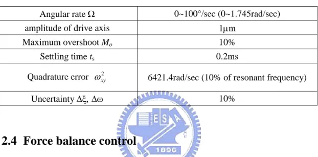
(32) (a) f0=10071Hz. (b) f0=10100Hz. (c) f0=10220Hz. (d) f0=10344Hz. Fig. 2.6 Modal analysis (a) mode1, (b) mode2, (c) mode3, (d) mode4. The lumped and operation parameters of the system are shown in Table 2.1. Simulink was used to simulate the dynamic response of the system and the performance of the controller. System specifications are shown in Table 2.2. The amplitude of the drive axis is controlled at 1um, and the sense axis is assumed to be static. The maximum angular rate to be measured is 100°/sec. The allowed variation of the system parameters to be considered in this thesis is 10%. The settling time is 0.2ms and the maximum overshoot is 10%.. 21.

(33) Table 2.1 System parameters Structure thickness. 100µm. Capacitance gap. 4.5µm. Quality factor Q. 450. Resonant frequency f (ω) Equivalent mass. 10220Hz (64214rad/sec) 1.251×10-6kg. Damping coefficient ξ. 1.11×10-3. Table 2.2 System specifications Angular rate Ω. 0~100°/sec (0~1.745rad/sec). amplitude of drive axis. 1µm. Maximum overshoot Mo. 10%. Settling time ts. 0.2ms. Quadrature error ω xy2. 6421.4rad/sec (10% of resonant frequency). Uncertainty ∆ξ, ∆ω. 10%. 2.4 Force balance control The concept of the force balance is often applied to the control of inertial sensors. Coriolis force is considered as a disturbance in the governing equation. The controller is designed to provide a feedback force to counteract the Coriolis force and the quadrature error to maintain the displacement of the sense axis at zero. Therefore, the coupled system can be modeled as two systems with the coupling viewed as disturbance, as shown in Fig. 2.7. The reference inputs of the two axes are 10-6sinωt and zero, respectively. The controller will be designed according to the loops in Fig. 2.7.. 22.

(34) 〈Drive axis〉 10-6sin ωt. −ω xy2 y + 2Ωy +. K. Resonant frequency. Fx +. +. xˆ. Plant. −. +. + n. −ω xy2 x + 2Ωx. 〈Sense axis〉 Σ. K. Fy +. +. yˆ. Plant. −. +. Demodulator. + n ˆ Ω. Fig. 2.7 Control loop of two axes. 2.5 Demodulation The rotation rate can be obtained through demodulation. In this thesis, the displacement of the sense axis is maintained at zero by a feedback force to cancel the Coriolis force and quadrature error terms from the drive axis. The normalized force can be expressed as: Fy u y = =−ω xy2 x − 2Ωx m. (2.8). The angular rate Ω and the quadrature error ω xy2 can be derived by demodulating the feedback force uy. If the displacement x of the drive axis is represented by a sinusoidal signal x = Asinωt, the angular rate Ω can be demodulated from the feedback force uy by the multiplication by cosωt:. 23.

(35) u y ⋅ cos ωt = ( −ω xy2 x − 2Ωx ) ⋅ cos ωt =−ω xy2 A sin ωt cos ωt − 2ΩAω cos 2 ωt. (2.9). 1 = − ω xy2 A sin 2ωt − ΩAω cos 2ωt − ΩAω 2. 1 In Eq. 2.9, the high frequency signals − ω xy2 A sin 2ωt and −ΩAω cos 2ωt can be 2 filtered out by a low pass filter (LPF). Therefore, the angular rate Ω can be found from:.  u y ⋅ cos ωt  = Ω FLPF  − , Aω  . (2.10). where FLPF ( ⋅) represents the function of a low pass filter. In the same way, the quadrature error ω xy2 can be demodulated from the feedback force uy by the multiplication of sinωt:.  2u ⋅ sin ωt  = ωxy2 FLPF  − y  A  . (2.11). A second order filter attenuates higher frequencies more steeply than a first order filter. The transfer function of the filter is. FLPF ( s ) =. 1. (τ s + 1). (2.12). 2. where τ is a time constant. The rolloff is 40 dB per decade at high frequency. Because the resonant frequency is about 10000Hz, the time constant τ of the low pass filter is chosen as 1×10-4, so that the high frequency (2ω) signals are attenuated by 12 dB.. 2.6 Summary In this chapter, the operating principle of the micro vibrating ring gyroscope, source and effects of system variation, and system parameters are presented. 24.

(36) Closed-loop control is used in this research. The displacement of the drive axis is to be controlled at the constant amplitude of 1µm; the displacement of the sense axis is to be maintained at zero. A feedback force is used to counteract the disturbance caused by Coriolis force and quadrature error. The angular rate Ω can be derived by demodulating the feedback force. The controller design will be discussed in Chapter 3.. 25.

(37) Chapter 3. Controller design. The objectives of this research are to eliminate disturbance and to deal with parameter uncertainty. PID control is a general industrial control method and the QFT/H∞ control is a robust control method. These two methods are used to design the controllers in this chapter. The performances of these two controllers are compared by Simulink system in Chapter 4.. 3.1 System analysis In Chapter 2, the governing equations of the MEMS gyroscope and the system parameters were presented. From Eq. 2.4 and Table 2.1, the uncoupled transfer functions of the two axes are as follows: = G (s). 1m 7.99 ×105 = s 2 + 2ζω s + ω 2 s 2 + 142.7 s + 4.123 ×109. (3.1). In this section, the characteristics of the transfer function in time domain and frequency domain are discussed.. 3.1.1 Characteristics in time domain If the Coriolis force is considered as an internal disturbance of the system, the government equation of the gyroscope can be decoupled to two independent transfer functions for the two axes, as shown in Eq. 3.1. For this standard second order system with the natural frequency ω = 64214 rad / sec and damping coefficient ξ = 1 900 , the maximum overshoot Mo and settling time ts of the step response are [19]: −πξ 1−ξ = M o e= 99.65% 2. = ts. (3.2). 4.6 = 0.064sec. ξω. 26.

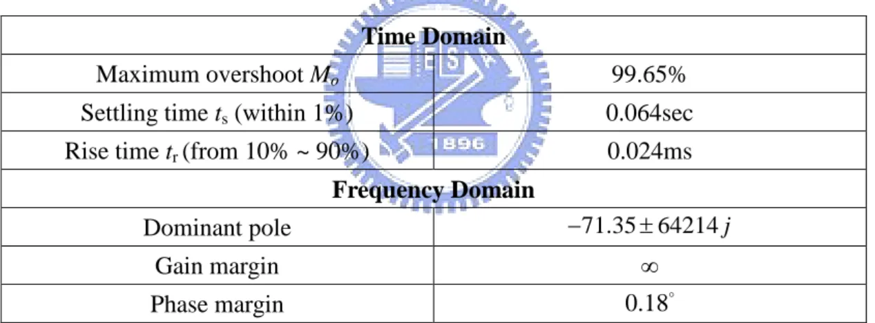
(38) The MATLAB simulation of the step response of the plant is shown in Fig. 3.1. From Eq. 3.2 and Fig. 3.1, the maximum overshoot is too large and the settling time of the open-loop system is too long. Therefore, a controller is needed to improve the transient response performance. The characteristic in frequency domain is listed in Table 3.1.. Fig. 3.1 Step response of MEMS gyroscope. 3.1.2 Characteristics in frequency domain In frequency domain, the dominant poles of the uncoupled transfer function Eq. 3.1 are derived as −71.35 ± 64214 j . The Bode plot is shown in Fig. 3.2. The original gain margin is infinite, and the phase margin is only 0.18°. If the gyroscope is operated in resonant frequency, it will have the largest amplitude and the drive voltage can be reduced. The characteristic in frequency domain is also listed in Table 3.1.. 27.

(39) Fig. 3.2 Bode plot of MEMS gyroscope plant. Table 3.1 Characteristics in time and frequency domains Time Domain Maximum overshoot Mo. 99.65%. Settling time ts (within 1%). 0.064sec. Rise time tr (from 10% ~ 90%). 0.024ms. Frequency Domain Dominant pole. −71.35 ± 64214 j. Gain margin. ∞ 0.18°. Phase margin. 3.2 PID control design using pole placement A proportional–integral–derivative (PID) controller is a generic control loop feedback mechanism widely used in industrial control systems. A PID controller attempts to correct the error between a measured variable and a desired set-point by calculating and then outputting a corrective action. The controller can be design by moving the poles to the new locations to satisfy the specifications.. 28.

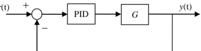
(40) 3.2.1 PID controller Once the transfer function of the system is derived, the corresponding PID controller can be designed. The schematic of the closed-loop system with the PID controller is shown in Fig. 3.3.. r(t). +. y(t). PID. G. −. Fig. 3.3 Schematic of the closed-loop system with a PID controller. The PID controller includes three parameters: the Proportional, the Integral and the Derivative gains. The Proportional gain determines the reaction to current error, the Integral gain determines the reaction based on the sum of plant errors and the Derivative gain determines the reaction to the rate at which the error has been changing. The transfer function of a PID controller is.   K 1 + Td s  = K p + i + K d s Gc ( s ) = K p 1 + s  Ti s . (3.3). where Kp is the proportional gain, K i = K p Ti is the integral gain, and K d = K pTd is the derivative gain. Because the specifications have been defined, the PID controller can be designed by pole placement [20] to move the poles to the appropriate place to satisfy the specifications.. 3.2.2 Pole placement method Pole placement is one of the control methods to make the system satisfy the specifications by moving the poles of the system to the appropriate places. In a closed-loop system, the pole placement has a direct effect on time response, such as 29.

(41) rise time, settling time, maximum overshoot, etc.. The design starts with an assumption of what form the controller must take in order to control the given plant. Typically, specifications lead to the formation of a second order equation. Most of the final characteristic equation will have more than 2 poles, and additional desired poles must be determined. Algebra is used to determine the controller coefficients necessary to achieve the desired closed-loop poles with the assumed controller form. Typically, an integrator is used to drive the steady-state error towards zero. This implies that the final characteristic equation will have at least one more pole than uncontrolled system.. 3.2.3 Using pole placement to design PID controller From Eqs. 3.1 and 3.3, the characteristic equation of the closed-loop system with a PID controller, 1+GcG = 0, can be expressed as:. (s. ). (. ). 1 K d s 2 + K p s + Ki m 1 1 1     = s 3 +  2ξωn + K d  s 2 +  ω 2 + K p  s + K i m m m     Φ CL =. 2. + 2ξω s + ω 2 s +. (3.4). The desired characteristic equation is determined by the maximum overshoot and settling time in the specifications. Because there are three poles in Eq 3.4, it can be expressed as. 2 ( s + a ) ( s 2 + 2ξdesiredωdesired s + ωdesired ). , where a is an extra pole.. Comparing the coefficients of the desired characteristic equation with the closed-loop characteristic equation Eq. 3.4, the PID gains can be solved. In the time domain specifications, the maximum overshoot is 10% and the settling time is 0.2ms. So the desired damping coefficient ξdesired is 0.591 and the desired natural frequency ωdesired is 38300rad/sec from Eq.3.2. The extra pole is supposed to be at ten times of the natural frequency. But it was found in simulation that such an extra pole would make the closed-loop system unstable. Therefore, the 30.

(42) extra pole was placed at 1000x of the natural frequency, a = −3.83 × 107 . The desired characteristic equation of the closed-loop can be expressed as:. (. ) (. 2 Φ CL =  s 2 + 45194 s + 3.83 ×104  s + 3.83 ×107  . ). (3.5). The three gain parameters of the PID controller can be obtained by comparing Eq. 3.5 with Eq. 3.4, as listed in Table 3.2.. Table 3.2 PID controller gain Result Kp. 418.6. Ki. 1.363×107. Kd. 9.3×10-3. PID. 9.3 ×10−3 s 2 + 418.6 s + 1.363 ×107 Gc ( s ) = s. 3.3 QFT/H∞ Control Both Quantitative Feedback Theory (QFT) and H∞ design techniques have be developed for a long time [21]. The QFT and H∞ design techniques are popular robust feedback control schemes which can achieve the desired system objectives no matter if there is any uncertainty. In this thesis, the two methods will be applied to design the controller. The standard schematic of the closed-loop system by QFT/H∞ design method is shown in Fig. 3.4.. r(t). F. +. e. K. u. −. G. +. +. d y(t). +. + n. Fig. 3.4 Schematic of the general closed-loop system with QFT/H∞ controller. 31.

(43) 3.3.1 QFT design technique QFT was first introduced by Horowitz and Sidi [21]. This method translates the time domain specification to the frequency domain and uses Nichols Chart to find the boundary conditions. It also makes the system output satisfy the desired specifications by moving the poles and the zeros of the controller to the suitable positions. The general problem is how to design the controller K and prefilter F in Fig. 3.4. Fig. 3.4 is a two degrees of freedom (TDOF) feedback system, which includes plant P, controller K, prefilter F, input signal r, output signal y, disturbance d, and sensor noise n. The controller K is the first design degree of freedom used to reduce system sensitivity from disturbance and noise. The prefilter F is the second design degree-of-freedom used to satisfy the required performance. Thus the plant output is bounded and constrained by the given specifications. Two boundary conditions in time domain, Bu and Bl, are given, so that the output y(t) is bounded by:. Bl ( t ) ≤ y ( t ) ≤ Bu ( t ). (3.6). These tracking specifications in the time domain are translated into the frequency domain as the upper bound and the lower bound, as shown in Fig. 3.5,. Bl (ω ) ≤ T ( jω ) ≤ Bu (ω ). (3.7). where. Y (s) = T= ( s ) F ( s ) T1 ( s ) R (s) F ( s ) is a prefilter, and T1 ( s ) =. K (s)G (s). 1+ K (s)G (s). (3.8). is the loop gain.. Because the QFT theory is part of the robust control design, the sensitivity is the most important factor in studying the parameter variation effect. The definition of 32.

(44) sensitivity specification is expressed as [17]:. SGT ( s ) ≡. ∂T T ∆T T ≅ or ∂G G ∆G G. SGT ( s ) ≡. ∆ T ( jω ) max. ∆ G ( jω ) max. (3.9). where ∆ T ( jω ) max and ∆ G ( jω ) max are the maximum variation of T ( jω ) and. G ( jω ) , which is 10% in this thesis. In the QFT theory, the upper bound is an under damped system, ξ < 1 , and the lower bound is an over damped system, ξ > 1 . Thus, the specifications in time domain can be applied to set the upper bound and the lower bound conditions. With the given boundary condition, Nichols Chart is applied to design the controller. In this thesis, the controller is designed by H∞ method. The prefilter F(s) will move the closed loop gain T1(s) to within the upper bound and the lower bound, as shows in Fig. 3.5, to fit the specifications by adding poles and zeros.. Fig. 3.5 Unity feedback closed-loop for different plant cases [17]. 3.3.2 H∞ control method [22] The H∞ control method is applied to design a robust controller when system parameters change or disturbance exists. In the H∞ control theory, as shown in Fig. 3.6, K is the controller and G is the generalized plant including the plant and the weighting 33.

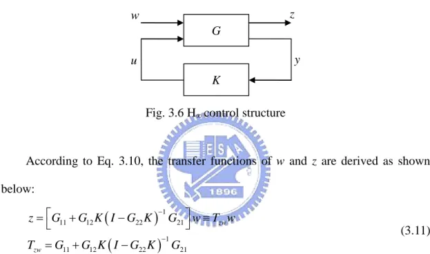
(45) functions. It can be written as:. z   w   G11 G12   w  = = G y  u  G G  u       21  22  . (3.10). where w is a vector signal including noises, disturbances, and reference signals, z is a vector signal including all controlled signals and tracking errors, u is the control signal, y is the measurement.. z. w G. y. u K Fig. 3.6 H∞ control structure. According to Eq. 3.10, the transfer functions of w and z are derived as shown below: G11 + G12 K ( I − G22 K )−1 G21  w ≡ Tzw w z=   Tzw =+ G11 G12 K ( I − G22 K ) G21 −1. (3.11). where Tzw is transfer matrix of w to z. The purpose of H∞ control is to design a controller K to suppress the controlled value z. The magnitude of Tzw is defined by the H∞ norm and can be expressed as:. Tzw. ∞. = supω σ {Tzw ( jω )}. (3.12). where σ ( ⋅) means the maximum singular value, and sup ( ⋅) means supremum or least upper bound, and is defined as the smallest real number that is greater than or equal to this number. It is the maximum value of the gain in the Bode plot, and the maximum distance to the origin in the vector diagram. According to the input signal and the output signal shown in Fig. 3.6, the H∞ norm of Tzw can be redefined as 34.

(46) Tzw ( s ). ∞. = supω. z w. 2. (3.13). 2. From Eq. 3.13, it can be observed that the problem of H∞ control is to minimize the transfer matrix of w to z in the form of H∞ norm, and satisfy. Tzw ( s ). ∞. <γ ,. which γ is the chosen positive number.. 3.3.3 Combined QFT/H∞ control The combined QFT/H∞ control method does not use the Nichols Chart to design the controller. Instead, the controller K is first calculated by the H∞ optimization control method, and then the prifilter F is added to make the output fit the performance requirement. The design steps are shown in Fig. 3.7, where the most important part of the design is to transfer the specifications of the system into appropriate weighting functions. Step 1 is finding out the weighting function, and translating into the H∞ control structure as shown in Fig. 3.6. Step 2 is using H∞ method to calculate controller K, and using the boundary condition to define prefilter F. The closed-loop system with the controller K can be stabilized by minimizing the sensitivity and the disturbance w can have the minimal effect on the expectable output z. A function D(ω) is given to specify the disturbance rejection specifications, and the sensitivity function has satisfied S ( jω ) ≤ D (ω ) . The sensitivity function is constrained to satisfy this inequality W1 ( jω ) S ( jω ) ≤ 1 , where the weighting function W1 is used to limit the sensitivity function and can be chosen by W1 ( jω ) ≤. D (ω ). S ( jω ). .. 35.

(47) 〈Step 1〉 r1. +. e. u +. K. d. +. y. G. −. +. z3. W2. W1 + −. + n. z2. z1. r1. + Specification. K. e. +. +. W3. d. y. G. u. +. + n. z. w G. Use H∞ method to calculate K. y. u K 〈Step 2〉 r. F. r1. +. e. K. u +. +. d. −. G. y. +. + n. Fig. 3.7 QFT/H∞ design step. The sensor noise amplification is not expected to exist in high frequency. If the high sensor noise amplification can be reduced, the cost of feedback design can be also reduced. After given nominal plant G0, the transfer function from noise n to controller output u is Tun=. u −K . It stands for the amplifier effect of the sensor = n 1 + KG0. noise. The weighting function W2 has to satisfy W2 ( jω ) Tun ( jω ) ≤ 1 . A good control system should have proper loop-gain, which reduces the sensor noise at high. 36.

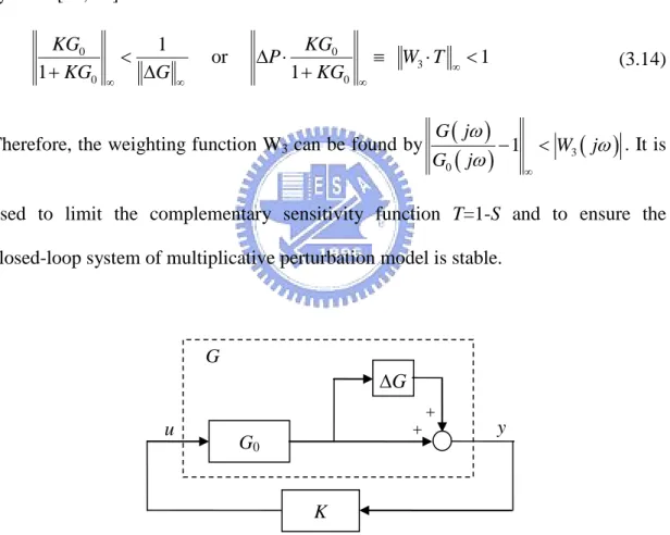
(48) frequency. This property is considered in choosing W2 and W1. It is found practical and efficient here to use the control weighting function W2 as a tuning parameter in optimization process. Considering the parameter variations, if the multiplicative perturbation modeling structure of the plant is used [17], as shown in Fig. 3.8, then G can be represented by. = G G0 ( I + ∆G ) , where ∆G is the error of multiplicative model. This structure allows the modeling of various plant uncertainties, and the condition for stable closed-loop systems [22, 23] is. KG0 1 + KG0. < ∞. 1 ∆G. or. ∆P ⋅. ∞. KG0 1 + KG0. ≡ W3 ⋅ T. ∞. <1. (3.14). ∞. Therefore, the weighting function W3 can be found by. G ( jω ). G0 ( jω ). − 1 < W3 ( jω ) . It is ∞. used to limit the complementary sensitivity function T=1-S and to ensure the closed-loop system of multiplicative perturbation model is stable.. G. ∆G u. +. G0. +. y. K Fig. 3.8 Multiplicative perturbation model of the plant. In short, the three weighting functions satisfying Eq. 3.15 are necessary and sufficient for the solution of the proposed QFT/H∞ design technique.. 37.

(49) W1 ( jω ) S ( jω ) ∞ ≤ 1 W2 ( jω ) Tun ( jω ) ∞ ≤ 1. (3.15). W3 ( jω ) T ( jω ) ∞ ≤ 1. 3.3.4 Design of QFT/H∞ controller for MEMS gyroscope The flow chart of the QFT/H∞ design method is shown in Fig. 3.9. First, the settling time and maximum overshoot specifications are applied to define the upper bound and lower bound. The upper bound uses the specifications to calculate that the damping coefficient ξ = 0.59 and natural frequency ωn = 38301. Since the lower bound is an over damped system, the damping coefficient is assumed as ξ = 1.1, and the natural frequency is shown as ωn = 20543. The two bounds are defined as B ( s )= ωn2. (s. 2. + 2ξω s + ωn2. ). and can be expressed as:. 1.467 ×109 s 2 + 45194 s + 1.467 ×109 4.22 ×108 Bl ( s ) = 2 s + 45194 s + 4.22 ×108 Bu ( s ) =. (3.16). To relax the restrictions in high frequency and to maintain the system performances, the pole (s+3.83×105) to the lower bound and the zero (s+2.05×105) to the upper bound are added. The two bounds become. s   1.467 ×109 1 + 5   3.83 ×10  Bu ( s ) = 2 s + 46194s + 1.467 ×109 4.22 ×108 Bl ( s ) = ( s 2 + 46194s + 4.22 ×108 ) 1 + 2.05s×105 . (3.17). The three weighting functions of the plant are found by Eq. 3.15 and Fig. 3.9,. s 2 + 1.018 ×108 s + 3.142 ×1013 W1 ( s ) = 70128s 2 + 140.26 s + 0.0701 W2 ( s ) = 0.1 W2 ( s ) = 39 38. (3.18).

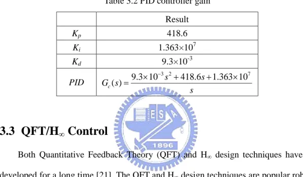
(50) After the weighting functions are found, the “hinflmi” instruction in MATLAB is used to solve for the LMI-based H∞ controller. The prefilter F is then added to adjust the frequency response so that it completely lies between the upper bound and the lower bound. The controller and the prefilter are as follows:. K (s) =. 1.885 ×1010 ( s + 28.34)( s 2 + 2.324 ×104 s + 4.121×109 ) ( s + 0.02)( s + 0.0014)( s 2 + 6.875 ×105 s + 1.193 ×1011 ). 0.132 (s+2.5 ×105 ) (s+2 ×105 ) F (s) = (s+6 × 104 ) (s+5 ×104 ). Problem specifications Translate Tu(t),Tl(t) Tu( ω), Tl(ω). Obtain W3 for robust stability Fix initial W2, calculate sensitivity S and resolve W1. Find the controller K by H∞ method. Modify W2. No.  T1 ( jω ) max ≤ ∆ T1 ( jω ) max. Yes. bound. Refinement of the. Design prefilter F. design if necessary. Evaluation of design. End. Fig. 3.9 Flow chart of combined QFT/H∞ design. 39. (3.19).

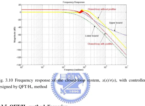
(51) The frequency response of the system with controller and prefilter is shown in Fig. 3.10. The red solid lines are the response of the family of plants with 10% variation in natural frequency and damping coefficient, as described in section 2.3.. Fig. 3.10 Frequency response of the closed-loop system, x(s)/r(s), with controller designed by QFT/H∞ method. 3.3.5 QFT/H∞ method discussion The QFT/H∞ control method discussed above is different from conventional QFT/H∞ control in a number of aspect. In this thesis, the Coriolis force and the quadrature error are regarded as inner disturbances of the system before the plant, as shown in Fig. 3.7. But in standard QFT/H∞ control method, the disturbances are after the plant, as shown in Fig. 3.4. Therefore, the way of deriving the weighting functions needs to be modified.. 3.4 Summary A PID controller and a QFT/H∞ controller are designed according the same. 40.

(52) specifications. The former is the general control method and can be easily realized. The latter is a robust controller over fabrication errors and model uncertainties. The simulation results with the two controllers and the robustness comparison are presented in Chapter 4.. 41.

(53) Chapter 4. Simulation and Discussion. This Chapter presents the Simulink simulation of the open-loop system, the PID control, QFT/H∞ control, and comparison with other publications. The reference position of the drive mode has an amplitude of 1µm at the resonance of 64214 rad/sec. The angular rate 100°/sec is added to the system at t = 0.1sec. The Simulink model of the plant is shown in Fig. 4.1. All the simulation is with double precision of 10-14.. (b). (a). (c). Fig. 4.1 Simulink model of the gyroscope (a) overview (b) detail of Subsystem for drive axis (c) detail of Subsystem for sense axis. 4.1 Open-loop system The governing equation of the drive axis can be rewritten as:. (. Fx = mx + bx + kx = m  x + 2ξω x + ω 2 x. ). (4.1). The desired trajectory of the drive axis is x = A sin ωt , x = Aω cos ωt and  x = − Aω 2 sin ωt , where A = 1×10-6m. The other parameters can be found in Table 2.1.. In the ideal case, the drive force to drive the displacement of the drive axis at 1µm at. Fx 1.15 ×10−5 cos 64214t N. The the resonant frequency can be found from Eq. 4.1 as= Coriolis force from sense axis is ignored in the calculation because the displacement 42.

(54) of the drive axis is much larger than the displacement of the sense axis. Because the displacement of the sense axis is to be maintained at zero, the reference input of the sense axis is zero. For an open-loop system, only the Coriolis force acts on the sense axis. The governing equation of the sense axis can be expressed as:. (. Fy =−2mΩx =my + by + ky =m  y + 2ξω y + ω 2 y. ). (4.2). With Ω = 100°/sec and other parameters from Table 2.1, Eq. 4.2, becomes:. (. ). −2.8 ×10−7 cos ( 64214t ) 1.251×10−6 y + 142.7 y + 4.123 ×109 y =. (4.3). The differential equation can be solved and the displacement of the sense axis is. −2.44 ×10−8 sin ( 64214t ) m. found as y =. 4.1.1 Model verification Fx 1.15 ×10−5 cos 64214t N, can be used to The force derived from Eq. 4.1, = drive the lumped model Eq. 2.1, which has a quality factor Q = 450, to a displacement of 1µm at resonance. However, the same force, when applied to finite element modeling, will cause a displacement larger than that allowed by the spring structures outside the vibrating ring due to a much larger quality factor in the numerical calculation.. Therefore,. the. force. is. reduced. by. a. factor. of. 100. to. = Fx′ 1.15 ×10−7 cos 64214t N before it is used in the finite element modeling to verify the lumped model. As shown in Fig. 4.2, a pair of sinusoidal forces Fx′ in opposite directions are exerted on the ring in the direction of the drive axis. The deformation of the structure at resonance is shown in Fig. 4.3. As shown in Fig. 4.4, the maximum displacement of x = 4.32µm occurs at f = 10220.37Hz, which is the same as that used in the lumped model. The displacement at low frequency is 4.3×10-5µm. The quality factor of the system in the simulation can be derived as 1×105. 43.