ELSEVIER Journal of Crystal Growth 171 (1997) 601-613
j . . . C R Y S T A L G R O W T H
Assessment of mathematical models for the flow in directional
solidification
Jay W. Lu, Falin Chen *
Institute of Applied Mechanics, National Taiwan Unil,ersiO', Taipei 10764, Taiwan, ROC
Received 19 January 1996; accepted 7 May 1996
Abstract
In a binary solution unidirectionally solidified from below, the bulk melt and the eutectic solid is separated by a dendritic mushy zone. The mathematical formulation governing the fluid motion shall thus consist of the equations in the bulk melt and the mushy zone and the associated boundary conditions. In the bulk melt, assuming that the melt is a Newtonian fluid, the governing equations are the continuity equation, the Navier-Stokes equations, the heat conservation equation, and the solute conservation equation. In the mushy layer, however, the formulation of the momentum equation and the associated boundary conditions are diversified in previous investigations. In this paper, we discuss three mathematical models, which had been previously applied to study the flow induced by the solidification of binary solutions cooling from below. The assessment is given on the bases of the stability characteristics of the convective flow and the comparison between the numerical and experimental results.
1. Introduction
Directional solidification is a processing tech- nique with which many of the advanced metals, such as the gas turbine blade, are manufactured. The resultant casting consists of long columnar crystals oriented roughly in the direction of the thermal gradient, showing increased creep rupture strain and improved thermal fatigue behaviour [1]. During the directional solidification process, the planar freezing front is morphologically unstable and the solidifica- tion is dendritic [2]. Dendrites grow highly convo- lutely, generating a melt/solid interface of a very large specific area. As a result, from a macroscopic point of view, the melt is separated from the solid by
* Corresponding author.
a region consisting of solid dendrites and interden- dritic liquid, referred to as a dendritic mushy zone.
Owing to solidification, convection evolves, start- ing from salt-finger convection to plume convection as well as large-scale convection in the bulk melt [3]. Convection influences the metallic structure and is also responsible for the macrosegregation of the casting. The characteristics of the convective flows have attracted a large research efforts in the past three decades; see, for example, the review papers by Davis [4] and Huppert [5]. To describe the fluid motion in directional solidification, mathematical formulations are developed for both the bulk fluid and the mushy regions. In each region, governing equations essentially consist of the conservation of mass, momentum, energy and concentration(s). As the melt is assumed to be a Newtonian fluid (as it 0022-0248/97/$17.00 Copyright © 1997 Published by Elsevier Science B.V. All rights reserved
602 J.W. Lu, F. Chen /Journal of Crystal Growth 171 (1997) 601-613
used to be), the momentum equation in the bulk fluid is the incompressible Navier-Stokes equation and the energy and concentration conservation equations are formulated according to the Fourier law. In the mushy region, however, the mathematical approach is more complex. To which, in fact, most of the research efforts had been devoted. Regarding the system of binary solution cooling from below, the development of the mathematical model is briefly described in the following.
Hills, Loper and Roberts [6] systematically devel- oped a full set of thermodynamic equations for a mushy region, while solving a much-reduced one-di- mensional set to approximately analyze the growth of a binary alloy. In their analysis, the growth of mush was assumed to advance with a prescribed constant velocity. To release this growth-constrain- ing assumption, Huppert and Worster [7] formulated a simpler mathematical model on the basis of global conservation relations. The model turns out to be easier to use than that developed by Hills et al. [6], while the assumption that the solid fraction is con- stant throughout the mush eliminates the possible interaction between convection and solidification. Worster [8] improved this model by considering the solid fraction as a function of space and time, lead- ing to a qualitative description of the morphology of the mush. His model is closed by including a marginal-equilibrium condition at the melt/mush in- terface. Unlike the above mathematical models in which no buoyancy-induced convection is consid- ered, Fowler [9], based on the thermodynamic rela- tions developed by Hills et al. [6] and employed the Darcy law to be the momentum conservation in the mush, was able to analyze the convective stability in the mush. Using Fowler's model in the mush as well as the common model in the bulk melt, several investigations [10-12] have successfully analyzed the stability characteristics of the convective flow in the directional solidification system in which a den- dritic mushy layer underlying a semi-infinite bulk fluid layer is considered. Their numerical results were confirmed by experiments [12-15].
The above models treat the mushy and the bulk fluid regions separately, which usually require ex- plicitly tracking the melt/mush interface of regular shape as well as incorporating empirical relations between the solid fraction and the permeability of
the mush. To avoid these constrains, a so-called single-domain model was developed by Beckermann and Viskanta [16], based on the volume-averaging approach and also by Bennon and Incropera [17] based on the mixture-theory approach. Both ap- proaches result in a single-set of equations, including again the momentum equation as well as the equa- tions concerning the conservation of mass, energy and concentration. This set of equations applies in all three regions (bulk fluid, mush, and solid regions) in the directional solidification system. The interfaces of melt/mush and mush/solid as well as individual phase variables are treated implicitly. As a result, generally, except the momentum equation is different from that of the models mentioned previously, all other equations in both the fluid and the mushy layers are essentially the same. The momentum equa- tion for the single-domain approach in fact is equiva- lent to the Brinkman-extended Darcy law, which differs from the Darcy equation mainly by the vis- cous diffusion term as well as the nonlinear advec- tion term. As a result, mathematically, the multi-do- main model shall be equivalent to the single-domain model as the Brinkman-extended Darcy equation is employed as the momentum equation in the mushy layer.
In the present paper, the multi-domain approach is employed to assess the mathematical models that had been used to analyze the convective flow in direc- tional solidification of binary solutions. The first model to be considered is that used by Worster [10] and Chert, Lu and Yang [12], in which the Darcy equation is employed as the momentum equation in the mushy layer and the Navier-Stokes equation as the momentum equation in the fluid layer, and non- slip boundary condition is prescribed at the melt/mush interface. It is noted that the formulation of the multi-domain approach involves mathemati- cally the coupling of the Navier-Stokes equation with the Darcy equation through an appropriate set of matching conditions at the melt/mush interface. The two momentum equations are of different order of differentiation, necessitating the use of some form of empirical conditions. Worster [10] employed the non-slip condition based on the assumption that the characteristic length scale of the flow on the melt/mush interface is much larger than the space between the arms of the dendrite. This, in general
J.w. Lu. F. Chen / Journal of Crystal Growth 171 (1997) 601-613
603 sense, however, may not be the case since theboundary-layer mode convection (to be discussed in Section 3.1) prevails in the system for most of the cases observed in the experiments [3,12]. An alterna- tive was proposed by Beavers and Joseph [18] who systematically developed an empirical condition be- tween the horizontal velocities of the fluid and the porous layers (or a homogeneous and isotropic mushy layer) with a series of experiment. This condition primarily allows a slip between the velocities above and below the m e l t / m u s h interface. The validity of this condition was confirmed by Taylor [19] and Saffman [20] with respectively an analytical and a statistical approach. Numerical evidences have also been provided by Neale and Nader [21], Beavers, Sparrow and Masha [22], Nield [23], and so on. We therefore replace the non-slip condition with the Beavers-Joseph condition such that the second mathematical model is formed. The third model would be that the momentum equation in the mush is the Brinkman-extended Darcy equation, associated with the continuities of the velocities and the first derivative of velocities across the m e l t / m u s h inter- face. This model is mathematically equivalent to the model developed with the single-domain approach.
These three models cover virtually all the mathe- matical approaches presently used in the analysis of the directional solidification of binary solutions. The assessment will be made on the bases of the dynamic features of the onset of the convective flow, the comparison with the experimental results, the valid- ity of the model relevant to the observed convective flows, and so on. The details of the mathematical formulation for the three models are described in Section 2. The numerical results in terms of neutral curve topology, the criteria of stability and the criti- cal flow patterns, and the comparison with the exper- imental results, are given in Section 3. The assess- ment and discussion on the three models as well as the conclusion are given in Section 4.
2 . M a t h e m a t i c a l f o r m u l a t i o n
The details of the three mathematical models are described in this section. Since most of the equations for the three models are the same, we will illustrate the details of the first model and only indicate the part different from the other two models.
2.1. Model 1
We illustrate first the mathematical model consid- ered by Worster [10], which is supposed to be the simplest model of the three models considered. For the convenience of subsequent discussion, the details of the mathematical formulation of this model are described in the following.
Consider a mushy layer that lies above a eutectic solid region and below a semi-infinite fluid region. A binary solution of concentration C~ and temperature T-s_ is unidirectionally solidified from below. Both the melt/mush and mush/solid interfaces move up- wards with a constant velocity V. The mushy layer extends from z = 0 to z =
h(x,y,t),
where x, y and z are the three axes of Cartesian coordinate, t is time, and h is the position of the m e l t / m u s h inter- face to be determined as part of the solution. In such a system, two sets of equations and three sets of boundary conditions at respectively z = 0, z = h and z = zc are required to describe the fluid motion as well as the heat and mass transfer in the system.We non-dimensionalize the fluid velocities with the interface velocity V, distances with
K J V ,
time with Ktl/V 2, and pressure with /3A C p o g K J V ;
in which Ktl is the thermal diffusivity of the fluid, / 3 = / 3 " - F o l * , /3" and a * the solutal and ther- mal expansion coefficients, respectively, F the slope of the liquidus curve, which is assumed to be a constant, AC = C~ - C E, C E the eutectic concentra- tion, P0 a reference density, and g the gravitational acceleration constant. By assuming that the physical properties of the fluid and solid are identical [ l 0] and by taking the Galilean transformation with respect to the moving interface, we obtain the following dimen- sionless equations. In the fluid layer h < z < zc, we have V ' u = O , - - - 0 + u • V 0 = V 2 0 , Ot~ - -~z O + u " 7 0 = eV20'
o" -~t + u V u= V2U + R T O e k - Rc(O)ek + ~ , VP),
(2) (3) (4)6 0 4 J.W. Lu, F. Chen/Journal of Crystal Growth 171 (1997)601-613
where u = ( u , v , w ) is the velocity vector. The dimen- sionless temperature and concentration are defined as
T - TL(C~) C - C,
0 -
AT
, O= A---U-'
(5)
where A T = F A C = TL(C ~) -TE,TL(C~) is the liq- uidus temperature corresponding to C~, • = Kc]/Ktl the Lewis number, Kc] the solutal diffusivity of the fluid, o-= V/Ktl the Prandtl number, e~ the unit vector in the vertical direction, p the pressure, R T and R c the thermal and solutal Rayleigh numbers given by
gol * A TH 3 g ~ * A C H 3
R T - , R c , (6)
Ktl b' Ktl b'
in which v is the kinematic viscosity and H the characteristics length. In the mushy-layer 0 < z < h, we have v . , , = o, (7) at Oz O + u " VO= V z O - g - ~t - X, (8) X - - ~ z O + u . V O = - ( O - ~ ) 0 t - 0 z X, (9) U Rm(V p + 0ek), (10)
/7( x)
where X is the porosity, / 7 ( X ) the dimensionless permeability function of X, ~ = (C~ - C:¢)/AC the concentration ratio, C~ the concentration of solid,
o ~ - = . ~ / c A T the Stefan number, ~ the latent heat
of fusion, c the specific heat, and R m the Rayleigh
number for the mushy layer given by
g ~ A C / 7 o H
R m - - , (11)
K t l / ~
in which /7o is the reference permeability. Note that since the thermodynamics equilibrium condition holds in the mushy layer [12], the liquidus relation 0 = O is applied in the mushy layer. The solute diffusion in the mush is so small that the • in the mush is assumed to be zero for the time being. This
assumption will be justified by the discussion of Section 3.4.
The boundary conditions at the z ~ ~ are
0--, (12a)
0 --, o, (12b)
u ~ O, (12c)
at the m e l t / m u s h interface z = h are
0 = O, (13a) n- V 0 = n . VO, (13b)
[ . - . ] =o,
(13c)
[0] =o,
(13d)
[ n - V 0 ] = 0 , (13e) X = 1, (13f) [ p ] = 0 , (13g)u-(n.u)n=O,
(13h)where the square brackets denote the jump of the enclosed quantity across the interface and n a unit vector normal to the interface. In the above boundary conditions, Eq. (13a) is the liquidus relation, Eq. (13b) the marginal equilibrium condition [8], Eq. (13c) the continuity of normal velocity, Eqs. (13d) and (13e) the continuities of temperature and heat flux, respectively, Eq. (13f) an enforced condition assuming the solid at the interface vanishes, Eq. (13g) the continuity of normal stress, and Eq. (13h) the non-slip boundary condition employed by Worster [10]. At the mush/solid interface z = 0 we have
0 = - 1, (14a)
w = 0, (14b)
since the temperature here is assumed to be the eutectic temperature T E and due to viscosity the non-penetration condition at the solid boundary is satisfied.
2.2. Model 2
The equations and associated boundary conditions of model 2 are the same as those of model 1 except that the non-slip boundary condition at the m e l t / m u s h interface (Eq. (13h)) shall be replaced by
J.W. Lu, F. Chen /Journal of Crystal Growth 171 (1997) 601-613 605 the Beavers-Joseph condition, which can be written
in dimensionless form as
OU2
/= A V
(15)
where /./2 accounts for the horizontal velocity vector
(u,t:), H ( I ) the permeability at the melt/mush inter-
face, A an empirical constant determined experimen- tally, which is assumed to be 0.1 for the present case [24], A~ "J = H2/IIo the inverse of the Darcy number,
and H the characteristic length. Eq. (15) in essence means that at the m e l t / m u s h interface a " s l i p " between the velocities in the fluid and the mushy layer is proportional to the shear rate. By replacing Eq. (13h) with Eq. (15), model 2 is closed, with a less restrictive condition at the m e l t / m u s h interface.
2.3. model 3
The momentum equation in the mushy layer of model 3 is the Brinkman-extended Darcy law, which can be written as
l
)1
+ - ( u . V
u
cr at 32 X[u
1
= v
-
(16)
u / / ( x )Eq. (16) differs from the Darcy law (Eq. (10)) by the unsteady term and the nonlinear term on the left- hand-side and by the second-order differential term on the right-hand-side. The use of the Brinkman-ex- tended Darcy law, as discussed by Walker and Homsy [25] and Nield [23], is important when the porosity of the mushy layer is large, which can be true for some materials of high entropy production upon solidifica- tion [26]. By employing Eq. (16) as the momentum equation in the mushy layer, the matching conditions regarding the flow velocities shall include the conti- nuities of the velocities and the first-order deriva- tives of the velocities, replacing Eqs. (13c) and (13h) of model 1.
2.4. Basic state
The above three models differs mainly from the momentum equation in the mushy layer and the
associated boundary conditions at the m e l t / m u s h interface. The motionless basic state accordingly shall be the same for all models. The equations and asso- ciated boundary conditions shown above admit a motionless steady solution, which is a function of z. In the fluid layer, as u vanishes, Eqs. (2) and (3) become respectively
- O ' b = 0 ' ~ , ( 1 7 )
- o ; =
where the index b accounts for the basic state and ' for the vertical derivative d / d z . By solving the above equations with the relevant boundary condi- tions, the basic state temperature and concentration are obtained as
0 b = 0~ + ( 0 i - 0:~)e - ( ' - h ) . (19)
O h = 0 i e (" h ) / e (20)
and the interfacial temperature given by E
0 i - - 0r. (21)
In the mushy layer, the relation of thermodynamic equilibrium 0 = 69 applies [12]. The basic state equa- tions can be deduced from Eqs. (8) and (9) as
- 0 b = 0~ + . Y - X b , ( 2 2 )
--gb0b = ( 0b -- g~) Xb" (23)
The above two equations with the relevant boundary conditions can be deduced further to obtain
~ - 0 i
Xb -- - - (24)
~ - 0 b
0 b =.Y-(I - Xb) + 0~ -- 0 b, (25) where Eq. (25) can be solved with a shooting tech- nique.
2.5. Linear stabilio, equations
We linearize the equations of the three models by introducing small disturbances to the basic state quantities of Section 2.4 and substituting their com- bination into the original equations. After obtaining the linearized equations by neglecting higher-order terms of disturbance quantities and applying the normal modes proportional to e x p ( w t + i a x ) , the
606 J. W. Lu, F. Chen / Journal of Co'stal Growth 171 (1997)601-613
small disturbance equations are obtained as follows. In the fluid layer, we have
( D 2 - a Z ) w = / 2 , (26)
( D 2 + D - w - o~2)0 =
O'bW,
(27) ( e D 2 + D - t o - e a z ) 6 1 =61'b W,
(28)( o o )
D 2 + - a 21 2 = a 2 ( R v O - R c 6 1 ) .
(29)o-
In these equations, the notations W, 0, 61 now represent small disturbance quantities. In addition, both ' and D represent the vertical derivative d / d z, a the horizontal wavenumber, to the normal mode frequency, and 1 2 = - V X V × u . Note that the Rayleigh numbers in the fluid can be replaced by the Rayleigh number in the mush by the relations R T =
A~UR m
and R c = ( 1 + A ) ~ Rm,
where ~Z/'=H2/Ho,
H = / ( , 1 / g , and A =Fa */fl
is the buoy- ancy ratio between the buoyancy due to temperature to that due to concentration.For model 1, through the same procedure of linearization, the linearized equations in the mushy layer can be obtained as follows:
( D 2 + D - a 2 -
t o ) O + 9 - ( D -
t o ) X =ObW,
(30)
[Xb(D-to)+Xb]0
+ [ O b + ( O b - - g O ( D - - t o ) ] X = O b W,
(31)[ D2
II'(Xb)
]
~ b ) D - a 2 W = a2ff/( )(b)Rm0. (32) Note that in Eq. (31) the liquidus relation 0 = O has been applied.The boundary conditions at z ~ ~ are
0 = 0, (33a) 69 = 0, (33b) W = 0, (33c)
DW
= 0, (33d) at z = h are 0 = 6t, (34a) [ l - E ~ ,DO - DO = ~ ----~-- ) Ob r/,
(34b) [W ] = O, (34c) [ 0 ] = 0 ,[DO] -
~ - - 0 io;
x -
r/'
DWb, + = O,
D Wb, -
m r / ,
(34d) (34e) (34f) (34g)[
,
U(l) D12+--(12+ 2w-toDw)
o-- 2 a 2 D W 1 ,
(34h) Jh + and at z = 0 a r e 0 = 0, (35a) W = O, (35b)where 7/ is the small perturbation of the interface position.
For model 2, the non-slip boundary condition Eq. (34g) shall be replaced by the linearized Beavers- Joseph condition
o2wlh+=a
T (DWI,,+-DWIh ).
(36)
For model 3, the linearized momentum equation in the mushy layer isD212 - ( )('b Xb O" 1) D12
1
- ~ / / ( + o- Xb + +--o- 12 + 2{d)(bH
X.) + --o" Xb DW
a2 X;
W = - a 2YX b R m 0, (37) o- Xbwhich shall replace Eq. (32) of model 1. The associ- ated boundary conditions at m e l t / m u s h interface at z = h are
[DW]
= 0 ,[ a ] =o,
DOlh÷ = [ D O - - -
t
(38a) (38b) U ( 1 )DW
,
(38c) .I hJ.W. Lu, F. Chert~Journal of Co'stal Growth 171 (1997)601-613 6 0 7
to replace Eqs. (34g) and (34h) of model 1. An additional condition at z = 0,
DW = 0, (39)
shall be included for model 3 to meet the require- ment due to the additional two orders of differentia- tion in the momentum equation Eq. (37).
2.6. Method ¢~f solution
The equations and the associated boundary condi- tions of each model consist a complex eigenvalue problem
F(Rm,ce,w; 0~, ~ , ~ ' , g , Y , tr, e,/-I ) = 0 (40) in which a set ordinary differential equations of
totally thirteen-order of differentiation of models 1 and 2 and fifteen-order of model 3 subject to rele- vant boundary conditions are to be solved numeri- cally. Note that the boundary condition Eq. (34b) is employed to compute the perturbed interface posi- tion r/.
We solve these eigenvalue problems with a shoot- ing technique, in which the integration is imple- mented in a truncated domain [27] and the far-field boundary conditions Eqs. (33a)-(33d) are imposed at a sufficiently large distance, which is taken to be 20 for the present study, so that the integrations are independent of the value of the truncated distance. Note that in the mushy layer the basic state is known only implicitly, a change of independent variable proposed by Worster [10] is used to avoid the need
200 1 5 0 1% 100 50 (a)
/:///'//:"
~ " - ~ I ,' I d l I I o 50 40 30 CO 20 10 0 5 10 15 20 25 30 200 150 R,, 100 50 (b) 50 40 30 20 10 0 5 10 15 20 25 30 C~ 200 1 5 0 R,, 100 50 (c) 5 0 4 0 3 0....::
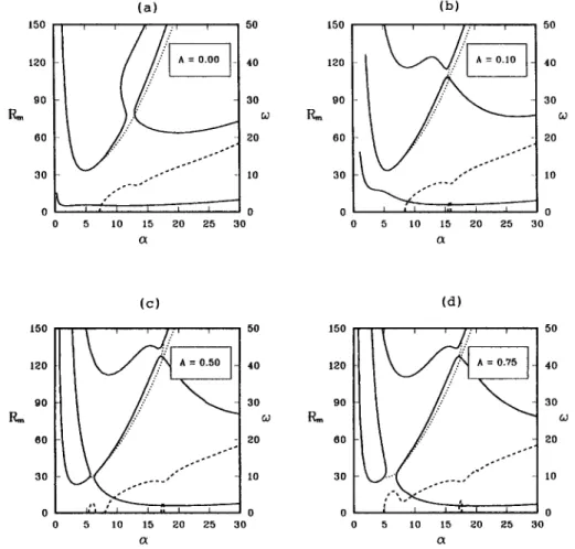
2O A 0 5 0 I0 I : l t ;' l l 0 5 10 15 20 25 30 200 150 w P~ aoo 50 (d) o o 50 40 3O 6o 20 10 0 5 IO 15 20 25 30 F i g . 1. N e u t r a l c u r v e s o f m o d e l 1 f o r v a r i o u s ,a¢ o f t h e c a s e 0~ = , Y - = ~ = 1, ~ = 0 . 0 2 5 , o - = 10, ~ ' = 105, a n d H = 1, r e l e v a n t to an a q u e o u s s o l u t i o n . (a) , a ¢ = 0; ( b ) ~ = 0.1; ( c ) L~" = 0.5; (d) . a ¢ = 0.75. ( ) C o n v e c t i o n o f s t e a d y onset. ( . . . ) C o n v e c t i o n o f o s c i l l a t o r y onset. ( - - - ) V a l u e o f w.608 J. W. Lu, F. Chen / Journal of Crystal Growth 171 (1997)601-613
to invert the transcendental equation. The final equa- tions are solved by a so-called superposition method developed by Keller [28], in which an orthonormal- ization is imposed to avoid the loss of linear inde- pendence of integration. An iteration procedure de- veloped by Powell [29] is employed to seek the convergence of the eigenvalues R m and w.
3. Numerical results
We consider an alloy of o-= 10, E = 0.025, ~ = J = 0~ = 1, ~ = 105, and a uniform permeability / 7 = 1, which is relevant to the aqueous solution [10]. Special attention will be paid to the parameter ~¢, or the buoyancy ratio, accounting for the ratio between the buoyancy due to thermal expansion to
that due to solutal expansion. Physically, the value of represents the involvement of the interaction be- tween thermal and solutal gradients, or the intensity of double-diffusivity. As a result, ~¢ is influential on the characteristics of the convective stability in terms of both the convection mode as well as the critical condition [12]. Accordingly, changing ~¢ may serve as a good indicator for the assessment of the mathe- matical models, based on both the stability character- istics as well as the dynamic features of the onset of convection.
3.1. The neutral curve topology
We first examine the neutral curves, which may reflect the dynamic features of the onset of the convective flow. Fig. 1 shows the results from model
150 120 90 60 30 0
(a)
.-" 10 ' - - I J' I I ~ 0 5 I0 15 20 25 30 C( 50 40 3O 20 1 5 0120
90 60 30 0(b)
, , .., , 50 3 0 0 20 0 5 10 15 20 25 30 1% 150 120 90 60 30 0 (c) i i :::, i 5 tO 15 20 25 C( 50 150 4 0 120 30 90 20 60 tO 30 0 0 3O ( d ) , , :, , 50' ~ ~
40
30 J i i '* i { o 5I0 15
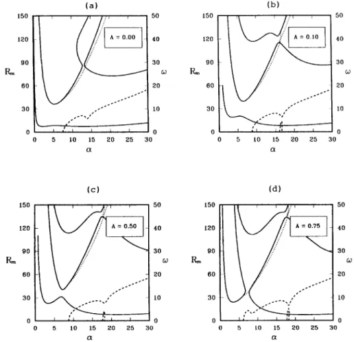
20 25 30 aFig. 2. Neutral c u r v e s o f model 2 for various za¢ o f the case 0~ = 3 - = ~ = 1, E = 0.025, o - = 10, Y = 105, a n d 1 7 = 1, relevant to an
a q u e o u s solution. (a) ~ ' = 0; (b) ~a¢= 0.1; (c) :a ¢ = 0.5; (d) J = 0.75. ( ) C o n v e c t i o n o f steady onset. ( . . • ) C o n v e c t i o n o f
J. W. Lu. F. Chen / Journal of Crystal Growth 171 (1997) 601-613 609
1 for , ~ varying from 0 to 0.75. For ~ = 0 (Fig. l a), the three marginal curves (solid curves) representing the convection of steady onset and the two (dotted curves) representing the convection of oscillatory onset consist the neutral curve map. In the same figure, the dashed curve represents the value of ~o, or the frequency of oscillation, corresponding to the oscillatory mode. The lowest solid curve is bimodal, in which the mode of smaller wavenumber c~ is more unstable. This mode is called the mushy-layer mode (MLM) since the convection circulates be- tween the mushy layer and the fluid layer, being of a length scale about the height of the mushy layer. The solid curve at the middle is also bimodal, in which the mode of smaller c~ is more unstable. For the oscillatory mode, the lower dotted curve emerges
from the middle solid curve, penetrating into the domain enclosed by the middle and the upper solid curves, ends near the bottom of the upper solid curve. The upper dotted curve emerges from the upper solid curve and goes upwards with increasing c~. It is noted that the frequency w in general in- creases with o~ except near the transition of changing one mode into another.
As ,~/increases to 0.1 (Fig. lb), the lowest solid curve is also bimodal while the mode of larger ce becomes more unstable. Since the convection of this mode is largely confined to the solutal boundary layer above the m e l t / m u s h interface, it thus is called the boundary-layer mode (BLM) convection. For the middle solid curve, nevertheless, the M L M is still more unstable. As ,e' increases further, the solid
(a) (b) 150 , , , . ~ , 50 150 50 120 ...:/':[ A -- O.O0 40 120 40 P,,m 9060 I _ ~ /6 ~0 1 ~ ' - 3020 ' " 9060 3020 60
31 ~
010
300
otO
0 5 I0 15 ~ 0 25 30 0 5 tO 15 20 25 30 150 120 90 P~ 6 0 30 (c) 50 150 40 I2030
90
2060
10
30
' "' ' :! ~ ' 0 05 10 15
ZO25 30
G
(d) 5o 4o 3o 2o [o o5 tO 15 20 Z5 30
Fig. 3. Neutral curves of model 3 for various ,~ of the case Oh =,~- = ~','= 1, • = 0.025. o-= 10, ~f = 105, and H = 1. relevant to an aqueous solution. (a) ,~g= 0; (b) ,a¢= 0.1: (c) ,&= 0.5; (d) L¢= 0.75. ( - - ) Convection of steady onset. (. - . ) Convection of oscillatory onset. (---) Value of ~o.
6 1 0 J. W. Lu, F. Chen / Journal of Cr3,stal Growth 171 (1997) 601-613 Rm 5 0 4 0 3 0 2 0 10 0 (a) i l p : i i 2 : I I i k I 5 10 15 2 0 2 5 3 0 LX ( b ) 5 0 , , 40 • [ i ] ]
a0
i
i
]
Ro
:
i
Model :1 , 0 2 5 10 15 2 0 2 5 3 0 C(Fig. 4. S u m m a r y of the lowest solid (monotonic) curves o f the
three models considered. ( a ) . a e = 0; ( b ) o ~ ' = 0.1.
curves m o v e closer, see Fig. l c for a / = 0.5. Eventu- ally, see Fig. ld for a d = 0.75, the solid curves become two groups, one on the left and one on the right, representing respectively the MLM branch and the BLM branch. A Hopf bifurcation branch (dotted curve) connects the two monotonic branches (solid curves). Another oscillatory branch with higher fre- quency emerges from the upper part of the fight-hand branch and ends at the same branch. Also shown in the same figure is a third oscillatory branch emerg- ing from the upper part of the left-hand branch, its corresponding frequency increases monotonically with o~. The occurrence of the Hopf bifurcation branch, more precisely at oq = 0.69, may be impor- tant to the subsequent plume convection, which will be discussed in Section 4.
For model 2 (Fig. 2), the neutral curves look similar to those of model 1. The MLM also domi- nates the lowest monotonic curve at ,~¢ = 0 and the BLM becomes dominant as , ~ > 0. The Hopf bifur- cation branch appears at , ~ = 0.47, which is much lower than model 1. For model 3 (Fig. 3), the neutral curves are also similar to those of previous two models while the Hopf bifurcation occurs at ,~¢= 0.64.
3.2. The critical conditions
To experimenters, the lowest R m, or R~,, is the most meaningful value since at which the onset of
Ro= 12 (a) : i M o d e l 1 : 3 0 (b) Model 1 C ~ c 2 0 ! 0 . . . . . : . . . : • , . . . . • J 0 I 0 . 0 0 0 . 1 5 0 . 3 0 0 . 4 5 0 . 6 0 0 . 7 5 0 . 0 0 0 . 1 5 0 . 3 0 0 . 4 5 A A
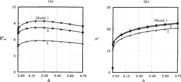
Fig. 5. Comparison of ( a ) R~, a n d ( b ) a c resulted from the three models for .U/varying from 0 to 0 . 7 5 .
J. W. Lu, F. Chen / Journal of Crystal Growth 171 (1997) 601-613 611 convection occurs. The corresponding onset flow
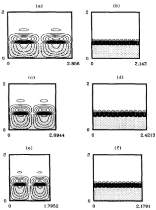
pattern, or the critical flow pattern, can be the flow to be seen in the experiment. W e therefore show in this section the comparison of the R~ resulted from the three models and their corresponding critical flow patterns. Fig. 4 summarizes the lowest mono- tonic curves o f the three models for o~¢ = 0 and 0.1. For , ~ = 0 (Fig. 4a), results from all models show that the most critical mode is invariably the M L M , the R~ of model 2 is the smallest and that of model 1 is the largest. For ~¢ = 0.1 (Fig. 4b), all models lead to the same result that the BLM dominates the convection and, again, the R~ of model 2 is the smallest and that o f model 1 is the largest. Fig. 5 shows all the R~ and the corresponding a ~ for all , ~ o f the three models, illustrating that the R~ of model 2 is the smallest for all o~/considered while those of model 1 is the largest. Note that the influ- ence of ~¢ on the stability o f convection is complex in the present system, on which an intensive discus- sion has been provided by Chen, Lu and Yang [12]. Fig. 6 shows the critical flow patterns of , ~ = 0.1. It is found that the B L M essentially is a convection cell sitting above the m e l t / m u s h interface and the M L M consists two separated cells, one in the mushy layer and one in the fluid layer, viscously coupling in the vicinity of the interface. The critical flow pat- terns from different models are similar except that the critical wavelength differs from one to another. W e also examine the flow patterns corresponding to the first occurrence o f the H o p f bifurcation, namely, at ,a¢ = 0.69 for model 1, ~ = 0.47 for model 2, and , ~ = 0.64 for model 3, and find that they all look similar to the M L M , consisting o f two separated cells while having a smaller wavelength.
3.3. Comparison with experiment
Tait and Jaupart (1989) conducted an experiment and showed that the onset of convection in a 28% NH4CI aqueous solution unidirectionally solidified from below occurs at R~, = 8. From their experimen- tal conditions we can deduce the following parame- ters o - = 10, e = 0.013, ,a¢ = 0.65, 3 - = 2.43, ~ = 8.675, 0~ = 0.144, and ~ = 3.48 × 10 6. Based on the above parameters we compute the R~, for the three models and find that the neutral curves resulted from the three models are very similar. Difference,
(a)
10
o 0 2.856 (b) 2 0 2 . 1 4 2 (c) 2 0 0 0 2 . 0 9 4 4 (e) 2 o o 1 . 7 9 5 2 (d) 2 ::::::::::::::::::::::::::::::::::::::::::::::::::::::::::::::::: ,....H.,. • ;.:.:.:,:.:.:.:.:. / .:.:.:.:.:.:.:.:.:.: :.:.;.:,:.:.:,:.:.: : 0 . . . " ' ' . . . ' . . . 0 2 . 4 2 1 3 (f) 2 0 2 . 1 7 9 1Fig. 6. The critical flow patterns resulted from the three models. (a) Model l, MLM. a < = 3.42, R m = 18.896: (b) model 1, BLM, a ~=17.6, Rm=9.140; (c) model 2, MLM, a c=3.00, Rm= 18.530: (d) model 2, BLM, a ~ = 15.5, R,, = 5.653: (e) model 3, MLM, a c = 3.50, R m = 18.855; (f) model 3. BLM, o~ c = 17.3, R m = 8.047. The shadow accounts for the mushy layer. The horizontal dimension of each figure is scaled with respect to the mushy-layer height.
however, is observable from the value of R~, where the R~, o f model 1 is 11.091, of model 2 is 8.455, and of model 3 is 10.613. The above R~, all corre- sponding to the BLM, lie within a satisfactory range comparing with the experiment while model 2 results in the closest R~ to the experiment.
3.4. Solutal d~ffusir, i ~ in the mush
It is mentioned in Section 2 that the solutal diffu- sivity in the mush is assumed to have vanished since it can be very small in reality. To confirm this, we consider the solute diffusivity in the mush by adding the term eV2~9 into Eq. (9) and by e m p l o y i n g model 2 as the benchmark model for tests. W e compute the neutral curves for the four different .~¢ considered in
612 J.W. Lu, F. Chen /Journal of Crystal Growth 171 (1997) 601-613
Figs. 1-3 and compare with Fig. 2. Results show that the addition of the solutal diffusivity in the mushy layer indeed does not lead to any significant difference in terms of numerical result. But, nonethe- less, it causes an increase of the computing time by about twice since, as will be discussed in Section 4, this term causes a stiffness problem. We thus would suggest that the negligence of the solutal diffusivity in the mush is essential to the present system.
4. Discussion and conclusion
The above results show that model 2, Darcy law in the mush associated with the Beavers-Joseph slip condition at the interface, leads to the smallest R c, which is the closest to the experimental result. On the other hand, the R~ of model 1 is the largest, reflecting that the non-slip condition prescribed at the m e l t / m u s h interface may be slightly more re- strictive. The Brinkman extension of the Darcy law applying in the mushy layer essentially does not lead to any significant difference since the convective flow velocity in the mush is indeed very small.
It is known from previous investigations [10-12] that the stability characteristics of the onset of con- vection has a close relation with the subsequent plume convection of the system. More precisely, the plume convection, a liquid plume carrying cooler and less concentrated fluid emerges from the interior of the mushy layer and penetrates into the fluid layer above, can be either a result of a subcritical MLM under the strong perturbation of the nonlinear BLM or a direct result of the critical MLM. The stability characteristics of the plume convection in the nonlin- ear regime shall be studied by the mathematical models considered in the present paper. In fact, investigations [30,31] have been devoted to the com- putation of the plume convection with the single-do- main approach, or equivalently model 3. The results of the present study show, however, that model 2 can be a better approach for pursuing the nonlinear sta- bility analysis. The reasons are as follows. Model 2 results in both a smallest R e as well as a smallest d for the occurrence of Hopf bifurcation, implying that the nonlinear computation can be more easily pur- sued since a wider range of R m c a n be considered and the Hopf bifurcation can be studied under a
smaller ~ . Moreover, both smaller R m and smaller oa¢ give a less restrictive condition for the numerical stability such that a converged solution can be ob- tained with less computer time.
Regarding the computation efficiency, according to the present linear stability analysis, the computer time needed for running through a case of model 3 is more than three times of either model 1 or 2. This is due to the fact that the momentum equation in the mushy layer of model 3 is two orders of differentia- tion higher than the other two models. The additional term ~,V2u causes a stiffness problem because its quantity is generally much smaller than the other terms in the same equation; which is similar to the case of Section 3.4 considering the solutal diffusion in the mushy layer. Since the present results show that this term does indeed lead to insignificant differ- ence compared to the other models, the use of model 3 can be redundant for the present system. However, model 3 may be necessary when the permeability of the mushy-layer is significantly large [23,25], while it can not be the case in most of the metallic system [32].
The computational efficiency for models I and 2 are quite similar, while the programming of model I is relatively much easier since the use of the non-slip boundary condition is more straight forward than that of the Beavers-Joseph condition. However, as mentioned previously, the non-slip condition may impose a too restrictive condition on the interface, leading to a higher R~I. On the other hand, the Beavers-Joseph condition is developed under a sys- tematic approach, and has been confirmed both nu- merically and experimentally by several investiga- tions. We thus suggest that model 2 shall be the most suitable mathematical model for the directional solid- ification of binary solution, which in brief is easier to use and leads to a more reasonable result.
The above conclusions are made on the basis of the results obtained for a particular set of parameters shown at the beginning of Section 3 and a range of ,a¢, and shall be valid for a different set of parameters in the practical sense. The reasons are as follows. The three models differ mainly from the momentum equations in the mush a n d / o r the corresponding boundary conditions at the m e l t / m u s h interface. As the BLM prevails, the fluid in the mush is virtually quiescent and, accordingly, the model difference shall
,I.W. Lu, F. Chen /Journal of Co'stal Growth 171 (1997) 601-613 613
not lead to any significant change of the above conclusions. Discussions of Chen, Lu and Yang [12] regarding the influence of these parameters suggest that the BLM occurs in a wide range of parameters relevant to most of both the aqueous solutions and the metallic solutions. Although the MLM can pre- dominate the system as ~ is small (or the perme- ability is large), this possibility, nevertheless, shall be excluded in the practical sense because, first, most of the X resulted from metallic casting [32] or aqueous solution [15] are not so small, and secondly, for a small We the Darcy equation is no longer valid in the mush [25] and model 3 shall be the only choice valid lbr the analysis.
Acknowledgements
The financial support for this work from Nation Science Council through Grant No NSC 85-2212-E- 002-010 is gratefully acknowledged.
References
[1] M. McLean, Directionally Solidified Materials for High Temperature Service (The Metals Society, London, 1983). [2] W.W. Mullin and R.F. Sekerka, J. Appl. Phys. 35 (1964)
444.
[3] C.F. Chen and F. Chen, J. Fluid Mech. 227 (1991) 567. [4] S.H. Davis, J. Fluid Mech. 212 (1990) 241.
[5] H.E. Huppert, J. Fluid Mech. 212 (1990) 209.
[6] R.N. Hills, D.E. Loper and P.H. Roberts, Q. J. Mech. Appl. Math. 36 (1983) 505.
[7] H.E. Huppert and M.G. Worster, Nature 314 (1985) 703. [8] M.G. Worster, J. Fluid Mech. 167 (1986) 481.
[9] A.C. Fowler, IMA J. Appl. Math. 35 (1985) 159. [10] M.G. Worster, J. Fluid Mech. 237 (1992) 649.
[11] G. Amberg and G.M. Homsy, J. Fluid Mech. 252 (1993) 79. [12] F. Chen, J.W. Lu and T.L. Yang, J. Fluid Mech. 276 (1994)
163.
[13] S. Tait and C. Jaupart, Nature 338 (1989) 571. [14] S. Tait and C. Jaupart, J. Geophys. Res. 97 (1992) 6735. [15] C.F. Chen, J. Fluid Mech. 293 (1995) 81.
[16] C. Beckermann and R. Viskanta, Physico Chem. Hydrodyn. 10 (1988) 195.
[17] W.D. Bennon and F.P. Incropera, Int. J. Heat Mass Transfer 30 (1987) 2161.
[18] G.S. Beavers and D.D. Joseph, J. Fluid Mech. 30 (1968) 197. [19] G.I. Taylor, J. Fluid Mech. 49 (1971) 319.
[20] P.G. Saffman, St. Appl. Math. 50 (1971) 93.
[21] G. Neale and W. Nader, Can. J. Chem. Eng. 52 (1974) 475. [22] G.S. Beavers, E.M. Sparrow and B.A. Masha, AIChE J. 20
(1974) 596.
[23] D.A. Nield, J. Fluid Mech. 128 (1983) 37. [24] F. Chen, J. Appl. Phys. 71 (1992) 5222.
[25] K. Walker and G.M. Homsy, J. Heat Transfer, ASME 99 (1977) 338.
[26] M. Copley, A.F. Giamei, S.M. Johnson and M.F. Hom- becker, Met. Trans. 1 (1970) 2193.
[27] S.R. Coriell, M.R. Cordes, W,J. Boettinger and R.F. Sekerka, J. Crystal Growth 49 (1980) 13.
[28] H.B. Keller, Numerical Solutions of Two Points Boundary Value Problems, Regional Conference Series in Applied Math. (SIAM, Philadelphia, PA, 1976).
[29] M.J.D. Powell, Numerical Methods for Nonlinear Algebraic Equations, Ed. P.H. Rabinowitz (Gordon & Breach, London, 1970).
[30] S.D. Felicelli, J.C. Heinrich and D.R. Poirier, Met. Trans. B 22B (1991) 847.
[31] D.G. Neilson and F.P. lncropera, Int. J. Heat Mass Transfer 34 (1991) 1717.