A new generation of evaluation tool for online design and scheduling in an advanced manufacturing system

(1)

Proceedings of the 1999 EEE

International Conference on Robotics & Automation Detroit, Michigan May 1999

A

New Generation of Evaluation Tool for On-Line Design and

Scheduling in An Advanced Manufacturing System

Ming-Hung Lin and Li-Chen Fu

Dept. of Computer Science and Information Engineering

National Taiwan University,Taipei,Taiwan,R.O.

C

E-mail: lichen@ccms.

nt u. edu. tw

Abstract

In business, new product development is the name of the game. An efficient evaluation tool is cru- cial. This paper proposes a new generation of evaluation tool for on-line design and scheduling, wherein planned control policy designed by engineers will be on-line evaluated. Performance will be evaluated by a new prediction rule that differs from existent state- independent or steady state model such as a queuing network model. In addition to that, a new optimal control rule or schedule can then be derived from the original planned ones and the feedback from the manufacturing engineers. Simulation and prediction methods are applied together t o give an optimum in the timeslot of snapshot. Such evaluation tool can also be used t o look for the possible conflicts in the potential solution and suggest some necessary steps t o avoid those conflicts.

1 Introduction

A manufacturing system in today’s environment usually has thousands of interrelated variables. The manufacturing systems need not only some negative feedback t o keep the enterprise stable when there is a market for them but also some positive feedback to make the systems adaptable t o the market. Tradi- tional flexible manufacturing systems - management and evaluation methods based on hierarchical control [6]

-

are unable to meet the requirements in such a complex environment. Instead, we need a new evaluation support system based on self-organization prin- ciple, i.e., an interactive system with self-learning and self-adaptive capabilities.

The rule for measuring the performance is called performance prediction rule. In general, consideration of performance assignment is an important element in the life cycle of production. The queuing theory has been taken as the starting point for such prediction rules [l] [2] [3]. However, queuing net-

work analyzer can only give the average performance

over a relatively long period of time. But the performance of manufacturing nowadays usually focuses on a short term to quickly respond t o the drastically changing market place. Owing t o this, a new prediction rule is needed which differs from existent state- independent or steady state model such as a queuing network model.

As we all know, most of the scheduling, planning, or layout problem, for example, will require resolution by employing such kind of algorithms. However, if the criteria is represented in analytic form, then the problems at hand will become NP-hard problem. This situation can be alleviated by means of simulation. The joint use of simulation models and optimization methods has been widely studied [4]. Those methods are in the use of the data obtained from the previ- ous simulation to find a new starting point that is close to the global optimum. However, it is not fast enough to meet the changing speed of environment. The area about performance prediction supporting decision making in job-shop production has been proposed [7], but it was limited and just gave conceptual description. The originality of the method in the arti- cle is to make use of the data generated by prediction

as the direction t o find the optimum. According t o that, it will be very efficient to respond to the change of the manufacturing environment.

Nowadays, in the complicated real word, it is important to consider more than one objective simulta- neously when engineers making decision due t o the surrounding complexity [5]. However, the objectives of interest are usually in conflict with one another. Although one objective can be improved, other objectives might be degraded a lot. We proposed a method called negotiation net to support engineers t o integrate various kinds of objectives objectives and information effectively. This method also finds the possible conflicts in the potential solution and some necessary steps to avoid the conflicts.

The organization of the paper is as follows. In the next section, we will state the problem and give some discussions. In section 3, an on-line operation model

(2)

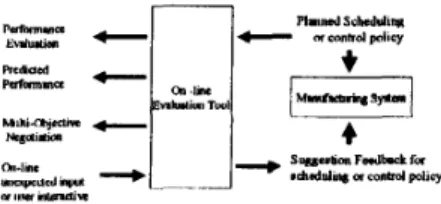
Figure 1: The evaluation tool

for the proposed evaluation tool. Besides that, the prediction diagnosis together with the optimal feedback using simulation and prediction will also be ad-

dressed. In section 4,the proposed evaluation tool is implemented based on a robotic flexible assembly cell, where the proposed tool is tested via a number of simulation. In section 5, a brief conclusion is made.

2 Problem Statement and Analysis

The evaluation tool is a complete developing envi-

1, that was defined to solve ronment shown in Fig.

the following questions:

(1) How to obtain a better solution derived from the original planned one and to have on-line feedback to manufacturing engineers.

(2) How to measure performance and to give an op-

timal performance evaluation or prediction, and how to support engineers for evaluation so that it is to integrate many engineers' objectives and information effectively.

2.1 Performance Prediction

Given a set of classes of jobs, let M be the total

number of classes and Ni be the number of job for the

ith class. We denote the j t h job in the ith class as

j o b i j . The rule of performance measure is called performance prediction rule, and the consideration of performance assignment is an important element in the life cycle of production. Let Pt be a prediction rule generated at time t , then the state-dependent predic-

tion process can be formulated as follows:

pt = Z [ X ( t ) , P t - I , (1)

where Pt- is the precedence of the prediction rule at time t - , X ( t ) is the state variable at time t , and 2

is denoted as a prediction diagnosis function. Let

D$,(Pt) be the qth predicted performance of job ij with control policy R

,

and control policy R is to be evaluated with the proposed evaluation tool

.

Let the qth performance of jobij at the end be denoted as

Cij,(R), then our objective is to minimize the root- square value of variation V i ( P t ) for the qth predicted performance defined as

i j

and V i ( P t ) is also denoted as the prediction variation of pt *

2.2 Feedback for Control Policy

Let Rack be a new control policy generated by the evaluation tool. Consider the ratio U ( R ) , which is defined as

where the control policy R is the original planned one to be evaluated, q is denoted as performance, e.g., throughput, tardiness, and U,(R) is also denoted as the gain of feedback

.

The problem of feedback for control policy can be mathematically stated as:

max U, ( R )

-+

min

B

subject to

Rack E HR

HR = {Rack

I

%(Rack)

5

fi,

I

= 172, ' ' * S},

where gi and fi are constraints. The objective is then

to find a Rack belonging to the set of admissible so-

lution HR which minimizes the criteria U , ( R ) . The optimization conduction problem F can be formulated

as follows:

(4) where we define Po as an optimal prediction rule such that W(V'(Po)) is a minimization and W ( . ) is the ex- pected value operator. Y is a set of simulation data,

Y = E ( U i j j o b i j ) , and E is an approximated input function, i.e., random distribution, normal distribution.

F(Rack, Y, Po) --+ min,

2.3 Multiple Objective

For easy illustration, considering the due-date as- signment

D

= a

+

PP

+

y N , where a , D , P , N are the arrival time, assigned due-date, total processing- time and the required number of operations of a job, respectively; /3 and y are the respective processing- time and the number of operation multiples. Then, D

(3)

is the objective which will be considered, and we denote a , P, N as characteristic variables(CV). Let D be

denoted as the objective of requirement(0R). In gen- eral, there is a relationship matrix M which illustrates the relationship between every characteristic variable and every objective of requirement. Suppose we know that CVs have effect on every OR. The data Mij in the relationship matrix stands for a certain contribu- tion of Cvi t o ORj. From a different viewpoint, data Mij means the probability of a certain CV’s contribu- tion to the satisfaction of a certain ORj. No matter what, the value of Mij may be positive or negative, which means that CVs will obstruct or increase a certain ORi. The value Mij is also a common random variable, which is a well known distribution with a mean value mij. Let R be a planned control policy

to be evaluated by the evaluation tool. We denote the impact function of characteristic variables as

ai,

CV, = @i(R), which means the value of CK is affected by R. Thus, a multi-objective optimization problem can be formulated as

where

i

Here, R* is called a completed feasible solution if there exists no other feasible solution R E

D R

such that

foRj(R)

5

foRj(R*) for all i = l , . . . , N . Consider an associated multi-objective problem from f (R) for

a list of weighting parameter a1,.

,

_a~:

(7)

where

ciai

= 1. Then, our goal is t o verify Mij to

avoid conflict solution

,

to decide which ai should be urgently improved and t o maximize the Equation (7).

3 The On-line Operation Model

of

Evaluation Tool

3.1 The On-line Operation Model

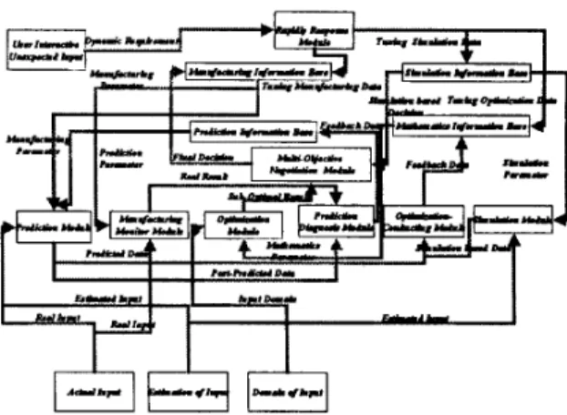
The block diagram of on-line operation model for proposed evaluation tool can be presented in Fig. 2.

The components of the on-line operation model are described in the following.

Manufacturing Monitor Module: This is an entity

that is t o monitor the status of tasks or machines. This module gets the manufacturing information from the Manufacturing Information Base.

Figure 2: The block diagram of on-line operation

model

Rapidly Response Module: This module handles

on-line data such as the interaction from users or unexpected inputs from the environment. It will take the snapshot of on-line manufacturing data; all of prediction module, optimization module and simulation module depend on the snapshot of on-line data.

Prediction Module: This module takes over the

performance evaluation. It has two inputs that are actual on-line manufacturing data and approximated manufacturing data. There are two types of performance evaluation, namely, pre-

dicted data and post-predicted data. If the input data are approximated, then the results of performance evaluation belong t o predicted data. On the other hand, if the input data are actually manufacturing data, then the results belong to

post-predicted data whiles using the same predic-

tion rule. This module takes the current manufac- turing parameter from Manufacturing Informa-

tion Base and parameter of prediction rule from Prediction Information Base.

Optimization Module: In this module, the criteria

of manufacturing problem is represented in analytic form. An optimal solution will be obtained derived from the original planned scheduling or control policies. This module takes the control parameter from Mathematics Information Base.

Simulation Module: This module performs the

simulation before each stage of planned control policy is issued. This module takes the simulation parameter from Simulation Information Base.

(4)

Figure 3: The diagnosis of prediction rule

Figure 4: The use of simulation and prediction for optimization

Prediction Diagnosis Module: The process of pre-

diction diagnosis module is presented generally in Fig. 3. The details of this process can be

described in sub-section 3.2.

Optimization Conducting Module: The process of

optimization conducting module is presented generally in Fig. 4. The details of this process can be described in sub-section 3.3.

The process of multi-objective negotiation module is presented generally in Fig. 5. The details of this process can be described in sub-section 3.4.

Multi-objective Negotiation Module:

3.2 General Approach for Operation

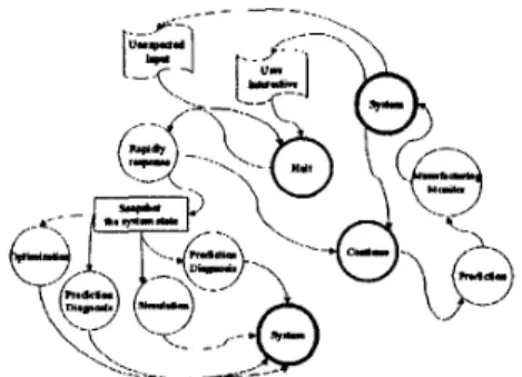
Although we can obtain an optimal solution for our proposed evaluation tool, it is only for a static and

Figure 5: The negotiation network of multi-objective function

Figure 6: General approach for operation deterministic one based on the current information. However, the manufacturing environment changes dy- namically. One simple rescheduling policy is to perform the optimization module periodically. However, when any stochastic event occurs with the period, it is needed to respond to that situation. Thus, a snapshot is used to report all current manufacturing informa- tion, and the Rapidly Response Module will determine what is the better timeslot of this snapshot. The approach of operation can be presented in Fig. 6 , whose

details can be described in the following :

(1) First, the model is at System state. If there is not any unexpected input or interaction from users, the model enters into the Continue state; other- wise, it enters into the Halt state. If the model is at the Halt state, the Rapidly Response Mod-

ule will be performed immediately. It determines what is the better timeslot of the snapshot and

decides which is the next process. Go to step(3). (2) If the model is at the Continue state, the Predic-

tion Module and Manufacturing Monitor Module

will be executed. Go to step(5).

(3) If the model does not have to respond to exterior events, the state of the model is set to the Con-

tinue state. Go to step (2). Otherwise, perform accurate module properly.

(4) If the module is completed, the state of the model is set to the System state. Go to step (1).

(5) The state of the model is set to the System state. Go to step (1).

The objective of a prediction diagnosis is to minimize equation (2). First, the following initializations are made before we proceed to a detailed analysis G f

performance prediction:

(a) Jobs arrive at the manufacturing system randomly and follow a well-known static process. The processing-times for each machine are common random variables, which are well known dis- tributions with certain mean value.

(5)

(b) The jobs scheduling is guided by a planned control policy or schedule R that is being evaluated, and the routing of the jobs through the machines are with a fixed probability.

Let the prediction rule

PO

follows the elementary queuing theory with some tuning variables. With using the result from elementary queuing theory and tech- niques of the Laplace transforms, the waiting time and flow-time will be approximated as Eo(W) and Eo(F), respectively, and the approximated prediction of performance can be calculated accordingly.

The prediction-diagnosis process coordinates with the approach of model operation for each run i, and the algorithm of prediction-diagnosis process can be summarized in the following steps:

(1) Use Prediction rule

P

i

to approximates Ei(W)

and E i ( F ) . The new actual P o s t E i ( W ) and

P o s t E i ( F ) will be calculated, where P o s t E i ( W )

and PostEi ( F ) differ from Ei ( W ) and Ei ( F )

,

by that they are post-predicted data.

(2) Examine Pi subject to equation (2) in this times-

lot of snapshot. Form the new Pi+l with reference to the performance of post-prediction according to equation (2).

3.3 Optimization Conducting Process

The algorithm of optimization conducting process can be summarized in the following steps.

(1) Simulate N inputs using approximated values.

Use the idea of the $-transform and [ method proposed by Chichinadze(l969) subject to mini- mization of the equation (3) and (4), and let R:ck

be the estimation of optimal control policy Rack. (2) If the estimation error is large, then go back to

step (1). Find all of neighbors R:Zk of RGck. Co- ordinate with each run i of prediction diagnosis process, and find the best R:Zk such that the value of Vi**

(Pi)

is the minimum. Replace R;flck with

R:zk. ack

Notice that the step (1) consists of running of local optimization calculating several times, and step (2) is a heuristic method in order to forecast the domain of solutions, and to make use of the data generated by prediction as the direction to find the optimum.

3.4 Multi-objective Negotiation Process

First, we introduce a relational network called nego-

tiation network. The negotiation network is presented

in Fig. 5. Its nodes composed of planned control policy

R being evaluated, characteristic variable(CV), objective of requirement OR and final objective function

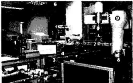
Figure 7: Two-robot assembly cell. 1 : Part loader, 2 :

Parts, 3 : Conveyor belt, 4 : Optical sensors, 5 : CRS robot arm, 6 : Overhead CCD camera, 7 : rotatory buffer, 8 : Grippers of Adept, 9 : Adept robot arm.

in equation (5)and(7). Relatively, its arcs can be la- beled with the elements Mij of relationship matrix

M , the impact function

ai,

and weighting parameters ~ 1 , .

. .

,

(YN. With the negotiation network we proposed, the problem of multi-objective can be trans- lated into a dual problem. It is to balance the flow for each arc in the network. There is a heuristic algorithm for the dual problem that can be summarized in the following steps. Notice that the multi-objective negotiation process coordinates with the approach of model operation per iteration i.

Give an objective f ( R ) . According to the objec-

tive f ( R ) , tune the value of weighting parameters Check each node O R j , examine the input stream and output stream of node ORj, i.e., calculating the ratio of the values

nj

.

If the result is too large, then modify R.

f f l , " ' , f f N .

E.

MzjCVi

Simulation Verification on An Exam-

ple

4.1 Example Description

In this paper, several simulations on an example are performed to verify our proposed evaluation tool. In our laboratory, we have a two-robot assembly cell shown in Fig. 7, that is dedicated to assemble various types of mechanical parts sent serially into the conveyor belt by the part loader. There are two products produced in our assemby cell, and each product has four parts that are assembled by the robot manipula- tor. Parts can be placed randomly in the pallet of the loader. The loader will load the part onto the conveyor belt one at a time on request. Each robot has different mean time between failure (MTBF) and mean time to repair (MTTR). There are three objectives to be

(6)

Table 1: Arrived parts by the end of each hour

achieved, they are cycle-time(CT), throughput(TP) and Working in process(W1P) respectively. The sim- ulation time horizon is 6 hours. At the beginning, there are 16 initial parts in this assembly cell. The

total number of arrived parts at the end of each hour is listed in Table 1. For each case, three simulation runs are performed under the dynamic and stochastic environment, by choosing three different combinations of weighting parameters ai in the objection function

at Equation (7), they are {4,3,3},{2,3,5} and {4,2,4}

respectively

.

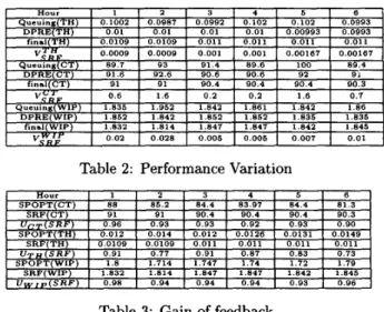
4.2 Simulation Results

This simulation is run on a Pentium PC, and the results that we will examine are the prediction uarza- tion V q ( P t ) in equation (2) and the gain of feedback

U,(R):n equation (3). They are shown in Table 2 and Table 3. For illustration, we only present the result while the combinations of weighting parameters is {4,2,4}. We let the original planned assembly scheduling is a shortest remaining first(SRF) method,

it means that robots assemble the parts or subassembly products when the parts or subassembly products have shortest remaining steps to be a final product.

If we assume the actual arriving time of part in the pallet and the processing time of robot are random numbers with uniform distribution(minimum=0.0093, maximum =0.0135) and expo- nential distribution(mean=30) respectively, then we have the mean value of performance prediction for ap- plying the queuing theorem. However, the runs are performed under the dynamic and stochastic environment, we have the mean value for using the method of diagnosed prediction. F’rom these results, the prediction diagnosis will work properly within the stochastic and state-dependent environment.

The SRF method is good for our assembly cell.

However, we can observe that the simulation and prediction based optimization can improve all the above criteria in the log run, i.e., we have shorter mean value of cycle time, higher mean value of throughput and lower mean value of WIP

.

With optimization based scheduling however, the WIP is stabilized and lower than those corresponding to the heuristic dispatching rules. The results also show that the proposed on-line evaluation tool can work properly.

-

Hoy. 1 - 2 3 4 5 6

Queuin.(TH) 0 I002 0 0987 0 0992 0 102 0 102 0 0993 D P R E ( T H ) 001 0 01 0 01 0 01 000993 0 0993

00009 0 0009 0 001 0001 0 00167 000167

’ fmd(TH) 00109 00109 0011 0011 0011 0011

Table 2: Performance Variation

Hour 1 1 1 2 1 3 1 4 1 5 1 6

S P O P T ( C T ) I 88 I 85.2 I 84.4 I 83.97 I 84.4 I 81.3

a1 I a i I a n a I a n a I a n a I a n 3

Table 3: Gain of feedback

5 Concluding Remarks

This paper proposes a new on-line evaluation tool wherein original planned control policy designed by engineers will be evaluated before issued. A new optimal control rule or schedule derived from the original planned one will be given. We also analyze the multi- objective problem by a negotiation net. The results show the intelligence and efficiency of the proposed on-line evaluation tool.

References

Robert and Alan, “Performance evaluation of automated manufacturing systems using generalized stochastic Petri Nets,” IEEE Transactions o n Robotics and Automation,

Vol. 6, NO. 6, pp. 621-639, DEC 1990.

Samir M. Koriem and L. M. Patnaik, “A generalized stochas- tic high-level Petri Net model for performance analysis,”

Journal of Systems Software, pp. 247-265,36, 1997. T. C. E. Cheng, “Optimal due-date assignment in a job shop,”

Journal of Prod. Res., Vol. 24, No. 3, pp. 503-515, 1986.

Alexandre Dolgui and Dmitry Ofitserov, “A stochastic method for discrete and continuous optimization in manu- facturing systems,” Journal of Intelligent Manufacturing,

pp. 405-413, August 1997.

Jian Yang and Tsu-Shuan Chang, “Multiobjective scheduling for IC sort and test with a simulation tested,” IEEE Trans- actions o n Semiconductor Manufacturing, Vol. 1 1 , No. 2, pp. 304-315, MAY 1998.

Shouju Ren, Xiao Dong Zhang and Xi Ping Zhang, “A new generation of decision support system for advanced manu- facturing enterprises,” Journal of Intellagent Manufacturmg,

pp. 335-343, August 1997.

Paul P.M. Stoop and J . Will M . Bertrand, “Performance pre- diction and diagnosis in two production departments,” Jour-