國立交通大學
應用數學系
數學建模與科學計算碩士班
碩士論文
效率市場假說驗證:
動態調整交易系統之全球股、匯市測試
Verification on market efficiency:
Dynamic Trading Indicators on global Equity and
Currency Markets
研究生:張裕昇
指導教授:賴明治博士 周國端博士
效率市場假說驗證:
動態調整交易系統之全球股、匯市測試
研究生:張裕昇 指導教授:賴明治博士
周國端博士
國立交通大學
應用數學系數學建模與科學計算碩士班
摘要
行為財務學(behavioral finance)與傳統技術分析都有相似的起源, 兩者皆導因 於,假設人類的投資行為其實會受到外來環境影響,而產生傳統財務學者所認為 的『不理性』行為;且兩者皆藉由試圖辨識人類行為的模式,以尋找可能的市場 超額利潤。基於是傳統財務學的代表,效率市場假說(Efficient Market Hypothesis)一直被測試其真實性與可靠性,但其仍然是目前學術界未有肯定答案 的問題。效率市場假說認為,『市場價格已經隱含了所有可取得資訊的影響力』, 其意味著無人能對未來價格形成持續並成功地預測;另一方面,像技術分析這類 的交易指標,其正是透過對過去價格走勢與市場型態的研究,試圖尋找未來可能 的類似走勢,以期達到擊敗市場的目標。基於交易策略的超額報酬能視為預測能 力的展現,交易指標應能當作效率市場假說的驗證方法。本論文透過創立一個『自 動交易流程』,其包含『動態調整交易指標』與統計方法『決策樹(Classificationand Regression Tree)』,以驗證目前全球股、匯市之超額報酬取得的可能性。本
篇論文的結論是,我們所提供的方法的確在新興市場的股、匯市獲取極高之樣本 外超額報酬,然而在已開發國家之股、匯市則無明顯擊敗市場報酬之能力;導致我 們無法於,以開發國家獲取超額報酬的原因,可能可指向金融市場的反射理論 (reflexivity)。
關鍵字: 行為財務學, 效率市場假說, 動態調整交易指標,
Verification on market efficiency:
Dynamic Trading Indicators on global
Equity and Currency Markets
Student: Yu-Sheng Chang Advisor: Dr. Ming-Chih Lai
Dr. David Jou
Department of Applied Mathematics
Institute of Mathematical Modeling and Scientific Computing
National Chiao Tung University
Abstract
Behavioral finance and traditional technical trading indicators are similar in their roots. Both are rooted in the assumption that man acts for behavioral reasons in ways that may seem irrational by the standards of classical finance. Both of them approach financial markets by identifying patterns of human behavior to uncover opportunities of profits. On the behalf of classical finance, “Efficient Market Hypothesis” (EMH) has been testing for its validity, though it’s still an unsolved argument for academic finance now. The EMH states that the current market price incorporates all the information available, which leads to a conclusion that given the information available, no prediction of the future price changes can be made. On the other hand, trading indicator such as technical analysis, which is essentially the search for recurrent and predictable patterns in asset prices, attempts to forecast future price changes. To the extend that return of a trading strategy can be regarded as a measure of predictability, trading indicator can be seen as a test of the EMH. This paper attempts on creating an automated trading process, which includes “dynamic technical trading indicators” and statistical method “CART” (Classification and Regression Tree) to check the
profitability on global equity and Currency Markets. We conclude that, our testing methods do make obvious positive profits on developing countries’ equity and foreign currency markets; the reason why our method can’t generate obvious positive profit in developed countries maybe can point to the “reflexivity” of financial market.
Keywords: behavioral finance, efficient market hypothesis, dynamic trading indicator, CART, reflexivity
誌 謝
光 陰 似 箭 , 日 月 如 梭 , 很 快 地 這 兩 年 的 碩 士 生 涯 就 這 們 悄 悄 地 結 束 了; 對 我 而 言 … 這 不 是 個 終 點, 而 是 下 一 個 挑 戰 的 起 跑 點。 首 先,要 謝 謝 我 的 指 導 教 授 賴 明 治 老 師 、 周 國 端 老 師 和 我 在 宏 泰 人 壽 的 主 管 吳 志 遠 博 士,感 謝 您 們 讓 我 在 碩 士 生 涯 中,能 盡 情 地 發 揮 所 長 並 提 早 進 入 法 人 金 融 市 場,從 而 讓 我 可 以 寫 出 一 篇 結 合 數 學 與 實 務 的 財 務 論 文;有 了 您 三 位 老 師 的 指 導 與 協 助,讓 我 能 在 這 兩 年 當 中,更 持 續 地 在 金 融 實 務 與 應 用 數 學 中,有 了 更 深 一 層 的 瞭 解 與 結 合,相 信 這 都 將 成 為 未 來 我 持 續 自 我 超 越 的 關 鍵 因 素。此 外,在 論 文 審 核 期 間,承 蒙 鉅 融 資 本 管 理 的 鄭 振 和 博 士 費 心 審 閱 並 提 供 許 多 寶 貴 意 見,讓 我 可 以 在 財 務 數 學 這 一 塊,有 很 大 的 觀 念 性 突 破 , 老 師 這 一 切 的 指 導 , 學 生 將 永 銘 在 心 。 感 謝 我 的 同 窗 好 友 仁 洲 與 振 庭 , 謝 謝 你 們 在 程 式 撰 寫 與 數 學 模 型 方 面,給 了 我 很 大 的 協 助 與 討 論,我 不 會 忘 記 你 們 的 ! 往 後 的 日 子,希 望 我 們 能 持 續 地 往 我 們 的 夢 想 邁 進 , 有 朝 一 日 一 定 要 有 我 們 自 己 的 事 業 與 成 就 ! 此 外,亦 很 感 謝 彥 琳,謝 謝 妳 在 我 論 文 後 期 與 口 試 中,所 做 的 許 多 貼 心 幫 忙 , 還 有 清 和 學 長 、 哲 維 、 昆 霖 、 建 興 、 昱 丞 、 小 李 與 其 他 建 模 所 、 應 數 所 的 同 窗 們,除 了 在 課 業 上 的 互 相 切 磋,閒 暇 之 餘 還 能 與 你 們 閒 話 家 常 , 讓 我 生 活 充 滿 樂 趣 , 謝 謝 你 們 … 希 望 我 們 第 一 屆 的 建 模 所 同 窗 畢 業 後, 大 家 以 後 都 能 有 很 好 的 發 展,一 定 要 把『 建 模 所 』這 塊 招 牌 給 擦 亮 ! 接 下 來 要 謝 謝 我 在 宏 泰 人 壽 認 識 的 朋 友 們 仲 苑 、 雨 賢 、 于 揚 、 靜 玟 、 益 宗 、 柏 君 、 家 堯 、 孟 翰 、 伯 瑋 與 其 他 財 工 部 、 固 收 部 、 經 濟 研 究 室 的 長 官 與 同 事 們,感 謝 這 段 時 間 你 們 對 我 的 幫 忙 與 照 顧,讓 我 可 以 在 這 邊 愉 悅 地 工 作 與 成 長 , 祝 福 大 家 以 後 能 工 作 順 心 、 步 步 高 升 。 最 後,也 最 重 要 的,我 要 感 謝 我 的 爸 爸、媽 媽 與 姊 姊、哥 哥,謝 謝 爸 、 媽 從 小 辛 苦 地 養 育 我 成 人 , 讓 我 誠 摯 地 說 :『 謝 謝 您 , 辛 苦 了 ! 』, 沒 有 家 人 的 關 心 與 祝 福,我 無 法 順 利 的 完 成 學 業,願 與 他 們 以 及 所 有 在 我 周 圍 關 心 我 的 人 , 一 同 分 享 此 篇 論 文 完 成 之 喜 悅 與 榮 耀 。張裕昇 2009/9/10
Content
Contents……….Ⅰ I. List of tables………..Ⅱ II. List of figures………....Ⅲ
1. Introduction………..1
2. Theory and Literature Review………...3
2.1 Technical Trading Indicators………...3
2.2 CART(Classification and Regression Tree)………6
2.3 Representative Studies………...8
3. Methodology and Empirical results……….11
3.1 Currency Market………12
3.1.1 Single Moving Average……….12
3.1.2 Dual Moving Average………13
3.1.3 Combination of Single Moving average with stochastic oscillator…..15
3.2 Equity Market……….19
3.2.1 Single Moving Average……….19
3.2.2 Dual Moving Average………21
3.2.3 Combination of Single Moving average with stochastic oscillator…..22
3.3 Discussion on the appropriateness of our trading criteria………..24
3.3.1 The trade off between stabilization and efficiency………24
3.3.2 The choice of back-test and forecasting Period………....27
3.4 The issue of reflexivity………..27
3.4.1 CART analysis on stochastic oscillator………..29
3.4.2 The selection of price in entering and exiting position ………32
4. Conclusion………..35
Reference………37
List of Tables
Table 1: The equity and currency we will research on Global-Twenty………11
Table 2: The result sheet of s=1, l:20~240 under MA System……….12
Table 3: The result sheet of s:2~10, l:20~240 under MA System………13
Table 4: The result sheet of MK model in currency market……….16
Table 5: The beta sheet of MK model in currency market………...17
Table 6: The P-value sheet of MK strategy with buy&hold……….18
Table 7: The result sheet of s=1, l:20~240 under MA System……….19
Table 8: The beta sheet of single MA strategy in equity market………..20
Table 9: The P-value sheet of single MA with buy&hold………20
Table 10: The result sheet of s: 2~10, l: 20~240 under MA System………21
Table 11: The result sheet of MK model in equity market………...22
Table 12: The beta sheet of MK model in equity market……….23
Table 13: The P-value sheet of MK strategy with buy&hold………...23
Table 14: MK model for currency under different training period………...27
Table 15: MK model for equity under different training period………...27
Table 16: The return sheet of CART on KD(9,3,3)………..31
Table 17: The comparison sheet of different used price in single MA on currency……….32
Table 18: The comparison sheet of different used price in MK model on currency………33
Table 19: The comparison sheet of different used price in single MA on equity………….33
List of Figures
Figure 1: Binary tree separation in CART……….7
Figure.2: TWD performance under S=1, L: 20~240 of MA strategy………...14
Figure.3: TWD performance under S:2~10, L: 20~240 of MA strategy………..14
Figure.4: AUD performance under Single Moving Average strategy………..16
Figure.5: AUD performance under MK model strategy………...17
Figure.6: TWD performance under MK model with consecutive set=2………..24
Figure.7: TWD performance under MK model with consecutive set=5………..24
Figure.8: RUB performance under MK model with consecutive set=2...25
Figure.9: RUB performance under MK model with consecutive set=5………...25
Figure.10: TWOTC_Index performance under MK model with no consecutive set... 26
Figure.11: TWOTC_Index performance under MK model consecutive set=2...26
Figure.12: KD(9,3,3) on S&P 500 in 1953~2008……….29
Figure.13: Classification table by CART on INDU in 2007………30
Figure.14: The chart of currency portfolio in MK with DXY………..36
1. Introduction
With the rapid openness and change of Taiwan’s financial market, it’s
becoming more and more important for Taiwan’s institutional investors to be able to develop a global financial market monitoring system. The reason why we need not only the globalization of this world but also due to Taiwan financial supervisor deciding to permit opening up running of hedge fund in this island in the near term. If we just don’t want this shares being taken again by foreign investment banking, it’s really important now for Taiwan’s financial community to strike out a global financial market trading system to compete with foreign investment banking. Seeing the responsibility I should take, I decided to check carefully on EMH with global equity and currency markets. See if we can do something or at least knowing that maybe what financial institution’s Advertisement on TV need we think again rather than invest in their fund with fantasy.
Where I start from is technical analysis. Technical analysis is a forecasting method of price movements using past prices, volume, and open interest. Pring (1991), a leading technical analyst, provides a more specific definition: “The technical approach to investment is essentially a reflection of the idea that prices move in trends which are determined by the changing attitudes of investors toward a variety of economic, monetary, political and psychological forces... Since the technical approach is based on the theory that the price is a reflection of mass psychology ("the crowd") in action, it attempts to forecast future price movements on the assumption that crowd psychology moves between panic, fear, and
pessimism on one hand and confidence, excessive optimism, and greed on the other.”
Technical analysis includes a variety of forecasting techniques such as chart analysis, cycle analysis, and computerized technical trading systems. A technical trading system consists of a set of trading rules that result from parameterizations, and each trading rule generates trading signals (long, short, or out of market) according to their parameter values. Several popular technical trading Indicators are moving averages, channels, and momentum oscillators. Since Charles H. Dow first introduced the “Dow theory” in the late 1800s, technical analysis has been extensively used among market participants such as brokers, dealers, fund
managers, speculators, and individual investors in the financial industry. Numerous surveys indicate that practitioners attribute a significant role to technical analysis. For example, futures fund managers rely heavily on computer-guided technical trading systems (Irwin and Brorsen 1985; Billingsley and Chance 1996), and about 30% to 40% of foreign currency traders around the world believe that technical
analysis is the major factor determining exchange rates in the short-run up to six months (e.g., Menkhoff 1997; Cheung and Wong 2000; Cheung and Chinn 2001). Despite its long history, technical analysis and its claims have traditionally been regarded by academics with a mixture of suspicion and contempt. However, a renewal of academic interesting in such forecasting techniques has been sparked by accumulating evidence that financial markets may be less efficient than was originally believed. Foreign exchange markets have proved to be more volatile than it was anticipated at the beginning of the floating rate era in the early 1970s, and the "long swings" in the dollar observed in the 1980s have not been satisfactorily
explained in terms of movements in economic fundamentals. Several studies have sought to document the existence of excess returns to various types of trading rules in the foreign exchange market (Dooley and Shafer (1983), Levich and Thomas (1993), Osler and Chang (1995)). These papers find that a class of trading rules makes economically significant excess returns in a variety of currencies over different time periods; however, these results are difficult to interpret. Because the rules considered in these studies are selected for examination, there is an
inevitable risk of bias. For example, if someone uses 60-days moving average as a trading indicator and claims that he can get positive risk-adjusted return by this way, I think it may cast many subsequent problems such as “why we use parameter of 60-day?” or “Why we can claim that the successful using parameter in the sample we test can continuously usable on follow-up days that is out of our testing
sample?”
In this paper, we address this problem by using a dynamic parameter-adjusting method as a search procedure for identifying optimal trading rules. We obtain rules from a sample period then we use the sample-training parameter on the
out-of-sample period and recursively run this procedure from 2000 to 2008 for global-twenty economically important countries’ equity and currency market. The advantage of this approach, and the most important contribution of the paper, is that it enables us to construct a true out-of-sample test of the significance of the excess returns earned by the trading rules. We find strong evidence of significant excess risk-adjusted returns after transaction costs both on equity and currency market, but it does perform better on developing market. To ensure on the possible observed excess returns, we calculate beta for the returns from our portfolio with benchmark indices, and implement the statistical significance test. Then we find that no
evidence of significant systematic risk associated with use of our trading strategy and most of the assets we observe almost have higher mean of return than buy&hold strategy.
watched technical Indicators such as KD(9,3,3) to see if we can advantage on the phenomena of widely using technical analysis on financial market. The
performance of returns shows the strategy can beat original KD(9,3,3) by far, but in some market, this KD method characterized by CART may not be appropriate.
The paper is organized as follows. Section II reviews the previous work of technical analysis on financial market. Section III discusses the implementation of our dynamic trading indicator and shows the results on global equity and currency markets. Section IV presents the results and draws conclusions.
2. Theory and Literature Review
Before reviewing historical research, it is useful to first introduce and explicitly define major types of technical trading indicators and the statistical method CART that we use in classification technical indicators.
2.1 Technical Trading Indicators
A technical trading system comprises a set of trading rules that can be used to generate trading signals. In general, a simple trading system has one or two
parameters that determine the timing of trading signals. Each rule contained in a trading system is the results of parameterizations. For example, the Dual Moving Average Crossover system with two parameters (a short moving average and a long moving average) may be composed of hundreds of trading rules that can be generated by altering combinations of the two parameters. Among technical trading systems, the most well-known types of systems are moving averages, channels (support and resistance), momentum oscillators, and filters. These systems have been widely used by academics, market participants or both, and, with the
exception of filter rules, have been prominently featured in well-known books on technical analysis, such as Schwager (1996), Kaufman (1998), and Pring (2002). Filter rules were exhaustively tested by academics for several decades (the early 1960s through the early 1990s) before moving average systems gained popularity in academic research. This section describes representative trading systems for each major category: Dual Moving Average Crossover, Outside Price Channel (Support and Resistance), Stochastic Oscillator and Alexander’s Filter Rule.
Dual Moving Average Crossover
Moving average based trading systems are the simplest and most popular trend-following systems among practitioners (Taylor and Allen 1992; Lui and Mole 1998). According to Neftci (1991), the (dual) moving average method is one of the
few technical trading procedures that is statistically well defined. The Dual Moving Average Crossover system generates trading signals by identifying when the short-term trend rises above or below the long-term trend.
Specifications of the system are as follows: A. Definitions
1. Shorter Moving Average over s days at time t (SMAt)=
∑
= −+ s i c i t s P 1 1/
Where c is the close price at time t and s<t
t
P
2. Longer Moving Average over l days at time t (LMAt)=
∑
= −+ l i c i t l P 1 1/ Where s<l ≤t B. Trading rules 1. Go long at c if > t P (SMAt) (LMAt) 2. Go short at c if < t P (SMAt) (LMAt) C. Parameters: s, l.
Outside Price Channel
Next to moving averages, price channels are also extensively used in technical trading methods. The fundamental characteristic underlying price channel system is that market movement to a new high or low suggests a continued trend in the direction established. Thus, all price channels generate trading signals based on a comparison between today’s price level with price levels of some specified number of days in the past. The Outside Price Channel system is analogous to a trading system introduced by Donchian (1960), who used only two preceding calendar week’s ranges as a channel length. More specifically, this system generates a buy signal when the close price is outside (greater than) the highest price in a channel length (specified time interval) and vice versa.
Specifications of the system are as follows: A. Definitions
1. Price channel = a time interval including today, n days in length.
2. The Highest High = , where is the high price
at time t-1. ) (HHt max{ 1,..., thn 1} h t P P− − + h t P−1
2. The Lowest Low (LLt)=min{ 1,..., tln 1}, where is the low price at
l t P
P− − + l t
time t-1. B. Trading rules
1. Go long at c if > , where is the close price at time t.
t P c t P (HHt) Ptc 2. Go short at c if < . t P c t P (LLt) C. Parameter: n. Stochastic oscillator
The stochastic oscillator(SO) is a momentum indicator used in technical analysis, introduced by George Lane (1956) to compare the close price of a
commodity to its price series over a given time span. The idea behind this indicator is that price tends to close near their past highs in bull markets, and near their lows in bear markets. Generally, trading signals can be spotted when the stochastic oscillator crosses its moving average. Two stochastic oscillator indicators are typically calculated to assess future variations in prices: fast (denoted by K) and slow (D). Comparisons of these statistics are a good indicator of speed at which prices are changing or the Impulse of Price. Some analysts argue that K or D levels above 70 and below 30 can be interpreted as overbought or oversold. On the theory of price oscillating, George Lane, recommend that buying and selling be timed to the return from these thresholds. In other words, one should buy or sell after a bit of a reversal. Practically, this means that once the price exceeds one of these
thresholds, the investor should wait for prices to return through those thresholds (e.g. if the oscillator were to go above 80, the investor waits until it falls below 80 to sell)
Specifications of the system are as follows: A. Definitions
1. Stochastic oscillator Value(SOVt) = [ c- ] / [ - ]
t
P (LLt) (HHt) (LLt)
c t
P , (LLt), (HHt) are the same definitions in Outside Price Channel.
2. = = , i.e. K is the s-days moving
average of SOV, and D is the l-days moving average of K
t K
∑
= −+ s i t i s SOV 1 1/ Dt∑
= −+ l i t i l K 1 1/ B. Trading rules 1. Go long at c if ( < ) → ( > ) unless (K<25) t P Kt−1 Dt−1 Kt Dt 2. Go short at c if ( > ) → ( < ) unless (K>75) t P Kt−1 Dt−1 Kt DtC. Parameter: n, s, l
There are two items about Stochastic Oscillator to explain here. First, the parameter are default generally set as (9,3,3) in worldwide financial website, such as Bloomberg, MarketWatch, yahoo finance and CnYes. In the “Reflexivity” section, we will deeply discuss the commonly used parameter in the SO indicator. Second, the reason why we add a rule on holding our position of threshold value 25 and 75 is that when K value keeps going above 75 as price series moving forward means the price series are in a strong bullish trend or better than 3rd-Quartile in statistical way. Since that reason, we should not unwind our long position as the K value higher than 75 and vice versa.
.Alexander’s Filter Rule
This system was first introduced by Alexander (1961, 1964) and exhaustively tested by numerous academics until the early 1990s. Since then, its popularity among academics has been replaced by moving average methods. This system generates a buy (sell) signal when today’s closing price rises (falls) by x% above (below) its most recent low (high). Moves less than x% in either direction are
ignored. Thus, all price movements smaller than a specified size are filtered out and the remaining movements are examined. Alexander (1961, p. 23) argued that “If stock price movements were generated by a trendless random walk, these filters could be expected to yield zero profits, or to vary from zero profits, both positively and negatively, in a random manner.”
Specifications of the system are as follows: A. Definitions and abbreviations
1. High Extreme Point (HEP) = the highest close obtained while in a long trade. 2. Low Extreme Point (LEP) = the lowest close obtained while in a short trade. 3. x = the percent filter size.
B. Trading rules
1. Go long on the close price, if today’s close rises x% above the LEP. 2. Go short on the close price, if today’s close falls x% below the HEP. C. Parameter: x.
2.2 CART(Classification and Regression Tree)
Classification and regression trees (CART) addressed by Breiman is a
non-parametric technique that recursively partitions groups into smaller subgroups that maximally differ on a desired outcome. CART produces either classification or regression trees, depending on whether the dependent variable is categorical or numeric, respectively. Trees are formed by a collection of rules based on values of
certain variables in the modeling data set. Rules are selected based on how well splits based on variables’ values can differentiate observations based on the dependent variable. Once a rule is selected and splits a node into two, the same logic is applied to each “child” node (i.e. it is a recursive procedure) Splitting stops when CART detects no further gain can be made, or some pre-set stopping rules are met.
Each branch of the tree ends in a terminal node which is uniquely and independently defined by a set of rules, and each observation falls into one and exactly one terminal node.
The step of tree growing is as follows:
1. The first step involves calculating Gini impurity function for the parent node, which is sometimes referred to as the Gini diversity index and can be defined as follows: Diversity Index( i(t)) = Φ(p( 1|t ),p( 2|t ),……,p( J|t )) = −
∑
2/
1 pi j
2. The second step involves calculating the Gini diversity index for each of the two child nodes into which the parent node splits.
3. The third step involves calculating the weighted average, according to the proportion of the parent node that is included in each child node, of the Gini diversity indexes for each of the child nodes. This can be obtained by solving the following equation:
Weighted diversity index= [(p1)(diversity index1)]+ [(p2) (diversity index2)],
where p1 and p2 refer to the proportions of the parent node that are included in the respective child nodes.
4. The last step requires calculating the Gini improvement measure, which is equal to the following:
Gini improvement measure = diversity index of parent node - weighted diversity index
The procedure of CART:
‧ Start with all subjects in 1 group (parent node)
‧ Divide parent node into two “child nodes" based on best predictor ‧ Best predictor=lowest impurity ‧ Based on all possible variable splits ‧ Repeat process for each child node Figure 1: Binary tree separation in CART
2.3 Representative Studies
Van Horne &Parker (1967) in their study tested 30 NYSE stocks by daily frequency with period from 1960 to 1966. They use Moving average (100, 150, and 200 days with 0, 2, 5, 10, and 15% as bands to make trading decision) with
transaction costs considered as members of the NYSE’s average. They concluded that “no trading rule earned a total closing balance nearly as large as return
generated under the buy&hold strategy even without considering transaction costs.” Dryden (1970) in his study tested U.K. stock index by daily frequency with period from 1960 to 1967. He use filter rules(12 rules from 0.1% to 5%) with transaction costs considered as 0.625%. He concluded that “Without transaction costs, filter rules consistently beat the B&H strategy. With transaction costs, the returns from the best filter rules were similar to those from the B&H, but long transactions beat the B&H.”
Logue, Sweeney & Willett (1978) in their study tested 7 foreign exchange rates by daily frequency with period from 1973 to 1976. They use filter rules(11 rules from 0.1% to 15%) without considering transaction costs. They concluded that “For every exchange rate (the Mark, Pound, Yen, Lira, France franc, Swiss franc, and Dutch guilder) profits from the best filter rules exceeded those from the B&H strategy by differences ranging from 9.3% to 32.9%.”
Dale & Workman (1980) in their study tested 90-days T-bill future derivative by daily frequency with period from 1976 to 1978. They use Moving average(11 rules from 5 to 60 days ) with transaction costs considered as $60 per roundtrip. They concluded that “For each individual contract, the best trading rules generated positive net returns, although the rules did not indicate consistent performances over the sample period.”
Neftci & Policano (1984) in their study tested 4 futures: Copper, Gold,
Soybeans, and T-bills by daily frequency with period from 1975 to 1980. They use Moving average (25, 50, and 100 days) without considering transaction costs. They concluded that “Not adjusted Trading signals were incorporated as a dummy
variable into a regression equation for the minimum mean square error prediction. Then the significance of the dummy variable was evaluated by F-test. Overall, Moving average rules indicated some predictive power for T-bills, gold, and soybeans.”
Brock, Lakonishok & LeBaron (1992) in their study tested Dow Jones Industrial Average by daily frequency with period from 1897 to 1986. They use Moving
average(1/50, 1/150, 5/150, 1/200, and 2/200 days with 0 and 1% bands ) without considering transaction costs. They concluded that “Before transaction costs, buy (sell) positions across all trading rules consistently generated higher (lower) mean
returns than unconditional mean returns, and these results were highly significant in most cases. For example, a mean buy return from variable moving average rules was about 12% per year and a mean sell return was about -7%. Moreover, the buy returns were even less volatile than the sell returns. Simulated series from a
random walk with a drift, AR (1), GARCH-M, and EGARCH models using a
bootstrap method could not explain returns and volatility of the actual Dow series” Farrell & Olszewski (1993) in their study testedS&P 500 futures by daily frequency with period from 1982 to 1990. They use a nonlinear trading strategy based on ARMA (1,1) model with transaction cost considered as 0.0025%. They concluded that “Although the nonlinear trading strategy were slightly more profitable than the B&H strategy, the result was statistically insignificant.”
Ratner & Leal (1999) in their study tested 10 equity indices in Asia and Latin America by daily frequency with period from 1982 to 1995. They use Moving average(1/50, 1/150, 5/150, 1/200, and 2/200 days with bands of zero and one standard deviation) with transaction costs considered between 0.5%~2%. They concluded that “After transaction costs deducted, 21 out of 100 trading rules that were applied to the 10 indices generating statistically significant returns (18.2% to 32.1% per year) with the profitability concentrated in four markets: Mexico, Taiwan, Thailand, and the Philippines.When statistical significance was ignored, 82 out of the 100 rules appeared to have forecasting ability in emerging markets.”
Goodacre & Kohn-Sprever (2001) in their study tested a random sample of 322 companies from the S&P 500 by daily frequency. They use its own creating system named CRISMA (combination system of Cumulative volume, RelatIve Strength, and Moving Average) to observe prior 200 days’ best performing parameter to apply on next out-of-sample period from 1988 to 1996 with transaction costs considered between 0%~2% . They concluded that “The CRISMA system generated annualized profits ranging 6.2% to 17.6% depending on transaction costs, while the annualized return on the S&P 500 Index over the same time period was 14.2%.”
Lee, Gleason & Mathur (2001) in their study tested 13 Latin American currencies by daily frequency with period from 1992 to 1999. They use Moving average(short moving average:1~9 days, long moving average:10~30 days and channels:2~50 days) with transaction costs considered as 0.1%. They concluded that “Out-of-sample results showed that moving average rules generated
significantly positive returns for currencies of four countries: Brazil, Mexico, Peru, and Venezuela. Channel rules also produced significant profits for the same currencies except that of Peru. When only long positions were considered, there was a marginal improvement to five and four currencies for moving average rules
and channel rules, respectively.”
Olson (2004) in his study tested 18 exchange rates by daily frequency. He used moving average (short moving average: 1~12 days, long moving average: 5~200 days) to observe past 5 years best performing parameter to apply on next out-of-sample 5 years from 1976~2000 with transaction costs considered as 0.1%. He concluded that “Out-of-sample results indicated that risk-adjusted trading profits for individual currencies and an equal-weighted 18-currency portfolio declined over time. For the 18-currency portfolio, annualized risk-adjusted returns decreased from an average of over 3% in the late 1970s and early 1980s to about zero percent in the late 1990s. Overall, profits of moving average rules in foreign exchange markets have declined over time.”
From the studies above, I think maybe there are some point can be revised, improved, and kept on
1. To avoid “Selection Bias” problem (Jensen, 1970), we do need to test data by “in-sample and out-of-sample recursive principle” to ensure the claim of profitability of our testing methods.
2. To avert “Data Snooping” problem (White,2000), it had better we test as more indices in equity and currency market as possible.
3. Although sometimes it’s unavoidable, the system we design should be as less component of experience as possible, so I think the parameter inputs shouldn’t be only a few to choose, it may be more appropriate to give them as a range. 4. Due to most of the data researched are before 2000, It may be interesting to
check the methods addressed by Olson(2004) to see if the data outcome can have another explanation in 2001~2008.
5. In the previous study, the trading rules almost concentrated on Filters, Moving average, Price channel; however, the “Stochastic oscillator” is still another worldwide using technical indicator. It may be able to find something in this technical indicator.
3. Methodology and Empirical results
Before we start introducing our trading system, there are some prerequisites and assumptions to announce.
① Experimental object : Global-Twenty economically important countries’ equity and currency market (Table 1)
② Experimental Period : 2000 trading days which is about 2001~2008
③ Back testing and forecasting method : Calculate prior 60-trading days’ best performance parameter and apply it on next 60-days recursively ④ Transaction costs: Equity market is 0.25%, Currency market is 0.15%, and
all of the transactions below have deducted transaction costs in return unless we identify it specifically .
⑤ Parameter range given:
Ⅰ. Moving Average system:
s
is set between 1~10, andl
is set between 20~240 Ⅱ. Stochastic oscillator system:n
is set between 10~20,s
is set between 3~10, andl
is set between 3~10⑥ The price of Entering and unwinding position: Close price of the asset
Stock Currency Stock Currency
Australian
AS51_Index AUDBrazil
IBOV_Index BRLCanada
SPTSX_Index CADIndonesia
JCI_Index IDRSwitzerland
CHFIndia
SENSEX_Index INRCCMP_Index
Korea
KOSPI_Index KRWU.S.
SPX_Index DXY
Mexico
MEXBOL_Index MXNCAC_Index
Philippines
PCOMP_Index PHPDAX_Index
Russia
RUBEurope
SX5E_Index
EUR
Singapore
STI_Index SGDU.K.
UKX_Index GBPThailand
SET_Index THBNKY_Index TWSE_Index
Japan
TPX_Index JPY
Taiwan
TWOTCI_Equity TWDNew Zealand
NZDSouth Africa
ZARHong Kong
HSI_IndexMalaysia
KLCI_IndexChina
SHCOMP_Index Table 1: The equity and currency we will research on Global-Twenty.3.1 Currency Market
3.1.1 Single Moving Average
In this part we test the situation of SMA=1, meaning that we choose the close price series as the parameter of SMA, and the parameters of LMA is set as
previous described “20~240”. In each 60-trading days, we use best performing parameter of the prior 60-trading days which includes 221 kinds of method in characterizing this financial market.
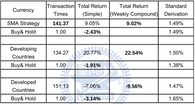
Currency Transaction Times Total Return (Simple) Total Return (Weekly Compound) Standard Derivation SMA Strategy 141.37 9.05% 9.02% 1.49% Buy& Hold 1.00 -2.43% 1.49% Developing Countries 134.27 20.77% 22.54% 1.50% Buy& Hold 1.00 -1.91% 1.38% Developed Countries 151.13 -7.06% -9.56% 1.47% Buy& Hold 1.00 -3.14% 1.65%
Table 2: The result sheet of s=1, l:20~240 under MA System(Summary)
The table above is the summary report of the trading strategy, and we put a detailed form with each currency disclosed in appendix. The portfolio return means the equally-weighted return of these currencies, and we observe that the portfolio’ total return of Dynamic MA “9.02%” is just a little higher than buy&hold one. Besides, we can observe obviously that the portfolio return of developing countries is higher than developed ones; this will be the common situation we see in the upcoming introduced strategies, and we shall discuss the phenomenon thereafter. Briefly, the critical problem of this method is the transaction times are too frequent. So let’s see if the SMA is replaced by MA(2~10) can we have a result that has less noisy trade.
3.1.2 Dual Moving Average
In this part, we replace SMA from 1 to 2~10, and the method is quite alike
Olson addressing in 2004 but with different experimental and training period. In each 60-trading days, we use best performing parameter of the prior 60-trading days which includes 1,989 kinds of method in characterizing this financial market.
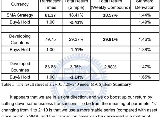
Currency Transaction Times Total Return (Simple) Total Return (Weekly Compound) Standard Derivation SMA Strategy 81.37 18.41% 18.57% 1.44% Buy& Hold 1.00 -2.43% 1.49% Developing Countries 79.75 29.37% 29.91% 1.46% Buy& Hold 1.00 -1.91% 1.38% Developed Countries 83.88 3.35% 2.98% 1.47% Buy& Hold 1.00 -3.14% 1.65%
Table 3: The result sheet of s:2~10, l:20~240 under MA System(Summary)
It appears that we are in a right direction, and we do boost up our return by cutting down some useless transactions. To be true, the meaning of parameter “s” changing from 1 to 2~10 is that we use a more stable series (compared with asset close price) in SMA, and the transaction times can be decreased is a matter of course; however, we may lost some good timing in entering or exiting our position. In establishing trading rules, sometimes we just need to make a trade off between transaction times and stability unless we can find another not fully dependent indicator to help us filter out some more true noise trades. Then, though the trading strategy can beat Buy&Hold strategy, it looks like it isn’t worth taking the risk for the profit we get in this sheet. So we have to refine this strategy further.
In the following graphs (Figure 2, 3), we take TWD as a example of ascending total returns by reducing ineffectual transactions.
Figure.2: TWD performance under S=1, L: 20~240 of MA strategy
Figure.3: TWD performance under S:2~10, L: 20~240 of MA strategy. Compared with figure 2, the transaction times decrease and the total return lift by cutting noisy trades.
3.1.3 Combination of Single Moving average with Stochastic oscillator(MK)
As the description of stochastic oscillator(SO), “Comparisons of these statistics
is a good indicator of speed when prices are changing or the Impulse of Price”; that means stochastic oscillator may help us find good timing of entering or unwinding positions. Before we keep on, we have to clarify the advantages and shortages of MA. “Moving Average” is a trend-follow trading indicator, and the advantage of this indicator is that it will assure you wouldn’t make a wrong position when asset price fluctuates vigorously (rocketing or plunging); however, when asset price series has no clear direction, the MA trading indicator will make many noisy trades which increases unnecessary transaction costs and decreases our return, So it may be meaningful if we combine moving average with stochastic oscillator to see if SO can
help MA find better entry or exit of our position and filter out some noisy trades. The combining logic is as follows:
① Parameter set: 『s:1, l:20~240 under MA System』and 『n:10~20, s:3~10,
l:3~10 under SO System』
② Go long at if ( > LMA) and ( < → > ) unless (K<25) for
two consecutive trading days.
c t
P c t
P Kt−1 Dt−1 Kt Dt
③ Go Short at if ( < LMA) and ( > → < ) unless (K>75) for
two consecutive trading days.
c t
P c t
P Kt−1 Dt−1 Kt Dt
④ In any other situation, we just keep our position.
In each 60-trading days, we use best performing parameter of the prior 60-trading days which includes 155,584 kinds of method in characterizing this financial market.
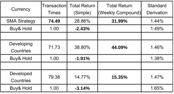
Currency Transaction Times Total Return (Simple) Total Return (Weekly Compound) Standard Derivation SMA Strategy 74.49 28.86% 31.99% 1.44% Buy& Hold 1.00 -2.43% 1.49% Developing Countries 71.73 38.80% 44.09% 1.46% Buy& Hold 1.00 -1.91% 1.38% Developed Countries 79.38 14.77% 15.35% 1.47% Buy& Hold 1.00 -3.14% 1.65%
Table 4:The result sheet of MK model in currency market (Summary)
It seems that we do make some improvements on return of this currency portfolio, it can beat buy&hold strategy by an annualized rate of 3.29% which is
Olson pointed that the moving average rule’ risk-adjusted annualized profit in 1970s. We show an example chart of the difference between Single Moving Average and MK model.
Figure.5: AUD performance under MK model strategy. Comparing Figure 4 and 5, we can easily observe that MK model does filter out some real noisy trades and get a better
entering timing of position.
Then we do some statistics to interpret the connection between our trading strategy and the benchmark index. First, we calculate the beta between each currency trading strategy in MK with Dollar Index daily movement behavior.
Beta coefficient with daily movement of DXY
AUD
-0.06
KRW0.06
BRL0.10
MXN-0.06
CAD-0.04
NZD0.01
CHF-0.07
PHP0.01
DXY-0.10
RUB0.00
EUR0.00
SGD0.00
GBP-0.01
THB-0.02
IDR-0.01
TWD0.02
INR0.02
ZAR-0.11
JPY
-0.02 Currency
Portfolio -0.01
Table 5: The beta sheet of MK model in currency market. Beta value of “ZAR” with “DXY Index”(which is highest in scale) is -0.11, merely equal to zero, which means that our trading strategy has low linear correlation with the benchmark index.
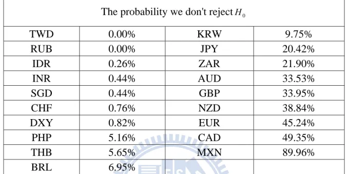
Second, we do the “Tests of Significance” by Z-Test. We want to understand if our trading strategies do have higher mean than original buy&hold ones.
Hypotheses for our test is as follows:
{H0 :μ =μ0, H1:μ >μ0}, μ0 is the mean of asset daily movement return.
The probability we don't reject
H0TWD 0.00% KRW 9.75%
RUB 0.00% JPY 20.42%
IDR 0.26% ZAR 21.90%
INR 0.44% AUD 33.53%
SGD 0.44% GBP 33.95%
CHF 0.76% NZD 38.84%
DXY 0.82% EUR 45.24%
PHP 5.16% CAD 49.35%
THB 5.65% MXN 89.96%
BRL 6.95%
Table 6: The P-value sheet of MK model with buy&hold, which states that our trading strategy’ mean of return is usually higher than buy&hold one except for MXN in terms of Z-test.
3.2 Equity Market
3.2.1 Single Moving Average
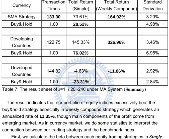
In this part, we test the same situation as in currency market of SMA=1, and LMA is set as 20~240. Currency Transaction Times Total Return (Simple) Total Return (Weekly Compound) Standard Derivation SMA Strategy 133.30 73.61% 164.92% 3.20% Buy& Hold 1.00 28.52% 4.98% Developing Countries 122.75 145.33% 326.96% 3.46% Buy& Hold 1.00 76.02% 6.95% Developed Countries 144.82 -4.63% -11.86% 2.92% Buy& Hold 1.00 -23.31% 2.84%
Table 7:The result sheet of s=1, l:20~240 under MA System (Summary)
The result indicates that our portfolio of equity indices excessively beat the buy&hold strategy especially in weekly compound strategy which generates an annualized rate of 11.35%, though main components of the profit come from emerging market. As in currency market, we do some statistics to interpret the connection between our trading strategy and the benchmark index.
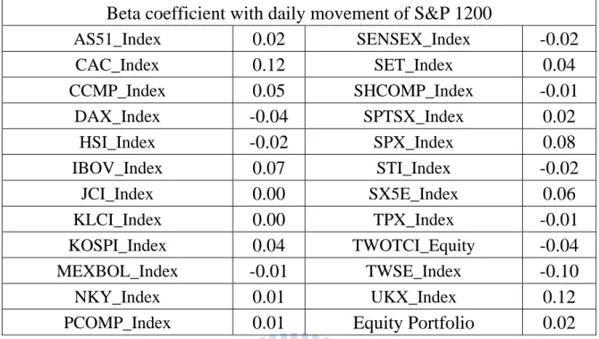
First, we calculate the beta between each equity trading strategies in Single Moving Average with S&P 1200 daily movement behavior. Second, we do the
“Tests of Significance” by Z-Test in this strategy. Hypotheses for our test is as follows: {H0 :μ =μ0, H1:μ >μ0}, μ0 is the mean of asset daily movement return
Beta coefficient with daily movement of S&P 1200
AS51_Index0.02
SENSEX_Index-0.02
CAC_Index0.12
SET_Index0.04
CCMP_Index0.05
SHCOMP_Index-0.01
DAX_Index-0.04
SPTSX_Index0.02
HSI_Index-0.02
SPX_Index0.08
IBOV_Index0.07
STI_Index-0.02
JCI_Index0.00
SX5E_Index0.06
KLCI_Index0.00
TPX_Index-0.01
KOSPI_Index0.04
TWOTCI_Equity-0.04
MEXBOL_Index-0.01
TWSE_Index-0.10
NKY_Index0.01
UKX_Index0.12
PCOMP_Index
0.01 Equity
Portfolio 0.02
Table 8: The beta sheet of single MA strategy in equity market. The result means that our trading strategy has low linear correlation with the benchmark index which is chosen as S&P 1200.
The probability we don't reject
H0TWOTCI_Equity 0.00% CCMP_Index 26.37% KLCI_Index 0.02% SX5E_Index 29.27% SHCOMP_Index 0.23% NKY_Index 35.20% STI_Index 1.77% DAX_Index 43.69% SENSEX_Index 5.45% SPX_Index 47.00% HSI_Index 9.66% AS51_Index 50.90% PCOMP_Index 9.89% CAC_Index 53.59% JCI_Index 11.28% SET_Index 57.66% TPX_Index 14.61% IBOV_Index 57.95% TWSE_Index 14.95% UKX_Index 62.39% SPTSX_Index 17.91% MEXBOL_Index 70.51% KOSPI_Index 21.45%
Table 9: The P-value sheet of single MA with buy&hold, which states that our trading strategy’ mean of return is usually higher than buy&hold one in terms of Z-test, but there are 6 indices p value larger than 0.5 which means theμ in the particular strategy may not be larger than μ0 or even worse.
3.2.2 Dual Moving Average
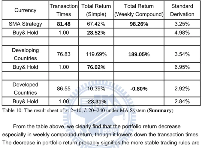
In this part, we replace SMA from 1 to 2~10 as the currency market strategy. The method is addressed by Olson in currency market. Now we verify it in equity market. Currency Transaction Times Total Return (Simple) Total Return (Weekly Compound) Standard Derivation SMA Strategy 81.48 67.42% 98.26% 3.25% Buy& Hold 1.00 28.52% 4.98% Developing Countries 76.83 119.69% 189.05% 3.54% Buy& Hold 1.00 76.02% 6.95% Developed Countries 86.55 10.39% -0.80% 2.92% Buy& Hold 1.00 -23.31% 2.84%
Table 10: The result sheet of s: 2~10, l: 20~240 under MA System (Summary)
From the table above, we clearly find that the portfolio return decrease
especially in weekly compound return, though it lowers down the transaction times. The decrease in portfolio return probably signifies the more stable trading rules are not the promise of better return. We are losing our portfolio return as decreasing the transaction times. However, this trading strategy return still beats the buy&hold with a distance(annualized rate of 6.84%).
3.2.3 Combination of Single Moving average with Stochastic oscillator(MK)
As in the currency market, we try the MK model in equity market. The combining logic is still the same as set in Currency strategy:
① Parameter set: 『s:1, l:20~240 under MA System』and 『n:10~20, s:3~10,
l:3~10 under SO System』
② Go long at if ( > LMA) and ( < → > ) unless (K<25) for
two consecutive trading days.
c t
P c t
P Kt−1 Dt−1 Kt Dt
③ Go Short at if ( < LMA) and ( > → < ) unless (K>75) for
two consecutive trading days.
c t
P c t
P Kt−1 Dt−1 Kt Dt
④ In any other situation, we just keep our position.
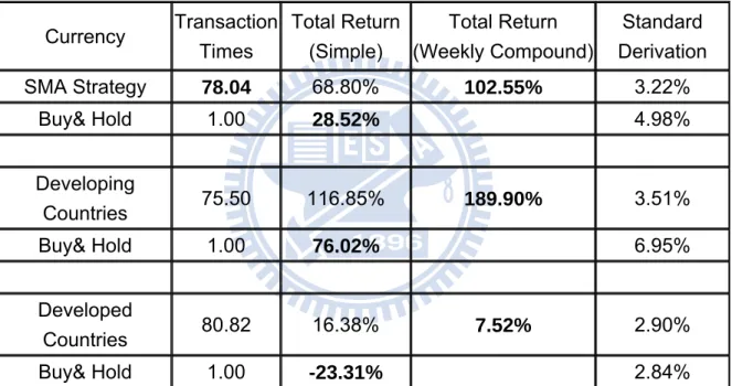
Currency Transaction Times Total Return (Simple) Total Return (Weekly Compound) Standard Derivation SMA Strategy 78.04 68.80% 102.55% 3.22% Buy& Hold 1.00 28.52% 4.98% Developing Countries 75.50 116.85% 189.90% 3.51% Buy& Hold 1.00 76.02% 6.95% Developed Countries 80.82 16.38% 7.52% 2.90% Buy& Hold 1.00 -23.31% 2.84%
Table 11:The result sheet of MK model in equity market (Summary)
From the table above, we find that the portfolio return of MK model still
decrease as the Dual Moving Average strategy in weekly compound return, though it lowers down the transaction times. The reason why the step of stabilization in our trading strategy eventually loses return in equity market probably can point to “Volatility of the Asset.” We shall discuss the issue later. Nevertheless, return of this trading strategy still beats the buy&hold with an annualized rate of 7.17%. ThenWe do some statistics as above. First, we calculate the beta between each equity trading strategies in MK model with S&P 1200 daily movement behavior. Then we
do the “Tests of Significance” by Z-Test. Hypotheses for our test is as follows: {H0 :μ =μ0, H1:μ >μ0}, μ0 is the mean of asset daily movement return
Beta coefficient with daily movement of S&P 1200
AS51_Index0.05
SENSEX_Index-0.01
CAC_Index0.15
SET_Index0.04
CCMP_Index0.02
SHCOMP_Index-0.05
DAX_Index-0.05
SPTSX_Index0.00
HSI_Index-0.02
SPX_Index0.09
IBOV_Index0.08
STI_Index-0.04
JCI_Index0.00
SX5E_Index0.07
KLCI_Index0.01
TPX_Index0.02
KOSPI_Index0.05
TWOTCI_Equity-0.06
MEXBOL_Index0.02
TWSE_Index-0.11
NKY_Index-0.02
UKX_Index0.14
PCOMP_Index
0.02 Equity
Portfolio 0.02
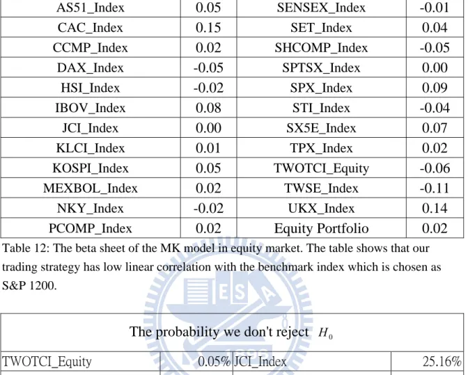
Table 12: The beta sheet of the MK model in equity market. The table shows that our trading strategy has low linear correlation with the benchmark index which is chosen as S&P 1200.
The probability we don't reject
H0TWOTCI_Equity 0.05% JCI_Index 25.16% SHCOMP_Index 0.55% TWSE_Index 27.36% KLCI_Index 1.17% SPX_Index 37.64% STI_Index 15.80% SX5E_Index 37.66% PCOMP_Index 15.83% SET_Index 44.90% SPTSX_Index 16.19% UKX_Index 49.87% HSI_Index 17.18% AS51_Index 52.06% NKY_Index 17.43% KOSPI_Index 55.54% TPX_Index 18.09% IBOV_Index 64.00% DAX_Index 19.92% CCMP_Index 70.14% SENSEX_Index 22.52% MEXBOL_Index 89.01% CAC_Index 22.73%
Table 13: The sheet states that our trading strategy’ mean of return is usually higher than buy&hold one in terms of Z-test, but there are 5 indices p value larger than 0.5 which means theμ in the particular strategy may not be larger than μ0 or even worse.
3.3 Discussion on the appropriateness of our trading criteria
3.3.1 The trade off between stabilization and efficiencyThe reason why “step of stabilization” loses return in equity market may
originate in the volatility. In a stable market, meaning the asset has low volatility, the step of stabilization can decrease the transaction costs without losing return or even increasing it due to filtering out noisy signal. We can take TWD as an example, the standard deviation of TWD is 0.57% which is lowest in all currency and equity market we observing. Recalling from the MK Model, we request the signal must
keep two consecutive trading days, and then we go “long” or “short” our position. The incorporation of “Stochastic Oscillator” and “two consecutive days (consecutive
set=2)” are the methods we try to stabilize the trading signal. The figure below
explains it.
Figure.6: TWD performance under MK model with consecutive set=2
From the two figures above, we can clearly observe the rule of “consecutive set=5” doesn’t worsen the return, though “consecutive set=5” is a little unrealistic and clumsy. The same situation happens in RUB, which has volatility of “0.59%”
Figure.8: RUB performance under MK model with consecutive set=2
Figure.9: RUB performance under MK model with consecutive set=5
On the contrary, TWOTCI is volatile index in our observing samples. Our stabilizing rules lower down the return sharply.
Figure.10: TWOTC_Index performance under MK model with no consecutive set
Figure.11: TWOTC_Index performance under MK model consecutive set=2. Notice that the weekly compound return decreased from about 800% to about 400%, which shows that the delay rule does lose good timing for entering or exiting position.
To be true, the relationship between 『volatility of asset』 and 『stabilization of trading rule』 are not “if and only if”, but from charts above, it appears to express that the more volatile in financial market, the more we should pay attention to the stabilizing criterion we use. Nevertheless, this issue maybe can have further study in the future.
3.3.2 The choice of Back-test and Forecasting Period.
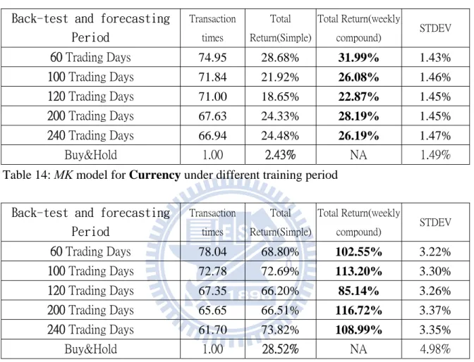
It should be a critical issue that “Does our return change tremendously as we alter the training period? In fact, our choice of 60-trading days is just one of the selections in practical financial industry. We shall examine it now. In the table below, we will show the portfolio return in MK Model with different training period.
Back-test and forecasting Period Transaction times Total Return(Simple) Total Return(weekly compound) STDEV 60 Trading Days 74.95 28.68% 31.99% 1.43% 100 Trading Days 71.84 21.92% 26.08% 1.46% 120 Trading Days 71.00 18.65% 22.87% 1.45% 200 Trading Days 67.63 24.33% 28.19% 1.45% 240 Trading Days 66.94 24.48% 26.19% 1.47% Buy&Hold 1.00 2.43% NA 1.49%
Table 14: MK model for Currency under different training period
Back-test and forecasting Period Transaction times Total Return(Simple) Total Return(weekly compound) STDEV 60 Trading Days 78.04 68.80% 102.55% 3.22% 100 Trading Days 72.78 72.69% 113.20% 3.30% 120 Trading Days 67.35 66.20% 85.14% 3.26% 200 Trading Days 65.65 66.51% 116.72% 3.37% 240 Trading Days 61.70 73.82% 108.99% 3.35% Buy&Hold 1.00 28.52% NA 4.98%
Table 15: MK model for Equity under different training period
It apparently reveals that the change of training period doesn’t result in a huge change in our return, at least, every weekly compound return are obviously larger than buy&hold strategy.
3.4 The issue of “Reflexivity”
Before we keep go on, we need to inspect on the concept of the important financial theory “Reflexivity”. The first and the most important one who address “The theory of Reflexivity” in financial market is George Soros whose writings focus heavily on the concept of reflexivity, where the biases of individuals enter into market transactions, potentially changing the perception of fundamentals of the economy. Soros argues that such transitions in the perceptions of fundamentals of the economy are typically marked by disequilibrium rather than equilibrium, and that
the conventional economic theory of the market (EMH) does not apply in these situations.
Reflexivity is based on three main ideas
1. Reflexivity is best observed under special conditions where investor bias grows and spreads throughout the investment arena. Examples of factors that may give rise to this bias include (a) equity leveraging or (b) the trend-following habits of speculators.
2. Reflexivity appears intermittently since it is most likely to be revealed under certain conditions; i.e., the equilibrium process's character is best considered in terms of probabilities.
3. Investors' observation of and participation in the capital markets may at times influence valuations AND fundamental conditions or outcomes.
As to the application of “Reflexivity” on technical analysis, Soros has the point of view described below. Trend following such as MA is an important element of Soros’ strategy. He views upticks and downticks as important predictors of price trends because they provide information about the strength of supply and demand. However, technical analysis is limited by the fact that financial markets are not closed systems. The market is always in interaction with the much wider economic system and constantly receives input from the outside world. This means that a trader cannot blindly assume that predicting the future can be achieved with a mechanistic reworking of past data, even in the probabilistic sense! Technical approaches that calculate probabilities on the basis of past experience lose the context in which each particular instance occurs. This is why traders always need to use their bodily sense of the current situation,
The starting point in Soros’ approach is the participants’ bias. The participants’ bias gives rise to trends, which Soros at first follows. He then looks for the flaw in the prevailing rationale behind the trend. Of course, market participants have different views and base their decisions on different approaches. It must be remembered, however, that for a strong trend to form, there needs to be some consensus among different groups of participants such as fundamentally oriented participants and technical trend followers. Finding the flaw in the market’s
hypothesis puts him ahead of the curve – he still follows the trend, but is on the lookout for what would make it reverse.
In reflexive situations, the market trend at first supports the bias. Bias and trend reinforce one another. But the trend also has unintended consequences, affecting economic relationships which the conventional view is not taking into account. Again, market action takes place within an intricate web of interlocking economic
processes, not within a vacuum. At this underlying level, the market’s action is creating an effect that eventually makes the trend unsustainable.
3.4.1 CART analysis on stochastic oscillator
From the theory above, we realize that why the traditional trading indicators brought up in the past has gradually failed. The classical example of this theory on technical analysis is “Stochastic Oscillator” addressed by George Lane in 1956.
Figure.12: KD(9,3,3) on S&P 500 in 1953~2008
The SO is addressed in 1956, and we can see from the chart that this method
had continuously made excess profit than the benchmark index for 20 years. The reason why the indicator could sustain 20-years’ excess return probably is the “Bias and trend reinforce one another” on reflexivity theory; however, with the
continuously accumulated perception of this indicator, the SO started to fail in 1983.
I think that could be an understanding of reflexivity on SO indicator.
Since the KD (9,3,3) is worldwide watched in the financial industry and market has produced reflexivity on the indicator, can we take advantage of it? Our
attempting method is CART and we try to use the ability of classification in it to form a trading strategy. Our trading process is set as follows:
① Generate an sheet which includes in a pair data of “(K-D) value” and “Next-term asset return.”
② Then we use CART to help us classify the relation between (K-D) value with the next-term asset return in a yearly basis.
③ In order to suit for CART in training desirable classification, we only focus on absolute scalars(that means we will alter the sign in “Next-term Return” when “(K-D) value” are negative) and calculate data in 3-days as bases
④ Finally, we use the prior year’ classification table, which is composed of about 240 samples, on the next year and recursively run this procedure on 2001~2008. ⑤ Besides, due to its high transaction times by nature of our trading rules, we only choose countries which exists contracts of future trading and the transaction cost is considered as 0.05%. When return in classification table is less than 0.05%, We just ignore the zone and don’t make any trade.
The figure below shows an example of CART on Dow Jones Industrial Average in 2007 and the return sheet of all equity indices is next to it.
Figure.13: Classification table by CART on INDU in 2007. In this table, we train the (k-d) value in absolute scalar with an yearly basis.
Transaction times Total Return(Simple) Total Return(Compound) UKX_Index 249 57.51% 61.38% SPX_Index 288 81.25% 108.69% INDU_Index 307 59.79% 68.47% CCMP_Index 317 -6.05% -28.40% DAX_Index 280 -71.74% -69.62% CAC_Index 286 -98.42% -79.94% SX5E_Index 299 99.41% 140.50% AS51_Index 277 76.37% 111.11% SPTSX_Index 296 12.89% 0.74% NKY_Index 300 109.05% 165.26% HSI_Index 286 41.64% 18.03% TWSE_Index 308 -27.99% -46.54% KOSPI_Index 273 -114.12% -86.06% STI_Index 265 59.70% 18.19% IBOV_Index 277 -16.01% -43.44% MEXBOL_Index 306 -181.15% -99.85% CART on KD(9,3,3) 288.38 5.13% 14.91% Original KD(9,3,3) 371.25 -70.64% -46.47%
Table 16: The return sheet of CART on KD(9,3,3).
From the table above, we have the following conclusions:
1. Return of CART on KD(9,3,3) obviously improves the original KD strategy, but mean of return is just slightly higher than zero. The probable reasons could be the as high as the original frequent transaction times and the seriously bad performance on Mexico index.
2. CART does improve the return a lot in developed countries. It maybe mean that the method actually catch the “reflexive effect of KD(9,3,3) on developed countries.”
3. The high volatility between each indices may indicate that our trading rules should be refined to a more stable one.
Due to the originality of this method, this strategy surely needs to be revised or given further study on it. Nevertheless, KD(9,3,3) literally make an progress on the concept of reflexivity characterized by CART.
3.4.2 The selection of price in entering and exiting position
For the institutional investors, it is more likely that we use next day’s price as the entering or exiting price rather than the close price for the sake of convenience and risk control. In this section, we will replace the price used in calculating return from close price: to the average of the next day’s high and low one:
0.5*( + ). Due to change in price we use, we shall apply the same rule when our program executes back-testing procedure. The comparing tables are as follows:
c t P h t P+1 l t P+1
Single Moving Average
Transaction times Total Return(Simple) Total Return(weekly compound) STDEV
60 Trading Days 141.37 9.05% 9.02% 1.49% 100 Trading Days 123.11 9.09% 10.21% 1.49% 120 Trading Days 115.16 14.24% 14.16% 1.48% 200 Trading Days 112.47 8.73% 6.57% 1.51% 240 Trading Days 113.37 10.81% 10.79% 1.49% Average 10.39% 10.15% 60 Trading Days 139.53 12.22% 11.49% 1.38% 100 Trading Days 124.16 9.49% 9.55% 1.40% 120 Trading Days 118.74 11.08% 10.10% 1.39% 200 Trading Days 112.42 11.08% 9.35% 1.39% 240 Trading Days 109.89 13.45% 12.29% 1.39% Average 11.46% 10.56%
Table 17: The comparison sheet of different used price in single MA. The upper section is outcome of close price, and the lower one is calculated by next day price.
MK model in Currency
Transaction times Total Return(Simple) Total Return(weekly compound) STDEV
60 Trading Days 74.95 28.68% 31.99% 1.43% 100 Trading Days 71.84 21.92% 26.08% 1.46% 120 Trading Days 71 18.65% 22.87% 1.45% 200 Trading Days 67.63 24.33% 28.19% 1.45% 240 Trading Days 66.94 24.48% 26.19% 1.47% Average 23.61% 27.06% 60 Trading Days 74.47 26.31% 28.61% 1.35% 100 Trading Days 71.16 24.47% 27.27% 1.36% 120 Trading Days 66.26 28.11% 31.73% 1.35% 200 Trading Days 66.11 19.50% 21.38% 1.37% 240 Trading Days 64.58 23.71% 27.35% 1.36% Average 24.42% 27.26%
Table 18: The comparison sheet of different used price in MK model
Single Moving Average
60 Trading Days 133.30 73.61% 164.92% 3.20% 100 Trading Days 125.52 65.18% 132.58% 3.28% 120 Trading Days 115.83 81.85% 136.36% 3.26% 200 Trading Days 112.91 87.34% 208.93% 3.30% 240 Trading Days 106.96 96.35% 220.83% 3.36% Average 80.87% 172.72% 60 Trading Days 131.83 48.21% 74.61% 3.11% 100 Trading Days 117.35 59.30% 98.57% 3.16% 120 Trading Days 108.43 54.70% 74.87% 3.16% 200 Trading Days 101.48 83.92% 140.89% 3.18% 240 Trading Days 101.91 74.26% 116.08% 3.32% Average 64.08% 101.01%