Thermal fluctuation correction to magnetization and specific heat of vortex solids
in type-II superconductors
Dingping Li*and Baruch Rosenstein†
National Center for Theoretical Sciences and Electrophysics Department, National Chiao Tung University, Hsinchu 30050, Taiwan, Republic of China
共Received 21 May 2001; published 19 December 2001兲
A systematic calculation of magnetization and specific heat contributions due to fluctuations of vortex lattice in strongly type-II superconductors to precision of 1% is presented. We complete the calculation of the two loop low temperature perturbation theory by including the umklapp processes. Then the Gaussian variational method is adapted to calculation of thermodynamic characteristics of the two-dimensional and the three-dimensional vortex solids in high magnetic field. Based on it as a starting point for a perturbation theory we calculate the leading correction providing simultaneously an estimate of precision. The results are compared to existing nonperturbative approaches.
DOI: 10.1103/PhysRevB.65.024514 PACS number共s兲: 74.60.⫺w, 74.40.⫹k, 74.25.Ha, 74.25.Dw
I. INTRODUCTION
Existence of a vortex lattice in type-II superconductors in magnetic field was predicted by Abrikosov and subsequently observed in various materials ranging from metals to high Tc
cuprates. In the original treatment the mean field Ginzburg– Landau 共GL兲 theory, which neglects thermal fluctuations of the vortex matter, was used. Thermal fluctuations are ex-pected to play a much larger role in high Tcsuperconductors than in the low temperature ones, because the Ginzburg pa-rameter Gi characterizing fluctuations is much larger.1In ad-dition, the presence of a strong magnetic field and strong anisotropy in superconductors like BSCCO effectively re-duces their dimensionality, thereby further enhancing effects of thermal fluctuations. Under these circumstances fluctua-tions make the lattice softer, in turn influencing various physical properties like magnetization and specific heat. Eventually it leads to melting of the vortex lattice into a vortex liquid far below the mean field phase transition line.2,1 The first order melting transition was clearly demonstrated in both magnetization3 and specific heat experiments.4 To de-velop a theory of these fluctuations, even in the case of low-est Landau level 共LLL兲, corresponding to regions of the phase diagram ‘‘close’’ to Hc2, is a very nontrivial task and
several different approaches were developed.
At the high temperature end共namely far above the mean field transition temperature and thereby in the ‘‘vortex liq-uid’’ phase兲 one can develop the traditional ‘‘loop’’ expan-sion. Since the melting line lies below the mean field line, Thouless and Ruggeri5,6 proposed a perturbative expansion which can be defined below this line. It contains one loop together with a certain class of higher loop diagrams 共‘‘bubbles’’兲 and therefore is ‘‘nonperturbative.’’ It was shown in field theory that summation of all the bubble dia-grams is equivalent to the Gaussian variational approach.7In this approach one searches for a ‘‘Gaussian’’ state having the lowest energy. The series provides accurate results at high temperatures, but become inapplicable for LLL dimension-less temperature aT⬃(T⫺Tm f(H))/(TH)1/2 smaller than 2
in 2D and for aT⬃(T⫺Tm f(H))/(TH)2/3 smaller than 1 in
3D, both quite far above the melting line. Generally, attempts to extend the theory to lower temperature by Pade´ extrapo-lation were not successful.8It is in fact doubtful whether the perturbative results based on Gaussian approximation assum-ing translational invariant liquid state should be attempted at low aT.
In Ref. 9, it was shown that below aT⬍⫺5 different Gaussian states which are no longer translationally invariant have lower energy. We will present the detailed calculation here 共optimized perturbation theory was used to study for liquid state, see Refs. 9 and 10兲. It is in general a very non-trivial problem to find an inhomogeneous solutions of the corresponding ‘‘gap equation’’共see Sec. IV兲. However, using previous experience with low temperature perturbation theory,11,12 the problem can be significantly simplified and solved using rapidly convergent ‘‘modes’’ expansion. A con-sistent perturbation theory should start from these states.13 We then generalize the approach of Ref. 5 by setting up a perturbation theory around the Gaussian Abrikosov lattice state.
Magnetization and specific heat contributions due to vor-tex lattices are calculated in perturbation theory around this state to next to leading order. This allows to estimate the precision of the calculation. It is the worst, about 1%, near the melting point at aT⫽⫺10 and becomes better for lower
aT. At low temperature the result is consistent with the first
principles low temperature perturbation theory advanced re-cently to the two loop order.11,12The previous two loop cal-culation is completed by including the Umklapp processes. One can make several definitive qualitative conclusions us-ing the improved accuracy of the results. The LLL scaled specific heat monotonously rises from its mean field value of 1/A at aT⫽⫺⬁ to a slightly higher value of 1.05/Awhere
A⫽1.16 is Abrikosov parameter. This is at variance with
theory Ref. 14 which uses completely different ideas and has a freedom of arbitrarily choosing certain parameters on a 2% precision level. Although we calculate the contribution of the LLL only, corrections due to higher Landau levels calculated earlier in Refs. 15 and 16 using a less sophisticated method can be included.
The paper is organized as follows. The model is defined in Sec. II. In Sec. III a brief summary of existing results and Umklapp corrected two loop perturbative results in both 2D and 3D are given. Gaussian approximation and the mode expansion used is described in Sec. IV. The basic idea of expansion around the best Gaussian state is explained in Sec. V. The leading corrections are calculated. Results are pre-sented and compared with perturbation theory and other theories in Sec. VI together with conclusions.
II. MODELS
To describe fluctuations of order parameter in thin films or layered superconductors one can start with the Ginzburg– Landau free energy
F⫽Lz
冕
d2x ប2 2mab 兩D兩2⫺a兩兩2⫹b⬘
2 兩兩 4, 共1兲 where A⫽(By,0) describes a constant magnetic field 共con-sidered nonfluctuating兲 in Landau gauge and covariant de-rivative is defined by D⬅“⫺i(2/⌽0)A, ⌽0⬅hc/e*. For strongly type-II superconductors like the high Tc cuprates(⬃100) and not too far from Hc2 共this is the range of
interest in this paper, for the detailed discussion of the range of applicability see Ref. 15兲 magnetic field is homogeneous to a high degree due to superposition from many vortices. For simplicity we assume a(T)⫽␣Tc(1⫺t), t⬅T/Tc,
al-though this temperature dependence can be easily modified to better describe the experimental Hc2(T). The thickness of a layer is Lz.
Throughout most of the paper we will use the coherence length ⫽
冑
ប2/(2mab␣Tc) as a unit of length and
dHc2共Tc兲
dT Tc⫽ ⌽0 22
as a unit of magnetic field. After the order parameter field is rescaled as 2→(2␣Tc/b
⬘
)2, the dimensionless freeen-ergy 共the Boltzmann factor兲 is F T⫽ 1
冕
d2x冋
1 2兩D兩 2⫺1⫺t 2 兩兩 2⫹1 2兩兩 4册
. 共2兲 The dimensionless coefficient describing the strength of fluc-tuations is ⫽冑
2 Gi2t⫽ mabb⬘
2ប2␣Lzt, Gi⬅ 1 2冉
32e222Tc c2h2Lz冊
2 , 共3兲 where Gi is the Ginzburg number in 2D . When (1⫺t ⫺b)/12bⰆ1, the lowest Landau level 共LLL兲 approximation can be used.15 The model then simplifies due to the LLL constraint, ⫺(D2/2)⫽(b/2), rescaling x→x/冑
b, y→y/
冑
b, and兩兩2→兩兩2冑
b/4, one obtains f⫽ 1 4冕
d 2x冋
a T兩兩2⫹ 1 2兩兩 4册
, 共4兲where the 2D LLL reduced temperature
aT⬅⫺
冑
4 b
1⫺t⫺b
2 共5兲
is the only parameter in the theory.17,5
For 3D materials with asymmetry along the z axis the GL model takes the form
F⫽
冕
d3x ប 2 2mab冏
冉
“⫺ ie* បc A冊
冏
2 ⫹ ប 2 2mc 兩z兩 2 ⫹a兩兩2⫹b⬘
2 兩兩 4 共6兲which can be again rescaled into
f⫽F T⫽ 1
冕
d3x冋
1 2兩D兩 2⫹1 2兩z兩 2⫺1⫺t 2 兩兩 2⫹1 2兩兩 4册
, 共7兲 by x→x, y→y , z→z/␥1/2, 2→(2␣Tc/b⬘
)2, where␥⬅mc/mab is anisotropy. The Ginzburg number is now
given by Gi⬅1 2
冉
32e22Tc␥1/2 c2h2冊
2 . 共8兲Within the LLL approximation, and rescaling x→x/
冑
b, y→y/
冑
b, z→z(b/4冑
2)⫺1/3, 2→(b/4冑
2)2/32, the dimensionless free energy becomesf⫽ 1 4
冑
2冕
d 3x冋
1 2兩z兩 2⫹a T兩兩2⫹ 1 2兩兩 4册
. 共9兲 The 3D reduced temperature isaT⫽⫺
冉
b 4冑
2冊
⫺2/3 1⫺t⫺b 2 . 共10兲From now on we work with rescaled quantities only and relate them to measured quantities in Sec. V.
III. PERTURBATION THEORIES AND EXISTING NONPERTURBATIVE RESULTS
A variety of perturbative as well as nonperturbative meth-ods have been used to study this seemingly simple model. There are two phases. Neglecting thermal fluctuations, one obtains the lowest energy configuration⫽0 for aT⬎0 and
⫽
冑
⫺ aT A , ⫽冑
2冑
a⌬ l⫽⫺⬁兺
⬁ exp再
i冋
l共l⫺1兲 2 ⫹ 2 a⌬lx册
⫺12冉
y⫺2 a⌬l冊
2冎
共11兲for aT⬍0, where a⌬⫽
冑
4/冑
3 is the lattice spacing in ourunits andA⫽1.16.
A. High temperature expansion in the liquid phase Homogeneous ‘‘vortex liquid’’ phase 共which is not sepa-rated from the ‘‘normal’’ phase by a transition兲 has been studied using high temperature perturbation theory by Thou-less and Ruggeri.5 Unfortunately these asymptotic series 共even pushed to a very high orders18兲 are applicable only when aT⬎2. In order to extend the results to lower aT,
attempts have been made to Pade´ resum the series6imposing a constraint that the result matches the Abrikosov mean field as aT→⫺⬁. However, if no matching to the limit is
im-posed, the perturbative results cannot be significantly improved.8 Experiments,3,4 Monte Carlo simulations19 and nonperturbative Bragg chain approximation20 all point out that there is a first order melting transition around aT
⫽⫺12. If this is the case it is difficult to support such a constraint.
B. Low temperature perturbation theory in the solid phase: Umklapp processes
Recently a low temperature perturbation theory around Abrikosov solution Eq.共11兲 was developed and shown to be consistent up to the two loop order.11,12,16 Since we will use in the present study the same basis and notations and also will compare to the perturbative results we recount here a few basic expressions. The order parameter field is divided into a nonfluctuating共mean field兲 part and a small fluctuation
共x兲⫽
冑
⫺a TA 共x兲⫹共x兲.
共12兲 The field can be expanded in a basis of quasi momentum eigenfunctions on LLL in 2D: k⫽
冑
2冑
a⌬l⫽⫺⬁兺
⬁ exp再
i冋
l共l⫺1兲 2 ⫹ 2共x⫺ky兲 a⌬ l⫺xkx册
⫺12冉
y⫹kx⫺ 2 a⌬l冊
2冎
. 共13兲Then we diagonalize the quadratic term of free energy Eq. 共4兲 to obtain the spectrum. Instead of the complex field , two ‘‘real’’ fields O and A will be used,
共x兲⫽ 1
冑
2冕
k exp关⫺ik/2兴k共x兲 共冑
2兲2 共Ok⫹iAk兲, 共14兲 *共x兲⫽冑
1 2冕
k exp关ik/2兴k*共x兲 共冑
2兲2 共O⫺k⫺iA⫺k兲, where ␥k⫽兩␥k兩exp关ik兴 and definition of ␥k 共and all otherdefinitions of functions兲 can be found in Appendix A. The eigenvalues found by Eilenberger in Ref. 21 are
⑀A共k兲⫽⫺aT
冉
⫺1⫹ 2 A k⫺ 1 A 兩␥k兩冊
, 共15兲 ⑀O共k兲⫽⫺aT冉
⫺1⫹ 2 A k⫹ 1 A 兩␥k兩冊
.where k is defined in Appendix A. In particular, when k
→0 共Ref. 22兲,
⑀A⬇0.12兩aT兩兩k兩4. 共16兲
The second excitation mode ⑀O has a finite gap. The free
energy to the two loop order was calculated in Ref. 12, how-ever the Umklapp processes were not included in some two loop corrections. These processes correspond to momentum nonconserving 共up to integer times inverse lattice constant兲 four leg vertices 关see Appendix A, Eq. 共A2兲兴. We therefore recalculated these coefficients. The result in 2D is关see Figs. 1共a兲 and 1共b兲兴 feff 2D⫽⫺ aT2 2A ⫹2 log兩aT兩 42⫺ 19.9 aT2 ⫹cv, 共17兲 where cv⫽
具
log关(⑀A(k)⑀O(k)/aT2
兴
典
⫽⫺2.92. In 3D, similar calculation共extending the one carried in Ref. 11 to Umklapp processes兲 gives feff 3D⫽⫺ aT2 2A ⫹2.848兩aT兩1/2⫹ 2.4 aT . 共18兲 C. Nonperturbative methodsFew nonperturbative methods have been attempted. Te-sanovic and co-workers14 developed a method based on an approximate separation of the two energy scales. The larger contribution 共98%兲 is the condensation energy, while the smaller one共2%兲 describes motion of the vortices. The result for energy in 2D is feff⫽⫺ aT2U2 4 ⫺ aT2U 2
冑
U2 4 ⫹ 2 aT2⫹2 arc sinh冋
aTU 2冑
2册
, 共19兲 U⫽1 2冋
1冑
2⫹ 1冑
A ⫹tanh冋
aT 4冑
2⫹ 1 2册冉
1冑
2⫺ 1冑
A冊
册
.Corresponding expressions in 3D were also derived. No melting phase transition is seen since it belongs to the 2% which cannot be accounted for within this approach. There exist several Monte Carlo 共MC兲 simulations of the system.19 The expression Eq. 共19兲 agrees quite well with high temperature perturbation theory and MC simulations and has been used to fit both magnetization and specific heat experiments,4 but only the mean field level agrees with low temperature perturbation theory. Expanding Eq.共19兲 in 1/aT,
one obtains an opposite sign of the one loop contribution, see Fig. 1共a兲 and discussion in Sec. VI.
Other interesting nonperturbative methods include the 1/N expansion23,24in which the GL model is generalized to
an N component theory and the phenomenological ‘‘Bragg chain fluctuation approximation’’20 based on the elasticity theory of the vortex matter.
IV. GAUSSIAN VARIATIONAL APPROACH A. General anzatz
Gaussian variational approach originated in quantum me-chanics and has been developed in various forms and areas of physics.25,26In quantum mechanics it consists of choosing a Gaussian wave function which has the lowest energy ex-pectation value. When fermionic fields are present the ap-proximation corresponds to BCS or Hartree–Fock varia-tional state. In scalar field theory one optimizes the quadratic part of the free energy
f⫽
冕
⫺1 2 aD⫺1a⫹V共a兲 ⫽冕
1 2共 a⫺va兲G⫺1ab共b⫺vb兲⫹V˜共G,a兲 ⫽K⫹V˜. 共20兲To obtain ‘‘shift’’va and ‘‘width of the Gaussian’’ G, one minimizes the Gaussian effective free energy,26 which is an exact upper bound on the energy共see proof in Ref. 25兲. The result of the Gaussian approximation can be thought of as resummation of all the ‘‘cacti’’ or loop diagrams.5,7 Further corrections will be obtained in Sec. V by inserting this solu-tion for G and taking more terms in the expansion of Z.
B. 2D Abrikosov vortex lattice
In our case of one complex field one should consider the most general quadratic form
K⫽
冕
x,y共*共x兲⫺v
*共x兲兲G⫺1共x,y兲共共y兲⫺v共y兲兲⫹共 ⫺v共x兲兲H*共⫺v共x兲兲⫹共*⫺v*共x兲兲H共*⫺v*共x兲兲.
共21兲 Assuming hexagonal symmetry 共a safe assumption for the present purpose兲, the shift should be proportional to the mean field solution Eq.共12兲, v(x)⫽v(x), with a constantv
taken real thanks to global U共1兲 gauge symmetry. On LLL, as in perturbation theory, we will use variables Ok and Ak defined in Eq.共14兲 instead of(x),
共x兲⫽v共x兲⫹
冑
1 22冕
kexp
冋
⫺ik2
册
k共x兲共Ok⫹iAk兲. 共22兲 The phase defined after Eq.共14兲 is quite important for sim-plification of the problem and was introduced for future con-venience. The most general quadratic form isK⫽ 1 8
冕
kOkGOO⫺1共k兲O⫺k⫹AkGAA⫺1共k兲A⫺k
⫹OkGOA⫺1共k兲A⫺k⫹AkGOA⫺1共k兲O⫺k, 共23兲
with matrix of functions G(k) on Brillouin zone to be deter-mined together with the constant v by the variational
prin-ciple. The corresponding Gaussian free energy is
fGauss⫽aTv2⫹ A 2 v 4⫺2⫺
具
log关共4兲2det共G兲兴典
k ⫹具
aT共GOO共k兲⫹GAA共k兲兲⫹v2关共2k⫹兩␥k兩兲GOO共k兲 ⫹共2k⫺兩␥k兩兲GAA共k兲兴典
k具
k⫺l关GOO共k兲⫹GAA共k兲兴 ⫻关GOO共l兲⫹GAA共l兲兴典
k,l⫹ 1 2A兵具
兩␥k兩共GOO共k兲 ⫺GAA共k兲兲典
2⫹4具
兩␥k兩GOA共k兲典
k 2 其, 共24兲where
具
•••典
k denotes average over the Brillouin zone. Theminimization equations are
v2⫽⫺aT A⫺ 1 A
具
共2k⫹兩␥k兩兲GOO共k兲 ⫹共2k⫺兩␥k兩兲GAA共k兲典
k, 共25兲 关G共k兲⫺1兴 OO⫽aT⫹v2共2k⫹兩␥k兩兲 ⫹冓
冉
2k⫺l⫹ 兩␥k兩兩␥l兩 A冊
GOO共l兲 ⫹冉
2k⫺l⫺ 兩␥k兩兩␥l兩 A冊
GAA共k兲冔
l , 共26兲 关G共k兲⫺1兴 AA⫽aT⫹v2共2k⫺兩␥k兩兲 ⫹冓
冉
2k⫺l⫹ 兩␥k兩兩␥l兩 A冊
GAA共l兲 ⫹冉
2k⫺l⫺ 兩␥k兩兩␥l兩 A冊
GOO共k兲冔
l , 共27兲 关G共k兲⫺1兴 OA⫽⫺ GOA共k兲 GOO共k兲GAA共k兲⫺GOA共k兲2 ⫽4兩␥k兩 A具
兩␥l兩GOA共l兲典
l. 共28兲These equations look quite intractable, however they can be simplified. The crucial observation is that after we have in-serted the phase exp关⫺ik/2兴 in Eq. 共22兲 using our experi-ence with perturbation theory, GAO appears explicitly only
on the right-hand side of the last equation. It also implicitly appears on the left-hand side due to a need to invert the matrix G. Obviously GOA(k)⫽0 is a solution and in this
case the matrix diagonalizes. However general solution can be shown to differ from this simple one just by a global
gauge transformation. Subtracting Eq.共26兲 from Eq. 共27兲 and using Eq.共28兲, we observe that matrix G⫺1 has the form
G⫺1⬅
冉
EO共k兲 EOA共k兲 EOA共k兲 EA共k兲冊
⫽冉
E共k兲⫹⌬⌬ 1兩␥k兩 ⌬2兩␥k兩 2兩␥k兩 E共k兲⫺⌬1兩␥k兩冊
,where⌬1,⌬2 are constants. Substituting this into the Gauss-ian energy one finds that it depends on⌬1,⌬2 via the com-bination ⌬⫽
冑
⌬12⫹⌬22 only. Therefore without loss of gen-erality we can set ⌬2⫽0, thereby returning to the GOA⫽0case.27
Using this observation the gap equations significantly simplify. The function E(k) and the constant⌬ satisfy
E共k兲⫽aT⫹2v2k⫹2
冓
k⫺l冉
1 EO共l兲⫹ 1 EA共l兲冊
冔
l , 共29兲 A⌬⫽aT⫺2冓
k冉
1 EO共k兲⫹ 1 EA共k兲冊
冔
k . 共30兲The Gaussian energy becomes
f⫽v2aT⫹A 2 v 4⫹ f 1⫹ f2⫹ f3, 共31兲 f1⫽
冓
log冋
EO共k兲 42册
⫹log冋
EA共k兲 42册
冔
k , f2⫽⫺2⫹冓
aT冉
1 EO共k兲 ⫹ 1 EA共k兲冊
⫹v2冋
共2 k⫹兩␥k兩兲 ⫻ 1 EO共k兲⫹共2k ⫺兩␥k兩) 1 EA共k兲册
冔
k , 共32兲 f3⫽冓
k⫺l冋
1 EO共k兲⫹ 1 EA共k兲册冋
1 EO共l兲⫹ 1 EA共l兲册
冔
k,l ⫹ 1 2A冋
冓
兩␥k兩冉
1 EO共k兲 ⫺ 1 EA共k兲冊
冔
k册
2 .Using Eq.共29兲, a formula k⫽
兺
n⫽0 ⬁ n n共k兲, n共k兲⬅兺
兩X兩2⫽na ⌬ 2 exp关ik•X兴derived in Appendix A and the hexagonal symmetry of the spectrum, one deduces that E(k) can be expanded in ‘‘modes’’
E共k兲⫽
兺
Enn共k兲. 共33兲The integer n determines the distance of a points on recipro-cal lattice from the origin 共see Fig. 4兲 and ⬅exp关⫺a⌬2/2兴 ⫽exp关⫺2/
冑
3兴⫽0.0265. One estimates that En⯝naT,therefore the coefficients decrease exponentially with n. Note 共see Fig. 4兲 that for some integers, for example, n⫽2,5,6, n⫽0. Retaining only the first s modes will be called ‘‘the s
mode approximation.’’ We minimized numerically the Gaussian energy by varying v,⌬ and the first few modes of
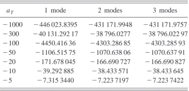
E(k). The sample results for various aT and number of modes are given in Table I.
We see that in the interesting region of not very low tem-peratures the energy converges extremely fast. In practice two modes are quite enough. The results for the Gaussian energy are plotted in Fig. 1 and will be compared with other approaches in Sec. VI. Furthermore one can show that around aT⬍⫺4.6, the Gaussian liquid energy is larger than
the Gaussian solid energy. So naturally when aT⬍⫺4.6, one
should use the Gaussian solid to set up a perturbation theory. For aT⬎⫺4.2, there is no solution for the gap equations.
C. 3D Abrikosov vortex lattice
In 3D, we expand in bases of plane waves in the third direction times previously used quasimomentum function,
共x,z兲⫽v共x兲⫹
冑
12共2兲3/2
冕
k,kzexp
冋
⫺ik 2册
⫻k共x兲exp i共kz•z兲共Ok⫹iAk兲. 共34兲The quadratic form is
K⫽ 1 8
冑
2冕
kOkGOO⫺1共k兲O⫺k⫹AkGAA⫺1共k兲A⫺k, 共35兲
where integration over k is understood as integration over Brillouin zone and over kz. Most of the derivation and
im-portant observations are intact. The modifications are
TABLE I. Mode expansion 2D.
aT 1 mode 2 modes 3 modes
⫺1000 ⫺446 023.8395 ⫺431 171.9948 ⫺431 171.9757 ⫺300 ⫺40 131.292 17 ⫺38 796.0277 ⫺38 796.022 97 ⫺100 ⫺4450.416 36 ⫺4303.286 85 ⫺4303.285 93 ⫺50 ⫺1106.515 75 ⫺1070.638 06 ⫺1070.637 91 ⫺20 ⫺171.678 045 ⫺166.690 727 ⫺166.690 827 ⫺10 ⫺39.292 885 ⫺38.433 571 ⫺38.433 645 ⫺5 ⫺7.315 3440 ⫺7.223 7197 ⫺7.223 7422
GOO⫺1共k兲⫽ kz 2 2 ⫹EO共k兲, GAA⫺1共k兲⫽ kz 2 2 ⫹EA共k兲.
The corresponding Gaussian free energy density共after in-tegration over kz兲 is f⫽v2aT⫹ A 2 v 4⫹ f 1⫹ f2⫹ f3, 共36兲 f1⫽
具
冑
EO共k兲⫹冑
EA共k兲典
k, f2⫽aT冓
1冑
EO共k兲 ⫹ 1冑
EA共k兲冔
k ⫹冓
v2冋
共2k⫹兩␥k兩兲 ⫻冑
1 EO共k兲⫹共2k⫺兩␥k冊
1冑
EA共k兲册
k , 共37兲 f3⫽冓
k⫺l冋
1冑
EO共k兲 ⫹ 1冑
EA共k兲册冋
1冑
EO共l兲 ⫹ 1冑
EA共l兲册
冔
k,l ⫹21 A冋
冓
兩␥k兩冉
1冑
EO共k兲⫺ 1冑
EA共k兲冊
冔
k册
2 .Minimizing the above energy, gap equations similar to that in 2D can be obtained. One finds that
EO共k兲⫽E共k兲⫹⌬兩␥k兩,
EA共k兲⫽E共k兲⫺⌬兩␥k兩.
E(k) can be solved by modes expansion 2D. We minimized numerically the Gaussian energy by varying v,⌬ and first
few modes of E(k). The sample results of free energy den-sity for various aT with three modes are given in Table II.
In practice two modes are also quite enough in 3D. As in the case of 2D, one can show that around aT⬍⫺5.5, the gaussian liquid energy is larger than the Gaussian solid en-ergy. So naturally when aT⬍⫺5.5, one should use the
Gaussian solid to set up a perturbation theory in 3D. When around aT⬎⫺5, there is no solution for the gap equations.
V. CORRECTIONS TO THE GAUSSIAN APPROXIMATION In this section, we calculate the lowest order correction to the Gaussian approximation 共that will be called post-Gaussian correction兲, which will determine the precision of
the Gaussian approximation. This is necessary in order to fit experiments and compare with low temperature perturbation theory and other nonperturbative methods.
First we review a general idea behind calculating system-atic corrections to the Gaussian approximation.25The proce-dure is rather similar to calculating corrections to the Hartree–Fock approximations used in fermionic systems. Gaussian variational principle provided us with the best共in a certain sense兲 quadratic part of the free energy K from which the ‘‘steepest descent’’ corrections can be calculated. The free energy is divided into the quadratic part and a ‘‘small’’ perturbation V˜ . For a general scalar theory defined in Eq. 共20兲 it takes the form
f⫽K⫹␣V˜ , K⫽12 aG⫺1abb, 共38兲 V ˜⫽⫺1 2 aD⫺1a⫹V共a兲⫺1 2 aG⫺1abb.
Here the auxiliary parameter ␣ was introduced to set up a perturbation theory. It will be set to one at the end of the calculation. Expanding the logarithm of the statistical sum in powers of␣, Z⫽
冕
Daexp共⫺K兲exp共⫺␣V˜兲 ⫽冕
Da兺
n⫽0 1 n!共␣V˜兲 nexp共⫺K兲, 共39兲one retains only the first few terms. It was shown in Ref. 26 that generally only two-particle irreducible diagrams contrib-ute to the post-Gaussian correction. The Gaussian approxi-mation corresponds to retaining only the first two terms, n ⫽0,1, while the post-Gaussian correction retains in addition the contribution of order ␣2.
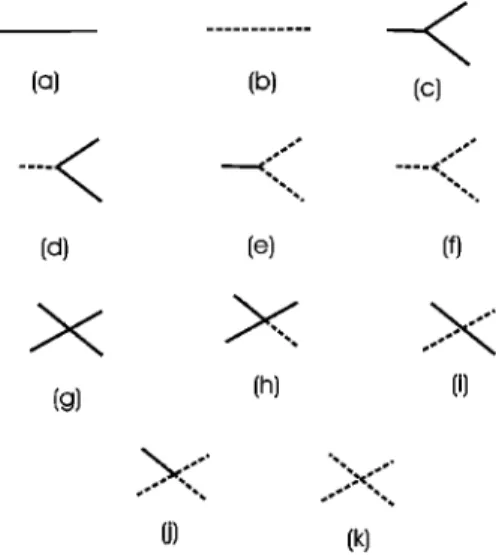
Feynman rules in our case are shown in Fig. 5. We have two propagators for fields A and O and three and four leg vertices. Using these rules the postgaussian correction is pre-sented on Fig. 6 as a set of two and three loop diagrams. The corresponding expressions are given in Appendix B. The Brillouin zone averages were computed numerically using the three modes gaussian solution of the previous section. Now we turn to discussion of the results.
TABLE II. Mode expansion 3D.
aT ⫺300 ⫺100 ⫺50 ⫺30 ⫺20 ⫺10 ⫺5.5
VI. RESULTS, COMPARISON WITH OTHER APPROACHES AND CONCLUSION
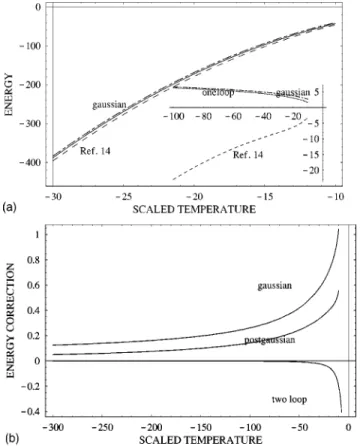
Results for LLL scaled energy, magnetization and specific heat in 2D are presented in Figs. 1, 2, and 3, respectively.
A. Energy
The Gaussian energy provides a rigorous upper bound on free energy.25Figure 1共a兲 shows the 2D Gaussian energy 共the dashed–dotted line兲, which in the range of aT from⫺30 to
⫺10 is just above the mean field 共the solid gray line兲. This is because it correctly accounts for the 共positive兲 logarithmic one loop correction of Eq.共17兲. In contrast the results of the theory by Tesanovic et al.14共the dashed gray line兲 are lower than the mean field. This reflects the fact that although the correct large 兩aT兩 limit is built in, the expansion of the
ex-pression Eq. 共19兲 gives negative coefficient of the log兩aT兩
term. This is inconsistent with both the low temperature per-turbation theory and the Gaussian approximation. The differ-ence between this theory and our result is smaller than 2% only when aT⬍30 or at small aTbelow the 2D melting line
共which occurs at aT⫽⫺13 according to Monte Carlo19 and
phenomenological estimates18,1兲 where the lines become closer again. It never gets larger than 10% though. To effec-tively quantitaeffec-tively study the model one has to subtract the dominant mean field contribution. This is done in the inset of Fig. 1共a兲. We plot the gaussian result 共the dashed–dotted line兲, the one loop perturbative result 共the solid line兲 and Eq. 共19兲 共the dashed gray line兲 in an expanded region ⫺100 ⬍aT⬍⫺10. The Gaussian approximation is a bit higher than
the one loop.
To determine the precision of the Gaussian approximation and compare with the perturbative two loop result, we fur-ther subtracted the one loop contribution on Fig. 1共b兲. As expected the post-Gaussian result is lower than the Gaussian though higher than the two loop. The difference between the Gaussian and the post-Gaussian approximation in the region shown is about兩⌬ f兩⫽0.2, which translates into 0.2% at aT
⫽⫺30, 0.4% at aT⫽⫺20 and 2% at aT⫽⫺12. The fit for
FIG. 1. Scaled free energy of vortex solid. From top to bottom, Gaussian approximation 共dashed–dotted line兲, mean field 共solid line兲, theory Ref. 14 共dashed line兲. Inset, corrections to mean field calculated using 共from top to bottom兲 Gaussian 共dashed–dotted line兲, one loop perturbation theory 共dotted line兲, and theory Ref. 14
共dashed line兲. 共b兲 More refined comparison of different
approxima-tions to free energy. Mean field as well as the one loop perturbative contributions are subtracted.
FIG. 2. Thermal fluctuations correction to magnetization of vor-tex solid. From top to bottom, one and two loop perturbation theory
共solid lines p1 and p2, respectively兲, Gaussian and post-Gaussian
approximations共dashed–dotted lines g and pg, respectively兲, theory Ref. 14共dashed line, t兲.
FIG. 3. Scaled specific heat Eq. 共45兲 normalized by the mean field. One and two loop perturbation theory共solid lines p1 and p2, respectively兲, Gaussian and post-Gaussian approximations
共dashed–dotted lines g and pg, respectively兲, theory Ref. 14 共dashed line, t兲.
the Gauss and post-Gaussian energy in the region ⫺30⬍aT ⬍⫺6 are fg2D⫽⫺ aT2 2A ⫹2 log兩aT兩⫹0.119⫺ 19.104 aT ⫺60.527 log兩aT兩 aT2 ⫹ 36.511 aT2 ⫹cv, fpg2D⫽⫺ aT 2 2A ⫹2 log兩aT兩⫹0.068⫺ 11.68 aT ⫺60.527 log兩aT兩 aT2 ⫹ 38.705 aT2 ⫹cv. In 3D, similarly one found that
fg3D⫽⫺ aT2 2A⫹2.848 35兩aT兩 1/2⫹3.1777 aT ⫺0.8137 log 2关⫺a T兴 aT . 共40兲 B. Magnetization
The dimensionless LLL magnetization is defined as
m共aT兲⫽⫺
d feff共aT兲
daT 共41兲
and the measure magnetization is
4M⫽⫺ e*h cmab
具
兩兩 2典
⫽⫺e*h cmab兩r兩 2 b⬘
2␣Tc冑 b 4, 共42兲 where is the order parameter of the original model, andr is the rescaled one, which is equal to d feff(aT)/daT. Thus4M⫽ e*h cmab b
⬘
2␣Tc冑 b 4m共aT兲. 共43兲 We plot the scaled magnetization in region ⫺30⬍aT⬍⫺6. Again, the mean field contribution dominates, so we subtract it in Fig. 2. The solid line is the one loop approximation, while the gray line is the two loop approximation. At small negative aTthe postgaussian共the upper gray dashed–dottedline兲 is very close to the two loop result, while the Gaussian approximation共the dashed–dotted line兲 is a bit lower. All of these lines are above mean field. On the other hand, the result of Ref. 14 共the gray dashed line兲 is below the mean field. Magnetization jump at the melting point is smaller than our precision of 2% at aT⫽⫺12. Our result for the Gaussian
magnetization and the post-Gaussian correction in this range can be conveniently fitted with
mg2D⫽ aT A⫺ 2 aT⫺ 19.10 aT2 ⫹ 133.55 aT3 ⫺ 121.05 log关⫺aT兴 aT3 , ⌬mpg2D⫽ 7.525 aT2 ⫺ 59.15 aT3 ⫹ 43.64 log关⫺aT兴 aT3 , respectively.
Similar discussion for the case of 3D can be deduced from Eqs. 共41兲, Eq. 共40兲, and
4M⫽⫺ e*h cmab
具
兩兩2典
⫽⫺ e*h cmab 兩r兩2 b⬘
2␣Tc冉
b 4冑
2冊
2/3 ⫽e*h cmab b⬘
2␣Tc冉
b 4冑
2冊
2/3 m共aT兲, 共44兲where the Gaussian scaled magnetization can be obtained by differentiation of Eq. 共40兲. We did not attempt to calculate the post-Gaussian correction in 3D.
C. Specific heat The scaled LLL specific heat is defined as
c共aT兲⫽⫺
d2f eff共aT兲
daT2 共45兲
and the original specific heat is related to the scaled specific heat c in 2D via C⫽ 1 42T
冋
⫺b⫹冑
ប2␣bT c 2m*b⬘
T ⫺3t⫺1⫹b 2 m共aT兲 ⫹ប 2␣T c m*b⬘
T 共⫺t⫺1⫹b兲 2 2c共a T兲册
.We plot the scaled specific heat divided by the mean field value cm f⫽1/A in the range⫺30⬍aT⬍⫺6 on Fig. 3. The
solid line is one loop approximation, while the gray line is the two loop approximation. At large兩aT兩 the post-Gaussian
共gray dashed–dotted line兲 is very closed to the one loop re-sult. Finally the Gaussian approximation 共dashed–dotted line兲 is a bit lower. All these lines are slightly above mean field. On the contrary, the result of Ref. 14共dashed gray line兲 is below the mean field. Our Gaussian result and its correc-tion in this range can be conveniently fitted with
cg cm f ⫽1⫹A
冉
2 aT2⫹ 38.2 aT3 ⫺ 521.7 aT4 ⫹ 363.2 ln关⫺aT兴 aT4冊
⌬cg cm f ⫽A冉
⫺ 15.05 aT3 ⫹ 221.1 aT4 ⫺ 130.9 ln关⫺aT兴 aT4冊
. Qualitatively the Gaussian specific heat is consistent with experiments4 which show that the specific heat first raise before dropping sharply beyond the melting point.D. Conclusions
In this paper, we applied the Gaussian variational prin-ciple to the problem of thermal fluctuations in vortex lattice state. Then the correction to it was calculated perturbatively. This generalizes corresponding treatment of fluctuations in the homogeneous phase 共vortex liquid兲 by Thouless and co-workers.5 Also Umklapp processes were included in the low temperature two loop perturbation theory expression. The results of Gaussian perturbative and some nonperturba-tive approaches were compared. The perturbanonperturba-tive corrections 共up to two loop兲 already show that the expression of the theory of Ref. 14 with the mean field subtracted has wrong sign. The Gaussian approximation provides a rigorous lower bound and is superior over the one loop result. It is valid even in the region in which the one loop diverges. In particu-lar the end of point below which the overheated solid exists as a metastable state is estimated at aT⫽⫺4.6. Similarly the
corrected Gaussian approximation is an improvement over the two loop result in the temperature range near the melting line. The calculation of the post-Gaussian correction allows us to estimate the precision, for example, the specific heat precision is higher than 1% for⫺20⬍aT⬍⫺6 共the melting
line is located at aT⫽⫺12) and higher than 0.1% for aT
⬍⫺20. The specific heat of the vortex solid is predicted to be monotonic 共unlike the theory of Ref. 14 where there is a minimum followed by a maximum兲 consistent with several experiments.4 We hope that increased sensitivity of both magnetization and specific heat experiments will test the pre-cision of the theory共see Fig. 3兲.
ACKNOWLEDGMENTS
We are grateful to our colleagues A. Knigavko, T. K. Lee, B. Ya. Shapiro, and Y. Yeshurun for numerous discussions and encouragement. The work was supported by NSC of Taiwan grant NSC#90-2112-M-009-039.
APPENDIX A
In this Appendix the basic definitions are collected. Bril-louin zone averages of products of four quasimomentum functions are defined by
k⫽
具
兩兩2kជkជ*典
,␥k⫽
具
共*兲2
⫺kជkជ
典
, 共A1兲␥k,l⫽
具
k*⫺k* ⫺ lជlជ典
.We also need a more general product
具
k1
*k2k*3k4
典
inor-der to calculate post-Gaussian corrections. This is just a per-turbative four-leg vertex,
具
k*1k2*k3k4典
⫽exp冋
i2 2 共n1 2⫺n 1兲⫹i 2 a⌬n1k3y册
␦ q关k 1⫺k2 ⫹k3⫺k4兴关k1⫺k2,k2⫺k4兴, 共A2兲 关l1,l2兴⫽兺
Q exp冋
⫺兩l1⫹Q兩 2 2 ⫹i共l1x⫹l2x兲Qy⫺i共l1y ⫹l2y兲Qx册
exp关i共l1x⫹l2x兲l1y兴,where Q are reciprocal lattice vectors,
Q⫽m1˜d1⫹m2d˜2. 共A3兲 Here k1⫺k2⫹k3⫺k4⫽n1d˜1⫹n2d˜2is assumed and the basis of reciprocal lattice is ˜d1⫽(2/a⌬)关1,⫺(1/
冑
3)兴, d˜2 ⫽关0,(4/a⌬冑
3)兴, a⌬⫽冑
4/冑
3 . It is dual to the latticee1⫽(a⌬,0), d2⫽关(a⌬/2),(a⌬
冑
3/2)兴. When k1⫺k2⫹k3 ⫺k4⫽n1d˜1⫹n2˜d2 the quantity vanishes. The delta function differs from the Kroneker,␦q关k兴⫽
兺
Q ␦关k⫹Q兴.
From the above formula, one gets the following expansion of k: k⫽
兺
m1,m2 exp冋
⫺兩X兩 2 2 ⫹ik•X册
⫽兺
n exp冋
⫺ a⌬2 2 n册
n共k兲, 共A4兲 where X⫽n1d1⫹n2d2.To simplify the minimization equations we used the fol-lowing general identity. Any sixfold (D6) symmetric func-tion F(k) 关namely a function satisfying F(k)⫽F(k
⬘
), where k,k⬘
is related by a 2/6 rotation兴 obeys冕
kF共k兲␥k␥k,l⫽
␥l
A
冕
kF共k兲兩␥k兩2, 共A5兲
where␥k and␥k,lare defined in Eq.共A1兲. This can be seen
by expanding F in Fourier modes and symmetrizing.
FIG. 4. Reciprical hexagonal lattice points X belonging to three lowest order ‘‘stars’’ in the mode expansion ofk.
APPENDIX B
In this Appendix we specify Feynman rules and collect expressions for diagrams. The solid line Fig. 5共a兲 represents O and the dashed line Fig. 5共b兲 represents A. Figure. 5共c兲 is a vertex with three O. In the coordinate space, it is 2v关O(O⫹)2⫹c.c.兴. Figure 5共c兲 is ⫺2iv⫹O2A⫹ ⫺4ivOO⫹A⫹⫹c.c, Fig. 5共g兲 is 1
2兩O(x)兩
4, Fig. 5共h兲 is 2OO⫹(AO⫹⫺OA⫹), and Fig. 5共i兲 is 4OO⫹AA⫹ ⫺关O2(A⫹)2⫹c.c.兴.
Other vertices, for example, formulas for diagrams in Fig. 5共e兲, 5共f兲, 5共j兲, and 5共k兲, can be obtained by substituting O→iA,A→⫺iO from formulas for diagrams in Fig. 5共d兲, 5共c兲, 5共h兲, and 5共g兲, respectively.
The propagator in coordinate space can be written as
具
O⫹共x兲O⫹共y兲典
⫽4冕
k EO共k兲k*共x兲⫺k* 共y兲⫽4PO⫹共x,y兲,具
O共x兲O共y兲典
⫽4冕
k EO共k兲k共x兲⫺k共y兲⫽4PO⫺共x,y兲, 共B1兲具
O共x兲O⫹共y兲典
⫽4冕
k EO共k兲k共x兲k*共y兲⫽4PO共x,y兲. Functions PA⫹(x, y ), PA⫺(x, y ), PA(x, y ) can be definedsimi-larly.
One finds three loops contribution to free energy from two OOOO vertex contraction, see Fig. 6共a兲, ⫺1/16(2)5兰 x
具
foooo典
y, foooo⫽4具
兩PO兩4⫹兩PO⫹兩 4⫹4兩P OPO⫹兩 2典
y. 共B2兲Coordinates are not written explicitly since all of them are the same PO(x,y ), etc.
The contribution from the diagrams in Fig. 6共b兲 is ⫺1/16(2)5兰x
具
foooa典
y, and foooa⫽兩PO兩2共⫺16PO⫹P⫺A⫹8POPA*兲⫹兩PO⫹兩2共⫺8P O ⫹P A ⫺ ⫹16POPA*兲⫹c.c. 共B3兲The diagrams in Fig. 6共c兲 are ⫺1/16(2)5兰x
具
fooaa典
yandfooaa⫽16共兩PO兩2⫹兩PO⫹兩2兲共兩PA兩2⫹兩PA⫹兩2兲⫹4共关PO⫹兴2关PA⫺兴2 ⫹PO 2关P A 2兴 *⫹c.c.兲⫺32共PO⫺PO*PA⫹PA⫹c.c.兲. 共B4兲
The diagrams in Fig. 6共f兲 are ⫺v2/16(2)4兰x
具
fooo典
yandfooo⫽兩PO兩2共16PO⫹共x兲共y兲⫹8PO*共x兲*共y兲⫹c.c.兲
⫹兩PO⫹兩 2共8P O ⫹共x兲共y兲⫹16P O *共x兲*共y兲⫹c.c.兲. 共B5兲 The diagrams in Fig. 6共h兲 are ⫺v2/16(2)4兰x
具
fooa典
yandfooa⫽⫺8共PO⫺兲 2P A ⫹*共x兲*共y兲⫺16共兩P O兩2⫹兩PO⫹兩 2兲 ⫻„PA⫹共x兲共y兲⫺PA*共x兲共y兲… ⫹8PO 2 PA**共x兲共y兲⫺32POPO⫺关PA⫹*共x兲共y兲 ⫺PA**共x兲*共y兲兴⫹c.c. 共B6兲
Other contributions, Fig. 6共e兲, 6共d兲, 6共i兲, 6共g兲 can be obtained by substituting PO↔PA, PA⫹↔⫺PO,⫹ PA⫺↔⫺PO⫺ in Eq.
共B2兲, Eq. 共B3兲, Eq. 共B5兲, and Eq. 共B6兲.
FIG. 5. Feynman rules of the low temperature perturbation theory. The solid line共a兲 denoted the O mode propagator, while the dashed line 共b兲 denotes the A mode propagator. Various three leg and four leg vertices are presented in 共c兲–共f兲 and 共g兲–共k兲, respectively.
FIG. 6. Contributions to the post-Gaussian correction to free energy.
*Electronic mail: [email protected]
†Electronic mail: [email protected]
1G. Blatter, M.V. Feigel’man, V.B. Geshkenbein, A.I. Larkin,
and V.M. Vinokur, Rev. Mod. Phys. 66, 1125共1994兲.
2D.R. Nelson, Phys. Rev. Lett. 60, 1973共1988兲.
3E. Zeldov, D. Majer, M. Konczykowski, V.B. Geshkenbein, V.M.
Vinokur, and H. Shtrikman, Nature共London兲 375, 373 共1995兲.
4M. Roulin, A. Junod, A. Erb, and E. Walker, J. Low Temp. Phys. 105, 1099共1996兲; A. Schilling et al., Phys. Rev. Lett. 78, 4833 共1997兲; S.W. Pierson and O.T. Valls, Phys. Rev. B 57, R8143 共1998兲.
5D.J. Thouless, Phys. Rev. Lett. 34, 946共1975兲; G.J. Ruggeri and
D.J. Thouless, J. Phys. F: Met. Phys. 6, 2063共1976兲.
6G.J. Ruggeri, Phys. Rev. B 20, 3626共1979兲.
7T. Barnes and G.I. Ghandour, Phys. Rev. D 22, 924共1980兲; A.
Kovner and B. Rosenstein, ibid. 39, 2332 共1989兲; 40, 504
共1989兲. 8
N.K. Wilkin and M.A. Moore, Phys. Rev. B 47, 957共1993兲.
9D. Li and B. Rosenstein, Phys. Rev. Lett. 86, 3618共2001兲. 10D. Li and B. Rosenstein, preceding paper, Phys Rev. B 65,
024513共2001兲.
11B. Rosenstein, Phys. Rev. B 60, 4268共1999兲.
12H.C. Kao, B. Rosenstein, and J.C. Lee, Phys. Rev. B 61, 12 352 共2000兲. Note that in this reference the one loop coefficient is
missing.
13One might object on the basis of Mermin–Wagner theorem, N.D.
Mermin and H. Wagner, Phys. Rev. Lett. 17, 1133共1966兲, that in 2D the gauge U共1兲 and translation symmetry cannot be broken spontaneously. We address this concern below. The situation is similar to the one encountered while directly expanding energy in 1/aT recently performed by one of us to the two loop order.
Although the vortex solid state has only a quasi-long-range
or-der rather than infinite-long-range oror-der, in certain sense the state is much closer to the Gaussian solid state defined in this paper than to the Gaussian liquid state used in the high tempera-ture perturbative expansion.
14Z. Tesanovic and A.V. Andreev, Phys. Rev. B 49, 4064共1994兲; Z.
Tesanovic, L. Xing, L. Bulaevskii, Q. Li, and M. Suenaga, Phys. Rev. Lett. 69, 3563共1992兲.
15D. Li and B. Rosenstein, Phys. Rev. B 60, 9704共1999兲. 16D. Li and B. Rosenstein, Phys. Rev. B 60, 10 460共1999兲. 17
D.J. Thouless, Phys. Rev. Lett. 34, 946共1975兲; A.J. Bray, Phys. Rev. B 9, 4752共1974兲.
18S. Hikami, A. Fujita, and A.I. Larkin, Phys. Rev. B 44, R10 400 共1991兲; E. Brezin, A. Fujita, and S. Hikami, Phys. Rev. Lett. 65,
1949共1990兲; 65, 2921 共1990兲.
19Y. Kato and N. Nagaosa, Phys. Rev. B 48, 7383共1993兲; J. Hu and
A.H. Macdonald, Phys. Rev. Lett. 71, 432共1993兲; J.A. ONeill and M.A. Moore, Phys. Rev. B 48, 374共1993兲.
20V. Zhuravlev and T. Maniv, Phys. Rev. B 60, 4277共1999兲. 21G. Eilenberger, Phys. Rev. 164, 628共1967兲.
22K. Maki and H. Takayama, Prog. Theor. Phys. 46, 1651共1971兲. 23A. Lopatin and G. Kotliar, Phys. Rev. B 59, 3879共1999兲. 24M.A. Moore, T.J. Newman, A.J. Bray, and S.-K. Chin, Phys. Rev.
B 58, 9677共1998兲.
25H. Kleinert, Path Integrals in Quantum Mechanics, Statistics, and Polymer Physics共World Scientific, Singapore, 1995兲.
26J.M. Cornwall, R. Jackiw, and E. Tomboulis, Phys. Rev. D 10,
2428共1974兲; R. Ikeda, J. Phys. Soc. Jpn. 64, 1683 共1994兲; 64, 3925共1995兲.
27Note that similar simplification occurs in the large N approach
developed in Ref. 23. Consequently their Anzatz is in fact a rigorous solution to their gap equations.